Int. J. Industrial Mathematics Vol. 1, No. 1 (2009) 1-11
A Method to Approximate Solution of the First
Kind Abel Integral Equation Using Navot's
Quadrature and Simpson's Rule
Mohammad Ali Fariborzi Araghia, Soodabeh Yazdania
(a) Department of Mathematics, Islamic Azad University, Central Tehran Branch, P.O. Box 13185.768, Tehran, Iran.
||||||||||||||||||||||||||||||||-Abstract
In this paper, we present a method for solving the rst kind Abel integral equation. In this method, the rst kind Abel integral equation is transformed to the second kind Volterra integral equation with a continuous kernel and a smooth deriving term expressed by weakly singular integrals. By using Sidi's sinm - transformation and modied Navot-Simpson's
integration rule, an algorithm for solving this kind of integral equation is proposed, then the convergence of algorithm is derived. Some numerical results show the eciency of the mentioned method.
Keywords: The rst kind Abel integral equation, Simpson's rule, Sidi's sinm- transformation, Zeta function, Navot's quadrature.
|||||||||||||||||||||||||||||||||{
1
Introduction
The rst kind Abel integral equation Z x
0
H(x; y)
(x y)f(y)dy = g(x) (0 x 1; 0 < < 1); (1.1)
frequently appears in many physical and engineering problems, e.g., semi-conductors, scat-tering theory, seismology, heat conduction, metallurgy, uid ow, chemical reactions and population dynamics, etc.
There are many classes of numerical methods for the approximate solution of Eq. (1.1) such as product-integration methods, collocation methods, fractional multistep methods, etc.
Ya-Ping Liu and Lu Tao in [1] proposed quadrature methods and their extrapolation for solving Eq. (1.1). In [2], a method in order to solve the second kind singular Volterra integral equations by modied Navot-Simpson's quadrature rule was proposed. In this paper, we propose a similar approach for solving (1.1) based on the method presented in [1].
Since solving the rst kind Abel integral equation is an ill-posed problem we transform that into the second kind. For this purpose, in (1.1) we replace x by s, multiply both sides
by 1
(x s)1 and integrate both sides in [0; x] with respect to s then the following relation
is obtained: Z x
0
Z s
0
H(s; y)
(x s)1 (s y)f(y)dyds =
Z x
0
g(s) (x s)1 ds:
The double integral in above relation can be written as R0x(Ryx (x s)H(s;y)1 (s y)ds)f(y)dy.
Let
L(x; y) = Z x
y
H(s; y)
(x s)1 (s y)ds ; G(x) =
Z x
0
g(s) (x s)1 ds:
If we apply the change of variables s = y + (x y) for L(x; y) and s = x for G(x) then,
L(x; y) = Z 1
0
H(y + (x y); y)
(1 )1 d; (1.2)
and
G(x) = xZ 1 0
g(x)
(1 )1 d: (1.3)
Therefore, (1.1) can be written as Z x
0 L(x; y)f(y)dy = G(x): (1.4)
By dierentiating (1.4) with respect to x, we get d
dx Z x
0 L(x; y)f(y)dy = G
0(x) =) L(x; x)f(x) +Z x 0
@
@xL(x; y)f(y)dy = G0(x):
Since L(x; x) = sin()H(x;x) 6= 0 for 0 x 1 and G(0) = 0, then we can write,
f(x) + Z x
0 ~L(x; y)f(y)dy = V (x); 0 x 1; (1.5)
where ~L(x; y) = Lx(x; y)=L(x; x) and V (x) = G0(x)=L(x; x). The Eq. (1.5) is the second
kind Volterra integral equation whose kernel and deriving term are expressed by weakly singular integrals.
Since the solution f(x) of (1.5) or its derivative f0(x) may be unbounded at the origin,
Baratella and Orsi [3] proposed to take the change of variable x = (t) = tq, (0 t 1)
in (1.5), where q is an undetermined positive constant. Then (1.5) is written as
f((t)) + Z (t)
Letting y = (s), we have
f((t)) + Z t
0 ~L((t); (s))f((s))
0(s)ds = V ((t)) (0 t 1): (1.6)
Multiply (1.6) by 0(t) and set
u(t) = 0(t)f((t)); (t) = 0(t)V ((t)); L(t; s) = 0(t)~L((t); (s)):
Consequently the Eq. (1.6) is simplied as
u(t) + Z t
0 L(t; s)u(s)ds = (t); (0 t 1): (1.7)
With a suitable choice of the parameter q we can ensure that the solution u(t) and (t) of (1.7) are suciently smooth [1].
3
The numerical method
Since the kernel and the deriving term of the integral equation (1.7) are expressed by weakly singular integrals, we must use a numerical method which is able to compute these integrals with weak singularity at the end points. For this purpose, Navot's quadrature rule is used. This special quadrature is applied for functions having a singularity of any type on or near the integration interval.
We recall that, in the interval [0,1], the trapezoidal rule is dened as, T f = 1 N
PN 1
j=1 f(Nj)+ 1
2N[f(0) + f(1)]; and for the midpoint rule, Mf = N1
PN
j=1f(2j 12N ). So, if N is even then
the Simpson's integration rule can be dened as [4,5], Sf = 2
3Mf + 13T f. Now, we can
imply the following lemma in the interval [a,b] for introducing the modied Simpson's rule by Navot's Quadrature. This lemma is an improvement of the asymptotic expansion of the trapezoidal rule which has been presented in [1].
Lemma 3.1. Let g(x) 2 C2l+1[a; b](l 2 Z+), G(x) = (b x)g(x), h = (b a)=N, N is
even and xi = a + ih, i = 0; 1; : : : ; N, then the modied Simpson's integration rule SN(G)
has an asymptotic expansion as follows,
SN(G) = h3G(x0) +43h
N 2
X
i=1
G(x2i 1) +23h bN 1X2 c
i=1
G(x2i)
g(b)
2 3( ;
1 2) +
1 3( )
h1+ (2.1)
= Z b
a (b x)
g(x)dx +Xl j=1
PjG(2j 1)(a)h2j
+X2l
j=1
( 1)jg(j)(b)hj!j++1
1 3 +
2
3(2 j 1)
( j) + O(h2l+1);
where 1 < < 0, ( ;1
2) = (2 1)( ), (x) is the Riemann-Zeta function and
Proof. In [1,4] the modied trapezoidal rule Th0(G) has been introduced by using Navot's
quadrature as follows:
Th0(G) = h
0
2G(x00) + h0
M 1X
j=1
G(x0j) + ( )g(b)h01+
= Z b
a (b x)
g(x)dx +Xl j=1
B2j
(2j)!G(2j 1)(a)h02j (2.1)
+X2l
j=1
( 1)jg(j)(b)hj!0j++1( j) + O(h02l+1);
where, (x) is the Riemann-Zeta function and B2j; j = 1; :::; l, are the Bernoulli
num-bers and x0
j = a + jh0; j = 0; :::; M 1; h0 = b aM . The similar formula can be written for
the modied mid-point rule as follows [5]:
Mh0(G) = h0
M
X
j=1
G(x0j h20) (2 1)( )g(b)h01+:
Since the number of the points when we combine the modied trapezoidal and mid-point rules is N = 2M which is even, hence bN 1
2 c = N2 1 and bN2c = N2. If h = b aN
then, x2j 1 = x0j h; j = 1; 2; :::; M and x2j = x0j; j = 1; 2; :::; M 1; hence we can compute
SN(G) in the interval [a; b] as follows:
SN(G) = 23Mh0(G) +1
3Th0(G) = 2
3[h0
M
X
j=1
G(x0j h20) (2 1)( )g(b)h01+]+13[h20G(x00)+h0
M 1X
j=1
G(x0j) ( )g(b)h01+] =
h
3G(x0) + 4 3h
N 2
X
j=1
G(x2j 1) +23h
N 2 1
X
j=1
G(x2j) [23( ;12) +13( )]g(b)h1+:
Also, if Pj; j = 1; 2; :::; l; are the constant values independent of h, the following relation
can be proved similarly by using (2.1).
SN(G) =
Z b
a (b x)
g(x)dx +Xl j=1
PjG(2j 1)(a)h2j
+X2l
j=1
( 1)jg(j)(b)hj!j++1
1 3+
2
3(2 j 1)
( j) + O(h2l+1):
Since the periodization methods play an important roles in increasing accuracy of quadrature rules, we will use a Sidi's sinm- transformation [6], which is constructed by
m(y) = m(y)
m(1) with m(y) =
Z y
0 (sin(t))
mdt; m = 1; 2; : : : :
m(y) has the following asymptotic expansions
(
m(y) "mym+1+P1i=1"m;iym+1+2i as y ! 0+;
m(y) 1 ^"m(1 y)m+1 P1i=1^"m;i(1 y)m+1+2i as y ! 1 ; (2.2)
where "m6= 0, ^"m6= 0, "m;i and ^"m;i, (i = 1; 2; : : : ) are all constants.
From (1.2),
Lx(x; y) = @x@ L(x; y) =
Z 1
0 H
0(y + (x y); y) 1
(1 )1 d;
where H0(x; y) = @
@xH(x; y). By Letting = m(t), then
Lx(x; y) =
Z 1
0 (x; y; t)dt; (2.3)
with
(x; y; t) = H0(y +
m(t)(x y); y) ( m(t)) 1
(1 m(t))1 0
m(t): (2.4)
By (2.2), there are functions B(t) and C(t) such that
0 m(t)
(1 m(t))1 = (m + 1)(^"m)
(1 t)(m+1) 1 1 C(t)(1 t)2
(1 B(t)(1 t)2=(^"m))1 ;
which has a zero or pole of th order at t = 1, where = (m + 1) 1. Then, we have
(x; y; t) = (1 t)(x; y; t);
where,
(x; y; t) = (m + 1)(^"m)H0(y + m(t)(x y); y)( m(t))
1 (1 C(t)(1 t)2)
(1 B(t)(1 t)2=(^"m))1 :
We observe that is nonsingular at t = 1.
From lemma 2.1, since m(0) = 0 and m(1) = 1, we may derive an approximation
Lh
x(x; y) of Lx(x; y) as follows:
Lhx(x; y) = 43
N 2
X
j=1
h(x; y; t2j 1) +23 bN 1
2 c
X
j=1
h(x; y; t2j)
(m + 1)(^"m)h+1H0(x; y)
2 3( ;
1 2) +
1 3( )
: (2.5)
For the kernel L(x; y) of (1.7) the corresponding approximate expression is
Lh(t; s) = 0(t)Lhx((t); (s))
L((t); (t)) ; (2.6)
where L((t); (t)) = H((t);(t))sin() 6= 0. On the other hand by (1.3),
G0(x) = x 1 Z 1
0
g(x)
(1 )1 d + x
Z 1
0
g0(x)
(1 )1 d
= x 1Z 1
0 G1(x; )d + x Z 1
0 G2(x; )d;
where,
G1(x; t) = (1 g(x m(t)) m(t))1
0
m(t); G2(x; t) = g 0(x
m(t))
(1 m(t))1 m(t) 0 m(t):
In (1.7),
(t) = L((t); (t))0(t)G0((t)) = L((t); (t))0(t)((t)) 1 Z 1
0 G1((t); )d +
0(t)((t))
L((t); (t)) Z 1
0 G2((t); )d:
We put
I1(t) =
0(t)((t)) 1
L((t); (t)) Z 1
0 G1((t); )d;
and
I2(t) =
0(t)((t))
L((t); (t)) Z 1
0 G2((t); )d:
We have G0(x) = O(x 1), as x ! 0, and since (t) = tq we have that I 1(t) =
O(tq 1) and I2(t) = O(tq+q 1), as t ! 0. Choosing q > 1
, we get I1(0) = I2(0) = 0.
Similar to above discussion, we can obtain approximate expressions for I1(t) and I2(t) as
follows:
I1h(t) = L((t); (t))0(t)((t)) 1 2 44 3 N 2 X j=1
hG1((t); t2j 1) +23 bN 1
2 c
X
j=1
hG1((t); t2j)
(m + 1)h+1(^"m)g((t))
2 3( ;
1 2) +
1 3( )
(0 t 1); (2.7)
and
I2h(t) = L((t); (t))0(t)((t)) 2 44 3 N 2 X j=1
hG2((t); t2j 1) +23 bN 1
2 c
X
j=1
hG2((t); t2j)
(m + 1)h+1(^"m)g0((t))
2 3( ;
1 2) +
1 3( )
Then, the approximation of (t) is
h(t) = I1h(t) + I2h(t): (2.9)
By (2.6) and (2.9), the following approximate integral equation is derived:
u(t) + Z t
0 L
h(t; s)u(s)ds = h(t): (2.10)
Now, we can apply the Simpson's rule to derive the numerical solution of (2.10).
Algorithm (Simpson's rule) (
us
0= s(t0) = 0
us
i = h(ti) h3Pij=0wijLh(ti; tj)usj; i = 1; : : : ; N (2.11)
where, wi0 = wii = 1, wij = 4 (j = 2k 1), wij = 2(j = 2k), k 1; 0 < j < i,
i = 0; 1; : : : ; N.
By this algorithm, fus
ig, i = 0; : : : ; N are found and fusi=0(ti)g will be the approximate
of the solution ff((ti))g of (1.7).
4
Convergence and error estimate
Assume that the data function is not perturbed by noise, then approximations Lh(t; s)
and h(t) satisfy the following lemma.
Lemma 4.1. Let H(x; :), g(x) 2 C6[0; 1], then the errors Lh(t; s) L(t; s) and h(t) (t)
have the estimates
Lh(t; s) L(t; s) = O(h); (3.1)
and
h(t) (t) = O(h); (3.2)
where = minf + 3; 4g.
Proof. Since H(x; :); g(x) 2 C6[0; 1], it follows that (:; :; t), 2 C5[0; 1]. By lemma 2.1 with
l = 2,
~Lh(x; y) =Z 1 0 (1 t)
(x; y; t)
L(x; x) dt +
2
X
j=1
Pj
(2j 1)(x; y; 0)
L(x; x) h2j
+X4
j=1
( 1)j(j)(x; y; 1)hj++1
L(x; x)j!
1 3 +
2
3(2 j 1)
( j) + O(h5):
Then we have,
~Lh(x; y) ~L(x; y) = T
with
T1= P1
(1)(x; y; 0)
L(x; x) ;
T2= P2
(3)(x; y; 0)
L(x; x) ;
T3=
(1)(x; y; 1)
L(x; x)
1 3 +
2
3(2 1 1)
( 1);
T4=
(2)(x; y; 1)
2L(x; x)
1 3+
2
3(2 2 1)
( 2);
T5=
(3)(x; y; 1)
6L(x; x)
1 3 +
2
3(2 3 1)
( 3);
T6=
(4)(x; y; 1)
4!L(x; x)
1 3+
2
3(2 4 1)
( 4):
By letting
R(t) = (1 B(t)(1 t)1 C(t)(1 t)2=(^" 2
m))1 ;
then, @
@t(x; y; t) = (m + 1)(^"m)(H(2)(y + m(t)(x y); y)
(x y) 0m(t)R(t)( m(t))1 + H0(y + m(t)(x y); y)( m(t))1 R0(t)
+ H0(y +
m(t)(x y); y)R(t)( m(t)) m0 (t)):
Since 0
m(1) = 0, R0(1) = 0, m(0) = 0, m0 (0) = 0 we get @t@(x; y; 1) = 0 and @
@t(x; y; 0) = 0. Therefore, T1(x; y) = 0, and T3(x; y) = 0. From L(t; s) = 0(t)~L((t); (s)),
(3.1) is proved.
Using the same technique we can also prove (3.2). This completes the proof of lemma 3.1.
In order to obtain an error estimate of algorithm, we need the following discrete Gron-wall inequality.
Lemma 4.2. [1].If a nonnegative sequence fyn; n = 0; : : : ; Ng satises y0 = 0, yn
A + BhPn 1j=0yj, 1 n N, h = N1, then
max
0iNyi Ae B
where A and B are positive constants independent of h. The error of algorithm is estimated as follows.
Theorem 4.3. Assume that H(x; :); g(x) 2 C6[0; 1], H(:; y) 2 C5[0; 1] and the step size h
is suciently small, then the error es
i = u(ti) usi, i = 0; 1; : : : ; N of the above Algorithm
is obtained by
max
1iNje s
Proof. By Euler-Maclaurian formula of the Simpson's integration rule, (1.7) becomes the following equality,
(
(t0) = u(t0) = 0
(ti) = u(ti) +h3 Pij=0wijL(ti; tj)u(tj) + Q1(ti)h4+ O(h5); i = 1; 2; : : : ; N;
with
wi0= wii= 1; wij = 2 (j = 2k); wij = 4 (j = 2k 1); k 1;
and,
Q1(ti) = c d 3
ds3(L(ti; s)u(s))s=ts=0i; c = 1801
By lemma 3.2 we have,
h(t
i) = (ti) + O(h)
= u(ti) +h3 i
X
j=0
wijLh(ti; tj)u(tj) + Q1(ti)h4+ O(h5) + O(h); (3.4)
where, = minf + 3; 4g.
Subtracting (3.4) from (2.11), we get (
es 0= 0
es i = h3
Pi
j=0wijLh(ti; tj)esj+ Ei;t(ti; t; u(t));
where, Ei;t(ti; t; u(t)) = Q1(ti)h4+ O(h). Let
A = max
1iN0t1max jEi;t(ti; t; u(t))j;
since 1 < < m, we can derive A = O(h) where 2 < 4.
Now let
B = sup
h>01iNmax 0jimax jL h(t
i; tj)j;
then we have
jesij h3B
i
X
j=0
jesij + A
By lemma 3.3, there is a constant dM independent of h satisfying
max
1iNje s
ij AeB dMh; 2 < 4:
This completes the proof.
5
Numerical examples
In this section, we apply the above algorithm to solve the following examples [1]. We use m = 2 or let = 2(t) = (21 ) (2t sin 2t). The programs have been provided with
Example 5.1. In this example, The integral equation (1.1) is considered with
= 12; H(x; y) = x2y + e; g(x) = 3x4 + 4ex:
The exact solution of the integral equation is f(x) = 8px. We use a smoothing transfor-mation x = (t) = t2. The relative errors are shown in Table 1.
Table 1. The errors of the example 1 at x = 1:0 N Numerical solution error
2 8.7770128 9.71266E-2
4 8.6105208 7.63151E-2
8 8.3686739 4.60842E-2
16 8.03111328 3.88916E-3
32 8.01611856 2.01482E-3
64 8.000245921 3.07401E-5
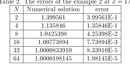
Example 5.2. In this example, we consider the integral equation 1
(1=2) Z x
0
1
(x y)1=2f(y)dy =
p
: (0 x 1)
The exact solution is f(x) = p1
x. Since the solution is unbounded at the origin. We
applying a smoothing transformation x = (t) = t4. Then, the relative errors are shown
in Table 2.
Table 2. The errors of the example 2 at x = 1:0 N Numerical solution error
2 1.399561 3.99561E-1
4 1.135846 1.35846E-1
8 1.0425398 4.25398E-2
16 1.00773894 7.73894E-3
32 1.0000833910 8.33910E-5 64 1.0000198145 1.98145E-5
6 Conclusions
Many of important mechanical and physical problems are converted to a type of the rst kind Abel integral equations. In this work, for solving these kinds of integral equations, we presented a numerical method to approximate the solution by using Navot's quadrature and Simpson's rule. We apply the integral equation which has a singularity at one of the endpoints. One can improve this technique to use the Navot's quadrature and modify it for the case that there are singularity at both of the endpoints of the integration interval.
References
[2] M. A. Fariborzi Araghi, H. D. Kasmaei, Numerical Solution of the second kind singu-lar Volterra integral equations by modied Navot-Simpson's quadrature, Int. J. open problems Compt. math., Vol. 1, No. 2, Dec. 2008, 201-213.
[3] P. Baratella, A. P. Orsi. A new approach to the numerical solution of weakly singular Volterra integral equations. J. Comp. Appl. Math. 163(2004) 401-418.
[4] J. Navot, A further extension of Euler-Maclaurin summation formula. J. Math. Phys. 41(1962) 155-184.
[5] J. N. Lyness, B. W. Ninham, Numerical quadrature and asymptotic expansions. Math. comp. 21(1967) 162-178.