Unsupervised Learning of Latent Structure from Linear and Nonlinear Measurements

(1)

Unsupervised Learning of Latent Structure from Linear and

Nonlinear Measurements

A DISSERTATION

SUBMITTED TO THE FACULTY OF THE GRADUATE SCHOOL OF THE UNIVERSITY OF MINNESOTA

BY

Bo Yang

IN PARTIAL FULFILLMENT OF THE REQUIREMENTS FOR THE DEGREE OF

DOCTOR OF PHILOSOPHY

Nicholas D. Sidiropoulos, Advisor

(2)

c

(3)

Acknowledgments

My sincerest gratitude goes to my advisor, Prof. Nikos Sidiropoulos. He helped me navigate through the mist at the frontier of human knowledge with his technical acumen. He taught me, directly and indirectly, many invaluable lessons on the various aspects of conducting research: formulating problems, solving problems, and presenting results. He clearly identified my weaknesses and suggested ways to overcome them. In a way, he practices the ancient wisdom of Confucius, “to teach in accordance with their aptitude”, and I have benefited greatly.

I am deeply indebted to Dr. Xiao Fu. Dr. Fu was a postdoctoral researcher with our research group when I joined the group. Effectively, he served as my first-order advisor. My collaboration with him put me in a unique position to capitalize on his outstanding technical capability, as well as his very good taste in research. He taught me the importance of focusing on real research problems – problems that have a clear motivation and significance.

I am very grateful to Professor Georgios Giannakis, Professor George Karypis, Professor Mingyi Hong for serving on my thesis committee. They have influenced me greatly, through lectures, personal interactions, as well as their research products (papers, books, and software codes). Their commitment to excellence in research and teaching sets good examples for me to follow. I would also like to thank several other faculty members in University of Minnesota that have helped me vastly through their wonderful lectures: Professor Zhi-Quan Luo, Professor Yousef Saad, Professor Arindam Banerjee, and Professor Jarvis Haupt.

(4)

current lab-mates: Balasubramanian Gopalakrishnan, John Tranter, Cheng Qian, Kejun Huang, Aritra Konar, Mikael Sorensen, Charilaos Kanatsoulis, Ahmed Zamzam, Nikos Kargas, Faisal Almutairi, Mohamed Salah Ibrahim, and Magda Amiridi. I am also very thankful to my friends Yanning Shen, Gang Wang, Liang Zhang, Tianyi Chen, Zhimeng Yin, Shuai Wang, and many others.

Finally, I want to thank my family: my mother Guixian Li, my late father Jianbin Yang, my sister Ling Yang, my wife Xi Chen and my son Bi-Qiang Will Yang. This work could not have been done without their unconditional love and support.

(5)

Dedication

To my family.

(6)

Abstract

The past few decades have seen a rapid expansion of our digital world. While early dwellers of the Internet exchanged simple text messages via email, modern citizens of the digital world conduct a much richer set of activities online: entertainment, banking, booking for restaurants and hotels, just to name a few. In our digitally enriched lives, we not only enjoy great convenience and efficiency, but also leave behind massive amounts of data that offer ample opportunities for improving these digital services, and creating new ones. Meanwhile, technical advancements have facilitated the emergence of new sensors and networks, that can measure, exchange and log data about real world events. These technologies have been applied to many different scenarios, including environmental monitoring, advanced manufacturing, healthcare, and scientific research in physics, chemistry, bio-technology and social science, to name a few. Leveraging the abundant data, learning-based and data-driven methods have become a dominating paradigm across different areas, with data analytics driving many of the recent developments.

However, the massive amount of data also bring considerable challenges for analytics. Among them, the collected data are often high-dimensional, with the true knowledge and signal of interest hidden underneath. It is of great importance to reduce data dimension, and transform

the data into theright space. In some cases, the data are generated from certain generative

models that areidentifiable, making it possible to reduce the data back to the original space. In

addition, we are often interested in performing some analysis on the data after dimensionality reduction (DR), and it would be helpful to be mindful about these subsequent analysis steps when performing DR, as latent structures can serve as a valuable prior. Based on this reasoning, we develop two methods, one for the linear generative model case, and the other one for the nonlinear case. In a related setting, we study parameter estimation under unknown nonlinear distortion. In this case, the unknown nonlinearity in measurements poses a severe challenge. In practice, various mechanisms can introduce nonlinearity in the measured data. To combat this challenge, we put forth a nonlinear mixture model, which is well-grounded in real world applications. We show that this model is in fact identifiable up to some trivial indeterminancy. We develop an efficient algorithm to recover latent parameters of this model, and confirm the effectiveness of our theory and algorithm via numerical experiments.

(7)

List of Tables

2.1 Comparison of cosine distance in data and latent domain. Data samples are taken

from two clusters for each dataset. . . 7

2.2 Clustering and factorization accuracy for identifiable NMF vs. SNR2, forI = 50, J = 1000, F = 7, K = 10, SNR1 = 15dB. . . 30

2.3 Clustering and factorization accuracy for identifiable NMF vs. SNR1, forI = 50, J = 1000, F = 7, K = 10, SNR2 = 10dB. . . 30

2.4 Simulation comparison of the clustering methods, identifiable NMF model. I = 50,F = 7,J = 100K. . . 32

2.5 Clustering and factorization accuracy for identifiable VolMin vs. SNR2, for I = 50, J = 1000, F = 7, K = 10. . . 34

2.6 MSE and clustering accuracy of JTKM vs. NTF for variousF =K. . . 35

2.7 Simulation comparison of proposed JNKS with LS3C . . . 36

2.8 The Legal cluster identified by the three methods, Bold entries are miss-clustered. 40 3.1 Evaluation on the RCV1-v2 dataset . . . 58

3.2 Evaluation on the 20Newsgroup dataset. . . 59

3.3 Evaluation on the raw MNIST dataset. . . 61

3.4 Evaluation on pre-processed MNIST . . . 62

3.5 Evaluation on the Pendigits dataset . . . 66

(12)

List of Figures

2.1 The effect of distance distortion introduced byW. Left:Hon a 2-dimensional

plane. Right:X =W Hon a 2-dimensional plane. . . 6

2.2 Normalization in the latent domain helps bringing data points together, creating

tight cluster structures. Figure generated by taking a plain NMF on two clusters of documents from Reuters-21578 dataset. Left: 2-dimensional representations

of documents; Right: the normalized representations. . . 16

2.3 Illustration of how linear transformation obscures the latent cluster structure,

and how identifiable models can recover this cluster structure. Top left: true

latent factorH; Top right: data domain X = W H +E1, visualized using

SVD (two principal components); Middle left: projected data found by RKM,

PTX; Middle right: projected data found by FKM,PTX; Bottom left: H

found by JNKM; Bottom right:HDfound by JNKM. In the top right subfigure,

the clustering accuracy of running K-means directly on the data is shown; for

other figures, the clustering accuracy given by corresponding method is shown. 31

2.4 AC and MSE versus parameterλ . . . 33

2.5 Clustering accuracy with different number of clusters on Reuters-21578 dataset 37

2.6 Clustering accuracy with different number of clusters on MNIST dataset, each

cluster has 200 samples. . . 39

(13)

from MNIST dataset. . . 39

3.1 The learned 2-D reduced-dimension data by different methods. The observable data is in the 100-D space and is generated from 2-D data (cf. the first subfigure) through the nonlinear transformation in (3.9). The true cluster labels are indicated using different colors. . . 45

3.2 A problematicjointdeep clustering structure. To avoid clutter, some links are omitted. . . 48

3.3 Proposed deep clustering network (DCN). . . 50

3.4 The sizes of 20 clusters in the experiment. . . 57

3.5 Clustering performance metrics v.s. training epochs. . . 59

3.6 Visualization using t-SNE. From top-left to bottom-right: Original data, DEC result, DCN initialization, DCN result . . . 60

3.7 Visualization on the 4-clusters subset of RCV1-v2 . . . 60

3.8 Clustering performance on MNIST with differentλ. . . 63

3.9 The generated latent representations{hi}in the 2-D space and the recovered 2-D representations fromxi ∈R100, wherexi= (σ(W hi))2. . . 64

3.10 The generated latent representations{hi}in the 2-D space of the recovered 2-D representations fromxi ∈R100, wherexi =tanh(σ(W hi)). . . 65

4.1 Learned functions (fbi’s, as parametrized by the neural network) and their com-position with the ground truth nonlinear functions used for data generation. The four functions for data generation areφ1(x) = x,φ2(x) = √ x,φ3(x) = 4 √ x, φ4(x) = log(x+ 1). Theφi’s are kept secret in the learning stage. . . 85

(14)

function used in data generation. For each nonlinear function,100trials are

generated. A point(−6,0.99)on a curve means the corresponding learning

method yields MSE≤10−6in99%of the100trials. . . 86

4.3 Empirical CDF of MSE of estimatingSwith different number of data samples. 88

4.4 MSE results with different number of neurons. . . 89

4.5 MSE results with different rank . . . 90

4.6 The Moffett Field hyperspectral image. . . 91

4.7 Visualizing columns of the estimatedS corresponding to the water region. . . . 91

4.8 A geometric illustration of the sufficiently scattered condition (middle), a special

case called separability (left), and a case that is not sufficiently scattered (right). 94

(15)

Chapter 1

Introduction

1.1 Motivation

Recent technology advancements have introduced and nurtured numerous large-scale digital services in many aspects of modern life, and the most well known examples include e-commerce, search engines, social networks, and e-services such as banking and bill pay. Human engagement in these services is producing massive amount of data. The ability to analyze these data is critical for building better digital products and services, and it also empowers scientific discovery [11, 122, 108]. The ever increasing capability of data collection provides novel views of many activities and phenomena that were previously hard to quantify. Yet, the resultant data tsunami also brings significant challenges for analytics. One is that, the collected data are often high-dimensional. The central task in these scenarios is to design methods that unveil the

underlyingcauses, thus providing actionable insights based on the data. In order to tackle the high dimentionality problem, many dimensionality reduction (DR) methods have been proposed. The ultimate goal of DR is to shrink the dimension of data, so that they are easier for manipulation, analysis, communication, and storage.

In many cases, DR is employed as a pre-processing step on data, before the analysis step,

(16)

such as clustering. However, there is a critical issue with this approach. For real world data sets, where we have prior knowledge that clustering structure exists, using a general purpose DR technique can be suboptimal. Instead, a better method would involve incorporating this prior information when performing the DR step. Based on this intuition, we develop two methods for joint DR and latent clustering, to tackle the cases of linear and nonlinear transformation, respectively. In the linear case, we employ identifiable matrix factorization models to pin down the true latent space for clustering. In the nonlinear case, we employ a deep neural network to find a space that is “friendly” for clustering, so that very simple clustering algorithms perform well.

In a closely related setting, we study the problem of identifying the latent parameters of a nonlinear generative model. Many machine learning methods aim at learning a nonlinear representation of data. Prominent examples include kernel methods [106] and (deep) neural network-based methods [58]. A critical premise behind these methods is that, there exists a space, in which data representations are easier for downstream tasks, e.g., classification and regression. However, when indeed data are generated from a latent space via a nonlinear transformation, it is often unclear whether recovery of the latent parameters is possible. To study this problem, we propose a new nonlinear data model, which is well-motivated from real world applications. We show, surprisingly, that recovery of latent parameters in this highly nontrivial model is in fact possible, under realistic assumptions on the nonlinear data model. Furthermore, we design a novel learning method based on the new theory, and verify the effectiveness of the theory and algorithm via numerical experiments.

1.2 Thesis Outline and Contributions

In Chapter 2, we focus on developing a joint DR and clustering method, leveraging identifiable matrix and tensor factorization models. Our key observation is that when observing data from a

(17)

linear transformation, the latent clustering structure can be distorted. Methods based on principal component analysis (PCA) cannot rectify this issue, as the orthogonality structure is enforced in PCA. This orthogonality structure is unlikely to be compatible with the linear transformation in data generation. Building upon recent advances in identifiable matrix and tensor models, we propose a framework of joint factorization and latent clustering. Companion algorithms are devised based on the alternating-minimization algorithmic framework, and convergence issues are discussed. We also perform a comprehensive set of numerical experiments to evaluate the proposed approach. These results are reported in [129, 128].

In Chapter 3, we propose a clustering method exploiting deep neural networks. Many traditional clustering methods can be seen as first learning a nonlinear transformation of data,

then performing a simple clustering algorithm, e.g., theK-means algorithm. Two well-known

examples are spectral clustering [98, 120] and subspace clustering [118]. The hope is that the data will be mapped into a space that is suitable for clustering after the first step, so that a

simple algorithm likeK-means achieves good results. Unlike these methods that require much

expertise and domain knowledge, e.g., in picking the right type of graph for spectral clustering, we design a data-driven approach where the nonlinear representations are learned from data, with the final goal of clustering in mind. As such, the learned representations are naturally suitable for clustering. Our method also resolves an issue in existing works [124, 132], where undesirable trivial solutions can emerge. The results in this chapter are reported in [130].

In Chapter 4, we present our results on learning the latent parameters of a nonlinear generative model. The model is motivated by several real world applications. We first present our new

theoretical result, showing that it is possible to resolve unknown nonlinear distortion in an

unsupervised fashion. Then we establish an optimization criterion to achieve this goal, and we show how it can be employed in practice – via an optimization formulation, building upon judiciously designed invertible neural networks. Finally, experimental results on synthetic data and real world data are provided, corroborating the effectiveness of the theory and algorithm.

(18)

These results are reported in [131].

Conclusions and discussion on future research directions are presented in Chapter 5.

1.3 Notational Conventions

Capital letters with underscore denote tensors, e.g., X; bold capital lettersA,B,C denote

matrices;denotes the Khatri-Rao (column-wise Kronecker) product;kAdenotes the Kruskal

rank of matrixA, i.e., the maximalksuch thatanykcolumns ofAare linearly independent;

AT denotes the transpose ofAandA† denotes the pseudo inverse ofA;A(i,:)andA(:, j)

denote theith row and thejth column ofA, respectively;X(:,:, k)denotes thekth matrix slab

of the three-way tensorX taken perpendicular to the third mode; and likewise for slabs taken

perpendicular to the second and first mode,X(:, j,:),X(i,:,:), respectively;kxk0counts the

non-zero elements in the vectorx; calligraphic letters denote sets, such asJ,F.k·k_F,k·k₂,k·k₁

denote the Frobenius norm,`2-norm and`1-norm, respectively. R(A)denotes the range space

of matrixA. Lowercase bold letters refer to vectors, e.g.,a,b, andc. These vectors are assumed

to be column vectors, unless transposed with(·)T_{. Additional notation will be introduced when}

(19)

Chapter 2

Joint Factorization and Latent

Clustering

2.1 Introduction

Many signal processing and machine learning applications nowadays involve high-dimensional raw data that call for appropriate compaction before any further processing. Dimensionality reduction (DR) is often applied before clustering and classification, for example. Matrix and

tensor factorization (orfactor analysis) plays an important role in DR of matrix and tensor data,

respectively. Traditional factorization models, such as singular value decomposition (SVD) and principal component analysis (PCA) have proven to be successful in analyzing high-dimensional data – e.g., PCA has been used for noise suppression, feature extraction, and subspace estimation in numerous applications. In recent years, alternative models such as non-negative matrix factorization (NMF) [84, 47] have drawn considerable interest (also as DR tools), because they tend to produce unique and interpretable reduced-dimension representations. In parallel, tensor factorization for multi-way data continues to gain popularity in the machine learning community, e.g., for social network mining and latent variable modeling [95, 2, 100, 36, 73].

(20)

0 1 2 3 4 5 Latent domain 0.5 1 1.5 2 2.5 3 3.5 4 4.5 -2 -1 0 1 2 3 Data domain -2 -1 0 1 2 3

Figure 2.1: The effect of distance distortion introduced byW. Left: H on a 2-dimensional

plane. Right:X =W Hon a 2-dimensional plane.

When performing DR or factor analysis, several critical questions frequently arise. First, what type of factor analysis should be considered for producing useful data representations for further processing, e.g., classification and clustering? Intuitively, if the data indeed coalesce in clusters

insomelow-dimensional representation, then DR should ideally map the input vectors to this

particular representation – identifying the right subspace is not enough, for linear transformation can distort cluster structure (cf. Fig. 2.1). Therefore, if the data follow a factor analysis model

that is unique (e.g., NMF is unique under certain conditions [39, 67])andthe data form clusters

in the latent domain, then fitting that factor analysis model will reveal those clusters.

The second question is what kind of prior information can help get better latent representa-tions of data? Using prior information is instrumental for fending against noise and modeling errors in practice, and thus is well-motivated. To this end, various constraints and regulariza-tion priors have been considered for matrix and tensor factorizaregulariza-tion, e.g., sparsity, smoothness, unimodality, total variation, and nonnegativity [101, 20, 136], to name a few.

In this chapter, we consider using a new type of prior information to assist factor analysis, namely, the latent cluster structure. This is motivated by the fact dimension-reduced data usually yield better performance in clustering tasks, which suggests that the cluster structure of the data

(21)

Dataset Inter Intra-1 Intra-2 Ratio

MNIST Data 0.62 0.22 0.26 2.58

Latent 0.88 0.30 0.34 2.75

Yale Face B Data 0.38 0.18 0.17 2.17

Latent 0.70 0.27 0.25 2.69

Table 2.1: Comparison of cosine distance in data and latent domain. Data samples are taken from two clusters for each dataset.

is more pronounced insomelatent domain relative to the data domain. Some evidence can be

seen in Tab. 2.1, where we compare the average data-domain and latent domain cosine distances1

of data points from two clusters of image data from the Yale B2face image database and the

MNIST handwritten digit image database3, where the latent representations are produced via

NMF. We see that the average latent domain distance between the data from two different clusters is significantly larger than the corresponding data domain distance in both cases. Moreover, we calculate the ratio between inter-cluster distance and average intra-cluster distance. This ratio can serve as an indicator of the quality of cluster structure: the higher this value, the better the cluster structure is. We observe that this ratio is higher in the latent domain than in the data domain for both datasets, as shown in Tab. 2.1. This observation motivates us to make use of such a property to enhance the performance of both factor analysis and clustering.

Using clustering to aid NMF-based DR was considered in [22, 23], where a distance graph of the data points was constructed and used as regularization for NMF – which essentially forces reduced-dimension representations to be far (close) in the latent domain, if the high-dimension vectors are far (resp. close) in the data domain. However, the data domain distance and the latent domain distance are not necessarily proportional to each other, as is evident from Fig. 2.1.

To see this clearly, consider a matrix factorization modelX =W Hwhere each column

ofX represents a data point, and the corresponding column ofH is its latent representation.

1_{The cosine distance between two vectors}_x_and_y_{is defined as}_d(_x_,_y_{) = 1}₋_xT

y/(kxk2kyk2). 2

Online available: http://web.mit.edu/emeyers/www/face databases.html 3

(22)

Consider the squared distance between the first two columns ofX, i.e.,||X(:,1)−X(:,2)||2 2 =

(H(:,1)−H(:,2))TWTW(H(:,1)−H(:,2)), where:stands for all values of the respective

argument. On the other hand, the distance of the latent representations of the first two columns of

X is given bykH(:,1)−H(:,2)k2₂= (H(:,1)−H(:,2))T(H(:,1)−H(:,2)). Notice how

the matrixWTW weighs the latent domain distance to produce the data domain distance; also

see Fig. 2.1 for illustration.

An earlier line of work [37, 117] that is not as well-known in the signal processing community

considered latent domain clustering on the factorH, while taking the other factor (W) to be a

semi-orthogonal matrix. However this cannot mitigate the weighting effect brought byWTW,

since orthogonal projection cannot cancel the distorting effect brought in by the left factorW.

Aiming to make full use of the latent cluster structure, we propose a novel jointfactor

analysis and latent clustering framework in this chapter. Our goal is to identify theuniquelatent

representation of the data in some domain which is discriminative for clustering purposes, and also to use the latent cluster structure to help produce more accurate factorization results at the same time. We propose several pertinent problem formulations to exemplify the generality and flexibility of the proposed framework, and devise corresponding computational algorithms that build upon alternating optimization, i.e., alternating between factorization and clustering, until convergence. Identifiability of the latent factors plays an essential role in our approach, as it counteracts the distance distortion effect illustrated in Fig. 2.1. This is a key difference with relevant prior work such as [37, 117, 102].

We begin withK-means latent clustering using several identifiable factorization models of

matrix and tensor data, namely, nonnegative matrix factorization, convex geometry (CG)-based

matrix factorization model [44], and low-rank tensor factorization orparallel factor analysis

(PARAFAC) [50]. Carefully designed optimization criteria are proposed, detailed algorithms are derived, and convergence properties are discussed. We next consider extension to joint factorization and subspace clustering, which is motivated by the popularity of subspace clustering

(23)

[118]. The proposed algorithms are carefully examined in judiciously designed simulations. Real experiments using document, handwritten digit, and three-way E-mail datasets are also used to showcase the effectiveness of the proposed approach.

2.2 Background

In this section, we briefly review the pertinent prior art in latent clustering and factor analysis.

2.2.1 Clustering and latent clustering

Let us begin with the classicalK-means problem [92]: Given a data matrixX ∈_RI×J_{, we wish}

to group the columns ofX intoKclusters; i.e., we wish to assign the column index ofX(:, j)

to clusterJk,k ∈ {1, . . . , K}, such thatJ₁∩ · · · ∩ J_K = ∅, J₁∪ · · · ∪ J_K = {1, . . . , J},

and the sum of intra-cluster dispersions is minimized. TheK-means problem can be written in

optimization form as follows:

min S∈_ZK×J_,_M_∈ RI×K kX−M Sk2_F s.t. kS(:, j)k0 = 1, S(i, j)∈ {0,1}, (2.1)

where the matrixS is an assignment matrix,S(k, j) = 1means thatX(:, j)belongs to thekth

cluster, andM(:, k)denotes the centroid of thekth cluster. WhenIis very large and/or there

are redundant features (e.g., highly correlated rows ofX), then it makes sense to perform DR

either before or together with clustering. ReducedK-means(RKM) [37] is a notable joint DR

and latent clustering method that is based on the following formulation:

min S∈_ZK×J_,_M_∈ RF×K,P∈RI×F kX −P M Sk2_F s.t. kS(:, j)k0 = 1, S(i, j)∈ {0,1}, PTP =I, (2.2)

(24)

whereP is a tall semi-orthogonal matrix. Essentially, RKM aims at factoringX intoH =

M S ∈ RI×F and P, while enforcing a cluster structure on the columns of H – which

is conceptually joint factorization and latent clustering. However, such a formulation loses

generality sinceF (the rank of the model) cannot be smaller thanK(the number of clusters);

otherwise, the whole problem is ill-posed. Note that in practice, the number of clusters and the

rank ofX are not necessarily related; forcing a relationship between them (e.g.,F =K) can

be problematic from an application modeling perspective. In addition, the cluster structure is

imposed as a straight jacket in latent space (no residual deviation, modeled byRinP(M S+R)

is allowed in (2.2)), and this is too rigid in some applications.

Another notable formulation that is related to but distinct from RKM isfactorialK-means

(FKM) [117]: min S∈_ZK×J_,_M_∈ RF×K,P∈RF×I kPTX−M Sk2_F s.t. kS(:, j)k0 = 1, S(i, j)∈ {0,1}, PTP =I. (2.3)

FKM seeks a ‘good projection’ of the data such that the projected data can be better clustered,

and essentially performs clustering onPTW HifX admits a low-dimensional factorization as

X =W H. FKM does not force a coupling betweenKandF, and takes the latent modeling

error into consideration. On the other hand, FKM ignores the part ofXthat is outside the chosen

subspace, so it seekssomediscriminative subspace where the projections cluster well, but ignores

variation in the orthogonal complement ofP, since

kX−P M Sk2_F =k[P P⊥]T(X−P M S)k2F, =kPTX−M Sk2_F + P T ⊥X 2 F,

(25)

function of FKM plus a penalty for the part ofX in the orthogonal complement space. FKM

was later adapted in [102], where a similar formulation was proposed to combine orthogonal factorization and sparse subspace clustering.

Seeking an orthogonal projection may not be helpful in terms of revealing the cluster structure

ofH, sincePTW is still a general (oblique) linear transformation that acts on the columns of

H, potentially distorting cluster structure, even ifP is a basis forW.

2.2.2 Identifiable factorization models

Unlike RKM and FKM that seek an orthogonal factor or projection matrix P, we propose

to perform latent clustering usingidentifiablelow-rank factorization models for matrices and

tensors. The main difference in our approach is that we exploit identifiability of the latent factors to help unravel the hidden cluster structure, and in return improve factorization accuracy at the same time. This is sharply different from orthogonal projection models, such as RKM and FKM. Some important factorization models are succinctly reviewed next.

Nonnegative matrix factorization (NMF)

Low-rank matrix factorization models are in general non-unique, but nonnegativity can help

in this regard [39], [67]. Loosely speaking, ifX = W H, where W andHT are

(element-wise) nonnegative and have sufficiently sparse columns and sufficiently spread rows (over the

nonnegative orthant), then any nonnegative( ˜W,H˜)satisfyingX = ˜WH˜ can be expressed

asW˜ =WΠD andH˜ = D−1ΠTH, whereD is a full rank diagonal nonnegative matrix

andΠis permutation matrix – i.e.,W andH areessentiallyunique, or, identifiable up to a

common column permutation and scaling-counterscaling. In practice, NMF is posed as a bilinear optimization problem, min W,H kX−W Hk 2 F s.t.W ≥0, H ≥0. (2.4)

(26)

NMF is an NP-hard optimization problem. Nevertheless, many algorithms give satisfactory results in practice; see [65].

The plain NMF formulation (2.4) may yield arbitrary nonnegative scaling of the columns

ofW and the rows ofH due tho the inherent scaling / counter-scaling ambiguity, which can

distort distances. This can be avoided by adding a norm-balancing penalty

min W,H kX−W Hk 2 F +µ(kWk2F +kHk 2 F) s.t.W ≥0, H ≥0. (2.5)

It can be easily shown [101] that an optimum solution of (2.5) must satisfy kW(:, f)k₂ =

kH(f,:)k₂, ∀f.

Volume minimization (VolMin)-based factorization

NMF has been widely used because it works well in many applications. IfW orH is dense,

however, then the NMF criterion in (2.4) cannot identify the true factors, which is a serious drawback for several applications. Recent research has shown that this challenge can be overcome

using Volume Minimization(VolMin)-based structured matrix factorization methods [44, 43,

15, 25] In the VolMin model, the columns ofH are assumed to live in the unit simplex, i.e.,

1TH(:, j) = 1andH(:, j) ≥0for allj, which is meaningful in applications like document clustering [43], hyperspectral imaging [91], and probability mixture models [60]. Under this

structural constraint, W and H are sought via finding a minimum-volume simplex which

encloses all the data columns X(:, j). In optimization form, the VolMin problem can be

expressed as follows: min W∈_RI×F_,_H_∈ RF×J vol(W) s.t. X =W H H ≥0, 1TH =1T, (2.6)

(27)

wherevol(·)measures the volume of the simplex spanned by the columns ofW and is usually a

function associated with the determinant ofW orWTW[44, 43, 15, 25]. Notably, it was proven

in [44] that the optimal solution of (2.6) isWΠandΠTH, whereΠis again a permutation

matrix, if theH(:, j)’s are sufficient spread in the probability simplex andW is full column

rank. Notice thatW can be dense and even contain negative or complex elements, and still

uniqueness can be guaranteed via VolMin.

Parallel factor analysis (PARAFAC)

For tensor data (i.e., data indexed by more than two indices) low-rank factorization is unique

under mild conditions [77, 110]. Low-rank tensor decomposition is known asparallel factor

analysis(PARAFAC) or canonical (polyadic) decomposition (CANDECOMP or CPD). For

example, for a three-way tensorX(i, j, l) =PF

f=1A(i, f)B(j, f)C(l, f), if

kA+kB+kC ≥2F+ 2, (2.7)

wherekAis the Kruskal rank ofA, if( ˜A,B˜,C˜)is such that

X(i, j, k) = F X f=1 ˜ A(i, f) ˜B(j, f) ˜C(k, f),

thenA= ˜AΠΛ1,B= ˜BΠΛ2,C = ˜CΠΛ3, whereΠis a permutation matrix and{Λi}3i=1

are diagonal scaling matrices such thatQ3

i=1Λi=I. Note thatA,BandC do not need to be

full-column rank for ensuring identifiability.

Making use of the Khatri-Rao product, the tensor factorization problem can be written as

min A,B,C X(1)−(CB)A T 2 F, (2.8)

(28)

three-way tensor that admit similar model expressions (because one can permute modes andA,

B,Caccordingly)

X₍₁₎= [vec(X(1,:,:)),· · ·,vec(X(I,:,:))]

X₍₂₎= [vec(X(:,1,:)),· · ·,vec(X(:, J,:))]

X₍₃₎= [vec(X(:,:,1)),· · ·,vec(X(:,:, K))].

Like NMF, PARAFAC is NP-hard in general, but there exist many algorithms offering good performance and flexibility to incorporate constraints, e.g., [127], [66].

Our work brings these factor analysis models together with a variety of clustering tools

ranging fromK-means toK-subspace [114, 118] clustering to devise novel joint factorization

and latent clustering formulations and companion algorithms that outperform the prior art – including two-step and joint approaches, such as RKM and FKM.

2.3 Proposed approach

2.3.1 Problem formulation

Suppose that X ≈ W H ∈ RI×J, for some element-wise nonnegative W ∈ RI×F and

H ∈ _RF×J_{, where the columns of}_H _{are clustered around}_K _{centroids. A natural problem}

formulation is then min W∈RI×F,H∈RF×J S∈_ZK×J_,_M_∈ RF×K kX −W Hk2 F +λkH−M Sk2F s.t. W ≥0, H ≥0, kS(:, j)k0 = 1, S(k, j)∈ {0,1}, (2.9)

(29)

where the second term is aK-means penalty that enforces the clustering prior on the columns

of H, and the tuning parameterλ ≥ 0 balances data fidelity and the clustering prior. This

formulation admits aMaximum A Posteriori(MAP) interpretation, ifX =W(M S+E2) +E1,

where the data-domain noiseE1 and the latent-domain noiseE2are both drawn from an i.i.d.

(independent and identically distributed) Gaussian distribution and independent of each other,

with varianceσ₁2andσ₂2, respectively, andλ= σ21

σ22.

Assuming that(W,H)satisfy NMF identifiability conditions, and that E1 is negligible

(i.e., NMF is exact), H will be exactly recovered and thus clustering will be successful as

well. In practice of course the factorization model (DR) will be imperfect, and so the clustering penalty will help obtain a more accurate factorization, and in turn better clustering. Note that this

approach decouplesKandF, because it uses a clustering penalty instead of the hard constraint

H =M Sthat RKM uses, which results in rank-deficiency whenF < K.

Formulation (2.9) may seem intuitive and well-motivated from a MAP point of view, but there are some caveats. These are discussed next.

2.3.2 Design considerations

The first problem is scaling. In (2.9), the regularization onH implicitly favors a small-norm

H, since ifHis small, then simply takingM =0works. On the other hand, the first term is

invariant with respect to scaling ofH, so long as this is compensated inW. To prevent this, we

introduce norm regularization forW, resulting in

min W,H,S,M kX−W Hk 2 F +λkH−M Sk2F +ηkWk2F s.t. W ≥0, H ≥0, kS(:, j)k₀ = 1, S(k, j)∈ {0,1}. (2.10)

(30)

0 0.1 0.2 0.3 0.4 0.5 0 0.05 0.1 0.15 0.2 0.25 0.3 0.35 Original weights 0 0.2 0.4 0.6 0.8 1 0 0.1 0.2 0.3 0.4 0.5 0.6 0.7 0.8 0.9 1 Normalized weights

Figure 2.2: Normalization in the latent domain helps bringing data points together, creating tight cluster structures. Figure generated by taking a plain NMF on two clusters of documents from Reuters-21578 dataset. Left: 2-dimensional representations of documents; Right: the normalized representations.

Note thatkWk1can be used instead ofkWk2_F to encourage sparsity, if desired4

Another consideration is more subtle. In many applications, such as document clustering, it has been observed [111, 62] that the correlation coefficient or cosine similarity are more appropriate for clustering than Euclidean distance. We have observed that this is also true for latent clustering, which speaks for the need for normalization in the latent domain. Corroborating evidence is provided in Fig. 2.2, which shows the latent representations of two document clusters from the Reuters-25718 dataset. These representations were extracted by plain NMF using

F = 2. In Fig. 2.2, the latent representations on the left are difficult to cluster, especially those

close to the origin, but after projection onto the unit`2-norm ball (equivalent to using cosine

similarity to cluster the points on the left) the cluster structure becomes more evident on the right.

IfK-means is applied in the data domain, the cosine similarity metric can be incorporated

easily: by normalizing the data columns using their`2-norms in advance,K-means is effectively

using cosine dissimilarity as the distance measure. In our context, however, naive adoption of

the cosine similarity for the clustering part can complicate things, sinceH changes in every

4

In the (contrived) case whereHisexactlyequal toM S, there is freedom to scale upHarbitrarily; but in practice we use formulation (2.11) instead of (2.10), and (2.11) is not subject to this issue.

(31)

iteration. To accommodate this, we reformulate the problem as follows. min W,H S,M,{dj}Ji=1 kX −W HDk2_F +λkH−M Sk2_F +ηkWk2_F s.t.W ≥0, H ≥0, kH(:, j)k2= 1, ∀j, D = Diag(d1, . . . , dJ), kS(:, j)k0 = 1, S(k, j)∈ {0,1}. (2.11)

Introducing the diagonal matrixDis crucial: It allows us to fix the columns ofHonto the unit

`2-norm ball without loss of generality of the factorization model.

The formulation in (2.11) can be generalized to tensor factorization models. Consider a

three-way tensor X ∈ _RI×J×L _{with loading factors}_A _∈

RI×F, B ∈ RJ×F, C ∈ RL×F.

Assuming thatrowsofA can be clustered intoK groups, the joint tensor factorization and

A-mode latent clustering problemcan be formulated as

min A,B,C S,M,{d`}L`=1 X(1)−(C B)(DA) T 2 F +λkA−SMk 2 F +ηkBk2_F +ηkCk2_F s.t.A,B,C ≥0, kA(`,:)k2= 1, ∀`, D= Diag(d1, . . . , dI), kS(i,:)k0 = 1, S(i, k)∈ {0,1}, ∀i, k, (2.12)

where the regularization termskBk2

F andkCk2F are there to control scaling. If one wishes to

perform latent clustering in more modes, then norm regularization can be replaced byK-means

regularization forBand / orC modes as well. It is still important to have norm regularization

for those modes that do not haveK-means regularization.

(32)

then introducingDis not necessary, since VolMin already confinesH(:, j)on the unit-(`1-)norm

ball. We also do not need to regularize with the norm ofW, since in this case the scaling ofW

cannot be arbitrary. This yields

min W,H S,M kX−W Hk2_F +β·vol(W) +λkH−M Sk2_F s.t.H ≥0, 1TH =1T, kS(:, j)k₀= 1, S(k, j)∈ {0,1}. (2.13)

2.4 Optimization algorithms

In this section, we provide algorithms for dealing with the various problems formulated in the previous section. The basic idea is alternating optimization – breaking the variables down to blocks and solving the partial problems one by one. Updating strategies and convergence properties are also discussed.

2.4.1 Joint NMF andK-means (JNKM)

We first consider (2.11) and (2.12). For ease of exposition, we use (2.11) as a working example. Generalization to Problem (2.12) is straightforward. Our basic strategy is to alternate between

updatingW,H,S,M, and{di}Ii=1one at a time, while fixing the others. For the subproblems

w.r.t.S andM, we propose to use the corresponding (alternating) steps of classicalK-means

[51]. The minimization w.r.t. H needs more effort, due to the unit norm and nonegativity

(33)

the following optimization surrogate: min W,H,Z,S,M,{di}Ii=1 kX−W HDk2_F +λkH −M Sk2_F +ηkWk2_F +µkH−Zk2_F s.t. W ≥0, H ≥0, kZ(:, j)k2 = 1, ∀j, D= Diag(d1, . . . , dJ), kS(:, i)k0= 1, S(k, j)∈ {0,1}, ∀k, j, (2.14)

whereµ≥0andZis a slack variable. Note thatZis introduced to ‘split’ the effort of dealing

withH ≥0andkH(:, j)k2 = 1in two different subproblems. Notice that whenµ = +∞,

(2.14) is equivalent to (2.11); in practice, a largeµcan be employed to enforceH ≈Z.

Problem (2.14) can be handled as follows. First,Hcan be updated by solving

H ←arg min H≥0 kX−W HDk 2 F +λkH−M Sk 2 F +µkH−Zk2_F, (2.15)

which can be easily converted to a nonnegative least squares (NLS) problem, and efficiently solved to optimality by many existing methods. Here, we employ an alternating direction method

of multipliers (ADMM)-based [18] algorithm to solve Problem (2.15). The update ofW, i.e.,

W ←arg min W≥0 kX −W HDk 2 F +ηkWk 2 F, (2.16)

is also an NLS problem. The subproblem w.r.t.djadmits closed-form solution,

(34)

wherebj =W H(:, j). The update ofZ(:, j)is also closed-form,

Z(:, j)← H(:, j)

kH(:, j)k₂. (2.18)

The update ofM comes from theK-means algorithm. LetJk={j|S(k, j) = 1}. Then

M(:, k)← P

j∈JkH(:, j)

|Jk|

. (2.19)

The update ofSalso comes from theK-means algorithm

S(`, j)←        1, `= arg mink kH(:, j)−M(:, k)k2 0, otherwise. (2.20)

The overall algorithm alternates between updates (2.15)-(2.20).

2.4.2 Joint NTF andK-means (JTKM)

As in the JNKM case, we employ variable splitting and introduce aZvariable to (2.12)

min A,B,C S,M,{d`}L`=1 X(1)−(C B)(DA) T 2 F +λ kA−SMk2_F +η(kBk2_F +kCk2_F) +µkA−Zk2_F s.t.A,B,C ≥0, kZ(`,:)k₂ = 1, ∀`, D= Diag(d1, . . . , dI), kS(i,:)k₀ = 1, S(i, k)∈ {0,1}, ∀i, k, (2.21)

The algorithm for dealing with Problem (2.21) is similar to that of the NMF case. By treating

X₍₁₎ asX,(BC)asW andAT asH, the updates ofA,D,Z,S andM are the same

(35)

unfoldings B ←arg min B≥0 X(2)−(CDA)B T 2 F +ηkBk 2 F, (2.22a) C ←arg min C≥0 X(3)−(BDA)C T 2 F +η kCk2_F. (2.22b)

These are nonnegative linear least squares problems, and thus can be efficiently solved.

2.4.3 Joint VolMin andK-means (JVKM)

For VolMin-based factorization, one major difficulty is dealing with the volume measurevol(W),

which is usually defined asvol(W) = det(WTW)[15, 44, 43]. If clustering is the ultimate

objective, however, we can employ more crude volume measures for the sake of computational simplicity. With this in mind, we propose to employ the following approximation of simplex

volume [13]: vol(W) ≈ PF

f=1

PF

`>fkW(:, f)−W(:, `)k22 = Tr(WGWT), whereG =

FI−11T. The regularizerTr(WGWT)measures the volume of the simplex that is spanned by

the columns ofW by simply measuring the distances between the vertices. This approximation

is coarse, but reasonable. Hence, Problem (2.13) can be tackled using a four-block BCD, i.e.,

W ←arg min W kX−W Hk 2 F +βTr(WGWT), (2.23a) H ←arg min 1T_H₌₁T_,_H_≥₀ kX−W Hk 2 F +λkH−M Sk 2 F (2.23b)

Note that Problem (2.23a) is a convex quadratic problem that has closed-form solution, and Problem (2.23b) is a simplex-constrained least squares problem that can be solved efficiently via

(36)

2.5 Extension: Joint factor analysis and subspace clustering

In addition to considering Problems (2.11)-(2.13), we also consider their subspace clustering

counterparts, i.e., with K-means penalties replaced by subspace clustering ones. Subspace

clustering deals with data that come from a union of subspaces [52]. Specifically, considerX(:

, j)∈ R(W(:,F_k)), whereF_kdenotes an index set of a subset ofW’s columns,F₁∩· · ·∩F_K =

∅andF1∪· · ·∪FK ={1, . . . , K}. Also assume thatR(W(:,F1))∩· · ·∩R(W(:,FK)) ={0}, which is the independent subspace model [118]. Then, it is evident that

H(f,J_k) =0, f /∈ F_k, H(F_k, j) =0, j /∈ J_k,

whereJkdenotes the set of indices of columns ofXin clusterk, i.e.X(:,Jk)∈ R(W(:,Fk)).

Under this data structure, consider a simple example: if I = J = F = 4, K = 2,

F1 ={1,2}andF2 ={3,4}, thenHis a block diagonal matrix where the nonzero diagonal

blocks are2×2. From this illustrative example, it is easy to see that the columns ofHalso come

from different subspaces. The difference is that these subspaces that are spanned byH(:,J_k)

and H(:,J_`) are not only independent, but also orthogonal to each other – which are much

easier to distinguish. This suggests that performing subspace clustering onH is more appealing.

In [102], Patel et al. applied joint dimensionality reduction and subspace clustering on

PTX using a semi-orthogonalP, which is basically the same idea as FKM, but using subspace

clustering instead ofK-means as in FKM. However, as we discussed before, whenW andH

are identifiable, taking advantage of the identifiability of the factors can further enhance the performance and should therefore be preferred in this case.

2.5.1 Formulation

Many subspace clustering formulations such as those in [89], [41] can be integrated into our

(37)

of subspacesKand subspace dimensions{ri}Ki=1are known, for simplicity. Taking joint NMF

andK-subspace clustering as an example, we can express the problem as

min W,H S,{θj,µk,Uk} kX−W Hk2_F +ηkWk2_F +λ J X j=1 K X k=1 S(k, j)kH(:, j)−µk−Ukθjk2_F s.t.W≥0, H ≥0, U_kTUk=I, ∀k, kS(:, j)k₀= 1, S(k, j)∈ {0,1}, (2.24)

whereSis again a cluster assignment variable,Ukdenotes an orthogonal basis of the columns

ofH which lie in thekth cluster,µkis a mean vector of thekth cluster, andθj ∈Rrk×1_{is the}

coordinates of thejth vector in the subspace. As in the VolMin case, subspace clustering is also

insensitive to the scaling ofH(:, j), since the metric for measuring distance to a cluster centroid

is the distance to a subspace. Therefore, the constraints that were added for normalizingH(:, j)

can be removed.

2.5.2 Joint NMF andK-subspace (JNKS) algorithm

Similar to JNKM, the updates ofW,H in (2.24) are both NLS problems, and can be easily

handled. To update the subspace and the coefficients, we need to solve aK-subspace clustering

problem [118] min {Uk},{µk},{θj} J X j=1 K X k=1 S(k, j)kH(:, j)−µk−Ukθjk2_F s.t.U_kTUk=I, ∀k. (2.25)

(38)

LetH(:,F_k)denote the data points in clusterk, andΘk:={θj|j ∈ Fk}. We can equivalently write (2.25) as min {Uk},{µk},{Θk} K X k=1 H(:,Fk)−µk1 T₋_U kΘk 2 F s.t.U_kTUk=I, ∀k. (2.26)

It can be readily seen that the update of each subspace is independent of the others. For clusterk,

we first remove its center, and then take a SVD,

µk← H(:,F_k)1 kS(k,:)k₀, (2.27a) [Ub,Σb,VbT]←svd(H(:,F_k)−µ_k1T), (2.27b) Uk←Ub(:,1 :r_k), (2.27c) Θk←Σb(1 :r_k,1 :r_k)Vb(:,1 :r_k)T. (2.27d)

To update the subspace assignmentS, we solve

min S J X j=1 K X k=1 S(k, j)kH(:, j)−µk−Ukθjk2_F s.t.kS(:, j)k0 = 1, S(k, j)∈ {0,1}. (2.28) With dist(j, k) :=(I−U_kU_kT)(H(:, j)−µ_k)

2, the update ofS is given by [118]

S(`, j)←        1 `=argmin_kdist(j, k) 0 otherwise. (2.29)

Remark 1. Subspace clustering is considered suitable for image processing, where occlusions or outliers are often spotted and special care needs to be taken for dealing with the occlusions [123]. Since occlusions are sparsely distributed over the data matrix (e.g., image), one way to

(39)

handle this situation is to change the cost function of (2.24)as follows: min W,H S,{θj,µk,Uk} kX−W Hk₁+ηkWk2_F +λ J X j=1 K X k=1 S(k, j)kH(:, j)−µk−Ukθjk2₂. (2.30)

As`1-norm based fitting is known to be robust to sparse outliers, the above is expected to exhibit better occlusion-robustness than using the Frobenius norm. The price to pay is that`1norm is non-smooth and may require more effort for optimization.

2.6 Convergence and complexity

2.6.1 Convergence properties

The proposed algorithms, i.e., JNKM, JVKM, JTKM, and their subspace clustering counterparts, share some similar traits. Specifically, all algorithms solve the conditional updates (block minimization problems) optimally. From this it follows that

Property 1. JNKM, JTKM, and JVKM, yield a non-increasing cost sequence in terms of their respective cost functions in(2.14),(2.21), and(2.13), respectively. The same property is true for their subspace clustering counterparts.

Monotonicity is important in practice – it ensures that an algorithm makes progress in every iteration towards the corresponding design objective. In addition, it leads to convergence of the cost sequence when the cost function is bounded from below (as in our case), and such convergence can be used for setting up stopping criteria in practice.

In terms of convergence of the iterates (the sequence of ‘interim’ solutions), when using a cyclical block updating strategy all algorithms fall under the Gauss-Seidel block coordinate descent (BCD) framework, however related convergence results [14] cannot be applied because

(40)

some blocks involvenonconvexconstraints. If one uses a more expensive (non-cyclical) update schedule, then the following holds.

Property 2. If the blocks are updated following the maximum block improvement (MBI) strategy (also known as the Gauss-Southwell rule), then every limit point of the solution sequence produced by JNKM, JTKM, and JVKM is a block-wise minimum of (2.14),(2.21), and(2.13), respectively. A block-wise minimum is a point where it is not possible to reduce the cost by changing any single block while keeping the others fixed.

The MBI update rule [28] is similar to BCD, but it does not update the blocks cyclically. Instead, it tries updating each block in each iteration, but actually updates only the block that brings the biggest cost reduction. The MBI result can be applied here since we solve each block subproblem to optimality. The drawback is that MBI is a lot more expensive per iteration. If one is interested in obtaining a converging subsequence, then a practical approach is to start with cyclical updates, and then only use MBI towards the end for ‘last mile’ refinement. We use Gauss-Seidel in our simulations, because it is much faster than MBI.

2.6.2 Complexity

Most block updates of the proposed algorithmic framework are identical or similar to the corresponding factorization models and clustering algorithms. Therefore, the complexity of the proposed joint optimization algorithms is no greater than performing factorization and clustering sequentially in a per-iteration complexity sense. For example, in the JNKM algorithm, the update of W is essentially a regualrized nonnegativity-constrained least squares. Using ADMM to

solve this problem has per iteration complexity ofO(F IJ)flops. TheS-subproblem and the

D-subproblem are from the Lloyd update ofK-means, and have complexity ofO(F KJ)and

O(F J)flops, respectively. IntroducingZandDto control scaling ambiguity is a unique feature

of our proposed algorithm which enhances the performance greatly as will be shown. However,

(41)

For the other combinations of factorization and clustering, the complexity can be analyzed in a similar fashion.

2.7 Synthetic data study

In this section, we use synthetic data to explore scenarios where the proposed algorithms show promising performance relative to the prior art. We will consider real datasets that are commonly used as benchmarks in the next section.

Our algorithms simultaneouslyestimatethe latent factors andcluster, so we need a metric

to assess estimation accuracy, and another for clustering accuracy. For the latter, we use the

ratio of correctly clustered points over the total number of points (in[0,1], the higher the better)

[23, 22]. Taking into account the inherent column permutation and scaling indeterminacy in

estimating the latent factor matrices, estimation accuracy is measured via the followingmatched

mean-square-error measure (MSE, for short)

MSE = min π∈Π, c1,...,cF∈{±1} 1 F F X f=1 W(:, f) kW(:, f)k₂ −cf ˆ W(:, πf) kWˆ (:, πf)k2 2 2 ,

whereW andWˆ represents the ground truth factor and the estimated factor, respectively,Π

is the set of all permutations of the set{1,· · ·, F},π = [π1,· · · , πF]T is there to resolve the

permutation ambiguity, andcf to resolve the sign ambiguity when there is no nonnegativity

constraint.

2.7.1 Joint Matrix Factorization and LatentK-means

We generate synthetic data according to

(42)

=W H+E1,

where X is the data matrix, W is the basis matrix, H = M S+E2 is the factor where

the clustering structure lies in,M andS are the centroid matrix and the assignment matrix,

respectively, and Ei for i = 2,1 denote the modeling errors and the measurement noise,

respectively. We define the Signal to Noise Ratio (SNR) in the data and latent space, respectively,

as SNR1 =

kW Hk2_F

kE1k2_F and SNR2=

kM Sk2_F

kE2k2_F . SNR1is the ‘conventional’ SNR that characterizes

the data corruption level, and SNR2is for characterizing the latent domain modeling errors. All

the simulation results are obtained by averaging 100 Monte Carlo trials.

We employ several clustering and factorization algorithms as baselines, namely, the original

K-means, the reducedK-means (RKM), the factorialK-means algorithm (FKM), and a simple

two-stage combination of nonnegative matrix factorization (NMF) andK-means (NMF-KM).

We first test the algorithms under an NMF model. Specifically,W ∈_RI×F _{is drawn from}

i.i.d. standard Gaussian distribution, with all negative entries set to zero.H is generated with

the following steps:

1. GenerateM ∈_RF×K_{by setting the first}_F_{columns as unit vectors (to ensure}

identifiabil-ity of the NMF model), i.e.M(:,1 :F) =I, and entries in the remainingK−Fcolumns

are randomly generated from an i.i.d. uniform distribution in[0,1]; setS ∈ RK×J as

S = [I,I,· · ·,I];

2. DrawE2 from an i.i.d. standard Gaussian distribution, setH ←M S+E2and perform

the following steps

H ←(H)+, (2.32a)

E2 ←H−M S, (2.32b)

(43)

H ←M S+E2, (2.32d)

whereγin (2.32c) is a scaling constant determined by the desired SNR2, and(·)+takes the

nonnegative part of its argument. We may need to repeat the above steps (2.32a)∼(2.32d)

several times, till we get a nonnegativeHwith desired SNR2(in our experience, usually

one repetition suffices).

We then multiplyW andHand addE1, whereE1is drawn from an i.i.d. standard Gaussian

distribution and scaled for the desired SNR1. With this process, W and H are sparse and

identifiable (whenE1=0) with very high probability [39, 67]. Finally, we replace 3% of the

columns ofX with all-ones vectors that act as outliers, which are common in practice.

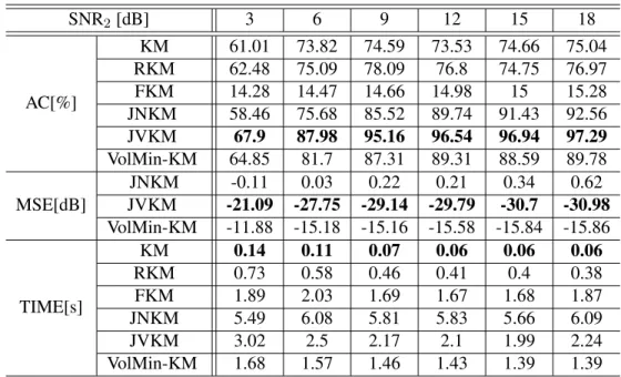
Table 2.2 presents the clustering accuracies of various algorithms usingI = 50,J = 1000,

F = 7, andK= 10. The MSEs of the estimatedWˆ of the factorization-based algorithms are

also presented. We set the parameters of the JNKM method to beλ= 1,µ= 100andη = 10−1.

Here, SNR1is fixed to be 15 dB and SNR2varies from 3 dB to 18 dB. The JNKM is initialized

with an NMF solution [74], and the JVKM is initialized with the SISAL [15] algorithm. We

see that, for all the SNR2’s under test, the proposed JNKM yields the best clustering accuracies.

RKM and FKM give poor clustering results since they cannot resolve the distortion brought by

W, as we discussed before. Our proposed method works better than NMF-KM, since JNKM

estimatesH more accurately (cf. the MSEs of the estimated factorW) – by making use of the

cluster structure onHas prior information.

Note that in order to make the data fit the VolMin model, we normalized the columns ofX

to unit`1-norm as suggested in [48]. Due to noise, such normalization cannot ensure that the

data follow the VolMin model exactly, however we observe that the proposed JVKM formulation still performs well in this case.

To better understand the reason why our method performs well, we present an illustrative

(44)

Table 2.2: Clustering and factorization accuracy for identifiable NMF vs. SNR2, forI = 50, J = 1000, F = 7, K = 10, SNR1 = 15dB. SNR2[dB] 3 6 9 12 15 18 AC[%] KM 77.43 81.5 82.9 81.47 82.68 84.5 RKM 77.51 76.62 73.71 72.43 71.35 71.63 FKM 15.12 15.68 16.6 17.14 37.5 59.74 JNKM 88.1 95.12 96.51 96.13 96.43 95.65 JVKM 75.84 83.87 87.87 89.96 90.27 89.36 NMF-KM 84.72 86.62 88.96 90.95 90.87 92.34 MSE[dB] JNKM -28.09 -27.82 -27.54 -26.59 -26.91 -26.26 JVKM -16.41 -16.98 -16.37 -15.61 -15.19 -14.9 NMF-KM -27.09 -26.75 -26.7 -25.58 -26.05 -25.31 TIME[s] KM 0.14 0.05 0.05 0.07 0.06 0.06 RKM 0.18 0.13 0.16 0.17 0.17 0.18 FKM 1.45 0.59 0.64 0.79 0.82 0.56 JNKM 3.37 2.99 3.13 3.22 3.06 3.36 JVKM 5.7 5.06 4.73 4.53 4.42 4.45 NMF-KM 0.76 0.68 0.73 0.83 0.75 0.86

Table 2.3: Clustering and factorization accuracy for identifiable NMF vs. SNR1, forI = 50, J =

1000, F = 7, K = 10, SNR2 = 10dB. SNR1[dB] 5 10 15 20 25 30 AC[%] KM 78.65 77.89 82.89 84.53 88.43 86.97 RKM 79.54 72.84 72.87 71.15 71.37 72.06 FKM 17.91 17.3 16.76 16.68 16.44 16.51 JNKM 93.28 94.69 95.73 96.33 96.43 96.04 JVKM 71.78 82.74 87.43 91.68 92.43 93.17 NMF-KM 84.95 86.74 89.57 90.87 90.66 91.61 MSE[dB] JNKM -18.03 -23.95 -26.71 -27.17 -27.09 -26.19 JVKM -4.66 -12.19 -15.96 -20.21 -25.14 -31.05 NMF-KM -17.63 -23.36 -26.29 -27.48 -27.76 -27.13 TIME[s] KM 0.08 0.08 0.05 0.05 0.04 0.04 RKM 0.18 0.18 0.16 0.14 0.11 0.11 FKM 0.68 0.7 0.66 0.69 0.61 0.67 JNKM 3.1 3.29 3 3.13 2.99 2.92 JVKM 3.21 3.83 4.57 5.12 5.01 4.94 NMF-KM 0.74 0.75 0.7 0.66 0.64 0.62

(45)

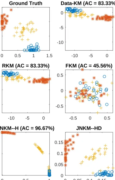
0 0.5 1 1.5 0 0.5 1 1.5 Ground Truth -10 -5 0 -10 -5 0 Data-KM (AC = 83.33%) -10 -5 0 -10 -5 0 RKM (AC = 83.33%) -0.5 0 0.5 -0.5 0 0.5 FKM (AC = 45.56%) 0 0.5 1 0 0.5 1 JNKM--H (AC = 96.67%) 0 0.05 0.1 0.15 0 0.05 0.1 0.15 JNKM--HD

Figure 2.3: Illustration of how linear transformation obscures the latent cluster structure, and

how identifiable models can recover this cluster structure. Top left: true latent factorH; Top

right: data domainX =W H+E1, visualized using SVD (two principal components); Middle

left: projected data found by RKM,PTX; Middle right: projected data found by FKM,PTX;

Bottom left:H found by JNKM; Bottom right:HDfound by JNKM. In the top right subfigure,

the clustering accuracy of running K-means directly on the data is shown; for other figures, the clustering accuracy given by corresponding method is shown.

(46)

Table 2.4: Simulation comparison of the clustering methods, identifiable NMF model.I = 50, F = 7,J = 100K. K 5 6 7 8 9 10 11 AC[%] RKM 79.97 78.57 76.6 76.16 75.48 75.22 75.54 FKM 47.75 34.01 27.32 21.96 18.45 16.55 15.14 JNKM 97.6 97.5 97.43 97.37 96.88 96.63 95.48 MSE[dB] JNKM -4.7 -7.52 -25.08 -24.77 -24.3 -24.17 -23.81

and has a clear cluster structure. The basisW is an8×2matrix. The factor are generated such

that the NMF model is identifiable. Fig. 2.3 shows the true latent factors, together with those

found by various methods. Clearly,W brings some distance distortion to the cluster structure in

H (cf. top right subfigure). We see from this example that if the factorization model is

identi-fiable, using the proposed approach helps greatly in removing the distance distortion brought

byW, as indicated by the last row of Fig. 2.3. On the other hand, the other semi-orthogonal

projection-based algorithms do not have this salient feature.

Table 2.3 presents the results under various SNR1’s. Here, we fix SNR2= 10dB, and the

other settings are the same as in the previous simulation. We see that the clustering accuracies are

not so sensitive to SNR1, and the proposed JNKM outperforms other methods in AC and MSE

in most of the cases. Table 2.4 presents the ACs and MSEs for fixed rankF = 7as the number

of clustersKvaries from5to11. HereI = 50,J = 100K, SNR1 = 6dB, and SNR2 = 8dB.

We observe that the performance of all methods degrades when we add more clusters, which is expected. However, RKM and FKM suffer more than the proposed method.

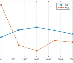
In Fig. 2.4, we show the effect of changingλin the JNKM formulation. We are particularly

interested in this parameter since it plays an essential role in balancing the data fidelity and prior

information. On the other hand, the parameterµfor enforcingZto be close toHcan be set to

a large number, e.g., 1000, andηfor balancing the scaling of the factors can usually be set to

a small number – and the algorithm is not sensitive to these two according to our experience.

(47)

are set to SNR1 = 5dB and SNR2 = 30dB. From Fig. 2.4, we see that both the MSE and AC

performance of JNKM is reasonably good for all theλ’s under test, although there does exist a

certainλgiving the best performance (λ= 3000in this case).

0 1000 2000 3000 4000 5000 6000 6 70 75 80 85 90 AC -12 -11 -10 -9 -8 MSE AC MSE

Figure 2.4: AC and MSE versus parameterλ

So far we have been working with sparse nonnegative factors. Let us consider a generalW

and aHwith columns in a simplex, i.e.1TH =1T, H ≥0, which finds various applications

in machine learning, e.g., document and hyperspectral pixel clustering / classification [48, 47].

We generateH using the same steps as in the previous simulations with the centroid matrix

M(:, k)’s being generated by putting a cluster near each unit vector, and several centroids

randomly; under such setting, the identifiability conditions of the VolMin model are likely to

hold [44]. Note that the entries ofW are simply drawn from a zero-mean unit-variance i.i.d.

Gaussian distribution, which means thatW is a dense matrix and the identifiability of NMF

does not hold – which differs from the previous simulations. Table 2.5 presents the results. We see that JNKM works worse relative to the previous simulation, since the generative model is not identifiable via NMF. However, JVKM works quite well since the VolMin identifiability holds

(48)

Table 2.5: Clustering and factorization accuracy for identifiable VolMin vs. SNR2, for I = 50, J = 1000, F = 7, K = 10. SNR2[dB] 3 6 9 12 15 18 AC[%] KM 61.01 73.82 74.59 73.53 74.66 75.04 RKM 62.48 75.09 78.09 76.8 74.75 76.97 FKM 14.28 14.47 14.66 14.98 15 15.28 JNKM 58.46 75.68 85.52 89.74 91.43 92.56 JVKM 67.9 87.98 95.16 96.54 96.94 97.29 VolMin-KM 64.85 81.7 87.31 89.31 88.59 89.78 MSE[dB] JNKM -0.11 0.03 0.22 0.21 0.34 0.62 JVKM -21.09 -27.75 -29.14 -29.79 -30.7 -30.98 VolMin-KM -11.88 -15.18 -15.16 -15.58 -15.84 -15.86 TIME[s] KM 0.14 0.11 0.07 0.06 0.06 0.06 RKM 0.73 0.58 0.46 0.41 0.4 0.38 FKM 1.89 2.03 1.69 1.67 1.68 1.87 JNKM 5.49 6.08 5.81 5.83 5.66 6.09 JVKM 3.02 2.5 2.17 2.1 1.99 2.24 VolMin-KM 1.68 1.57 1.46 1.43 1.39 1.39

MSE performance of VolMin and NMF.

In Table 2.6, we test the joint tensor factorization and latent clustering algorithm (JTKM).

We generate a three-way tensorX ∈ _RI×J×L _with_I ₌ _J ₌ _L _{= 30} _{and loading factors}

A ∈ _RI×F_, _B _∈

RJ×F, C ∈ RL×F. To obtainA with a cluster structure on its rows, we

first generate a centroid matrixM = 2I+11T, and then replicate its columns and add noise

to createA˜. This way, the rows ofA˜randomly scatter around the rows ofM. Then we let

A =DA˜, whereDis a diagonal matrix whose diagonal elements are uniformly distributed

between zero and one. Here,BandC are randomly drawn from an i.i.d. uniform distribution

between zero and one. Gaussian noise is finally added to the obtained tensor. As in the matrix

case, SNR1denotes the SNR in the data domain, and SNR2the SNR in the latent domain. In this

experiment we set SNR1 = 20dB, SNR2 = 25dB. As before, to create more severe modeling

error so that the situation is more realistic, we finally replace two slabs (i.e.,X(:,:, i)’s) with

(49)

Table 2.6: MSE and clustering accuracy of JTKM vs. NTF for variousF =K. F 2 3 4 5 6 7 8 AC[%] JTKM 92.97 74.17 72.33 74.2 76.93 78.4 79.47 NTF 80.5 64.8 62 62.63 62 62.2 62.7 MSE[dB] JTKM -22.54 -12.45 -10.04 -10.81 -12.08 -12.92 -13.84 NTF -21.52 -11.51 -9.66 -10.47 -11.53 -12.28 -13.34

commonly seen in practice.

We apply the tensor version of the formulation in (2.14) to factor the synthesized tensors for

variousF =K. For each parameter setting, 100 independent trials are performed with randomly

generated tensors, and the results are the average of all these trials. As shown in Tab. 2.6, the proposed approach consistently yields higher clustering accuracy, and lower MSEs than plain NTF. This suggests that the clustering regularization does help in better estimating the latent factors, and yields a higher clustering accuracy.

To conclude this section, we present a simulation where the latent data representations lie in different subspaces. We apply the joint factorization and latent subspace clustering algorithm to deal with this situation. As a baseline, the latent space sparse subspace clustering (LS3C) method [102] is employed. The idea of LS3C is closely related to FKM, except that the latent clustering part is replaced by sparse subspace clustering. We construct a dataset with data that lie in two

independent two-dimensional subspaces. We setI = 10,J = 200,F = 4andK = 2; each

subspace contains 100 data columns. As before, we add noise in the latent domain, as well as

the data domain. The SNR in data domain is fixed at SNR1 = 30dB, and the SNR in the latent

domain varies. The parameters of our formulation are set toλ= 1andµ= 0.5. For LS3C, we

used the code and parameters provided by the authors5. The results are shown in Table 2.7. As

can be seen, our method recovers the factors well, and always gets higher clustering accuracy.

5