Title: Computation of Lagrangian Coherent Structures with
Application to Weak Stability Boundaries
Author: Xavier Ros Roca
Advisor: Francesco Topputo
Department: Dipartamento di Scienze e Tecnologie
Aerospaziali, Politecnico di Milano
Co-Advisor: Mercè Ollé Torné
Department: Departament de Matemàtica Aplicada I
Academic year: 2014 - 2015
Universitat Politècnica de Catalunya
Facultat de Matemàtiques i Estadística
Bachelor’s Degree Thesis
Computation of Lagrangian Coherent
Structures with Application to Weak
Stability Boundaries
Xavier Ros Roca
Advisor: Francesco Topputo
1Co-advisor: Mercè Ollé Torné
21.
Dipart. di Scienze e Tecnologie Aerospaziali - Politecnico di Milano
2.
Departament de Matemàtica Aplicada I - UPC
Als meus avis, als dos els hauria agradat llegir aquesta tesi
Abstract
Key words: ordinary differential equations, non-linear dynamics, Lagrangian coherent struc-tures, celestial mechanics, elliptic three body problem
MSC 2010: 34C99, 37C10, 70F07, 70F15, 70K99
Real-life mechanical systems can usually be modeled as linear, periodic and non-autonomous dynamical systems. It is very important to have different tools to study these systems, and there are many classical procedures developed for this purpose. During the last decade, a new tool has been introduced, the Lagrangian Coherent Structures (LCS). They represent the most repelling and attracting structures of the phase space. Roughly speaking, LCS are particular manifolds that separate regions of space with distinctly different dynamics. In this thesis, algorithms to find the LCS of a system are presented and finally they will be applied in theElliptic Restricted Three Body Problemin Astrodynamics in order to identify theWeak Stability Boundaries.
Acknowledgements
First of all, I would like to thank my advisors in Politecnico di Milano, Francesco Topputo and Alex Wittig. They invested a lot of their time in this thesis, meeting every Tuesday. I am very grateful to them for their scientific support and their warm host during these 6 months in Milan. Grazie mille!
També vull agrair profundament a la Mercè Ollé, professora de la Univeristat Politèc-nica de Catalunya i co-tutora d’aquest Treball de Fi de Grau, per donar-me l’excel·lent contacte del Francesco a Milà. Valoro molt també la lectura desinteressada amb ull crític de la tesi per part seva.
Quiero agradecer también a Ana, Mario e Inés por las horas invertidas en el proyecto en la sala de tesistas en Milán, elhacer un café de media mañana, eltris para comer en la cafetería de Bovisa y también que me acogieran siempre en Ingegnoli 5 cenando el mejorkebab de Milán.
Vull fer especial menció als meus companys de carrera, tant el grup de Findus com els amics de la FME i de l’ETSEIB, per aquests magnífics 5 anys universitaris i les mil experiències viscudes. Així com al CFIS i el seu equip directiu i administratiu per la oportunitat i dedicació durant aquests anys.
La major part del TFG ha estat elaborada a Milà, per tant, vull donar les gràcies també als amics d’Erasmus com la Laura, l’Alba i el Carlos amb el nostre magnífic viatge i, sobretot, a Carolina y Fer por su buena amistad y grandes momentos en Milán, habéis sido una pieza fundamental.
Finalment, fer especial menció a gent que m’ha ajudat molt durant l’elaboració del TFG com l’Uri Castejón, amb la resolució de dubtes tècnics en sistemes dinàmics, a la Paula, pels infinits Hangouts Amsterdam-Milà i a la Marina per hores d’escriptura junts i consells tècnics. Sense oblidar-me òbviament dels meus pares, la meva germana i gent molt especial com l’Albert, l’Anna, el Jaume, la Glòria i el Raül i un llarg etcètera. Gràcies a tots de debò!
Contents
1 Introduction 1
1.1 Motivation . . . 1
1.2 Brief History of LCS . . . 2
1.3 Introduction to Dynamical Systems . . . 3
2 Lagrangian coherent structures 7 2.1 Characteristics of an LCS . . . 7
2.2 The finite-time Lyapunov Exponents . . . 9
2.3 The Variational LCS theory . . . 11
3 Computation of LCS 17 3.1 Computation of FTLE fields . . . 17
3.2 LCS-finder inspired by the Variational theory . . . 19
3.2.1 The strainlines . . . 20
3.2.2 The region U0 . . . 22
3.2.3 LCS candidate;LCS . . . 24
3.3 Analogous results of Attracting LCS . . . 28
4 Application to the ER3BP 31 4.1 Weak Stability Boundaries . . . 31
4.1.1 Elliptic Restricted Three Body Problem . . . 31
4.1.2 Weak Stability Boundaries . . . 33
4.2 Adaptation to LCS Theory . . . 37
4.2.1 Hypothesis . . . 37
4.2.2 The system . . . 38
4.2.3 Methodology . . . 39
4.3 Results and Analysis . . . 41
4.4 Future Developments . . . 43
1
Introduction
This chapter introduces the main topic of this thesis, theLagrangian Coherent Struc-tures. The motivations for studying this new field in non-linear dynamical systems will be given. Secondly, some research history will be explained and to finish this chapter, there will be some preliminary definitions and results of Dynamical Systems.
1.1
Motivation
The study of Dynamical Systems, the study of their behavior with respect to initial conditions, in the case of autonomous, time-periodic and quasi-periodic systems is very complete and rigorous. In those systems, one can study the fixed points, the in-variant manifolds and, from these inin-variant objects, one can also study the qualitative behavior of all the system.
In contrast, all these techniques are not applicable in non-autonomous and aperiodic systems and the reality is that no fluid particle in the ocean or atmosphere will be part of a periodic orbit. Historically, there are many procedures such as linearization or modern heuristic diagnostics to try to obtain some information of the Lagrangian point of view of these systems, [9].
This thesis studies a new technique to try to understand the real-life systems math-ematically. This new approach tries to show the transport pattern of the system through the most repelling, attracting and shearing structures of the system. These structures will be what is called Lagrangian Coherent Structures, shortly LCS. An LCS must act as separatrix of regions with qualitatively different dynamics, [13]. To turn this characteristic to a mathematical definition took many years and approaches that are shown in this thesis.
The applications in fluid dynamics of this new concept are remarkable. In2010 two globally significant events occurred. In April, a volcanic eruption in Iceland caused chaos in the European airspace. The same month, there was an explosion in the Gulf of Mexico causing the largest offshore oil spin in the US. In addition, in March2011, a tsunami in Japan caused a nuclear-reactor disaster and the release of amounts of radioactive contamination in the Pacific ocean. As explained in [18], further analysis showed that finding the attracting and repelling LCS of these three significant events would have been useful to forecast future situations of the disasters and to take better decisions. This informative article ensures that LCS will be a very powerful
2 1. Introduction
tool when computation and data storage improve in many fields such as biological fluids, industrial and chemical transports.
One last objective of this thesis is to find a new application of LCS in Astrodynamics. The repelling Lagrangian coherent structures will be used as an alternative to find the Weak Stability Boundaries (WSB) in the elliptic restricted three body problem
(ER3BP). Roughly speaking, WSB is a boundary of a region near the planet where capture of the third particle occurs, [21]. This technique was developed during the
80s and proved in 1991when Japanese satellite Hiten was able to reach the Moon, [21]. The WSB is useful to find what it is called as low-cost transfers to reach a planet, [2], because the particle is ballistically captured, ie, the object makes, under natural dynamics within the sphere of influence of that planet, at least one complete revolution around the planet, [12].
1.2
Brief History of LCS
At the beginning, the aim of the researchers that work on this topic was to find what they named as the skeleton of the fluid, which are some structures that will give an idea of the pattern and shape of the flow after an interval of time. The term of Lagrangian coherent structure was coined by G. Haller and G. Yuan in [10] in
2000. This name was used for defining the most attracting and repelling material surfaces of the system. The immediate application of this new concept is to find some separatrices in the phase space, in the case of the most repelling structures, or to find, for example, the area where there will be more concentration of a substance after a while, in the case of the attracting LCS.
A lot of theories have been developed during these 15 years, [7, 8, 15]. The main researchers and developers are George Haller and his research group established in Zurich, Thomas Peacock from MIT and Shawn Shadden from Berkeley University. Those last two researchers dedicated their research on stochastic dynamical systems andG. Haller works on continuous dynamical systems focused on unsteady flows. From 2005 to 2010, LCS has not had a mathematical definition. Firstly they were defined as the ridges of Finite-Time Lyapunov Exponents field (FTLE), [8, 15], but in 2010, G. Haller in [8] realized that FTLE field ridges were not corresponding to the repelling LCS and turned the physical definition into a mathematical definition. Furthermore, he developed a mathematical, and rigorous, theory of LCS around the invariants of Cauchy-Green strain tensor field. In this remarkable paper, he also established the sufficient and necessary conditions for the existence of LCS and a new way to find them.
From 2010, their research is focused on new theory in higher-dimensional flows and on obtaining new efficient methods to find LCS, [3, 5, 6, 9]. The future research has to be focused on finding an efficient implementation to ease the obtaining of LCS because it will be a useful tool to forecast future states in all kind of flows.
1.3. Introduction to Dynamical Systems 3
1.3
Introduction to Dynamical Systems
The main definition of a Dynamical System is taken from [17], which defines it as a
rule for time evolution on a state phase, using more formal vocabulary:
1.3.1 Definition (Dynamical System) ADynamical Systemis a system that evolves in time. This system is formed by a state space S, a set of times T and a rule
R:S×T →S which describes the evolution of the state in time.
Thestate spaceis a set of coordinates needed to describe completely the system. This space is going to change in time, so therule will predict the next state or states. It can be discrete or continuous. When it’s continuous, it is usually a smooth manifold intoRn and it’s called phase state.
The set of times can be also discrete, for example in an ideal coin toss dynamics, or continuous. In the case of being continuous, it can be assumed as an interval
I= [α, β]⊆R.
Finally therule is an application that describes the future state or states of a coor-dinate in S. For a states0∈S, the orbit ortrajectory is the time-ordered sequence
of states using therule.
Along this thesis, LCS are studied only in Dynamical Systems where the state space and the time space are both continuous. Furthermore, the phase state should be a manifold into a finite dimensional space. One can model these systems as a general Ordinary Differential Equations’ Cauchy problem:
˙ x(t) = f(x(t), t) x(t0) = x0 x(t) ∈ Ω⊆Rn t ∈ I= [α, β] (1.1)
where tis the independent variable that represents the time and x(t)represents the state of the system at time t. The field f : Ω×I → Ω is a sufficiently smooth field called thevelocity map. Traditional assumptions in fluid mechanics, [20], ask to
f(x(t), t) to be at leastC0 in time and C2 in space. From that, it follows that the
flowφt
t0(x)will beC
1 in time andC3 in space.
Equivalently, one can define the evolution of a Dynamical System through theflow map, which is defined below.
1.3.2 Definition (Flow map) Fort0, t∈I, we can define the flow map as
φt
t0 : Ω→ Ω
x07→ φtt0(x0) =x(t;t0,x0)
Theflow map satisfies the following properties for anyx∈Ω: 1) Identity
φt0
4 1. Introduction 2) Group property φtt+0s(x) =φts+s(φts0(x)) =φtt+s(φtt0(x)) 3) Differentiability dφt t0(x) dt =f(x(t), t)
1.3.3 Proposition (Variational equations) Consider any initial conditions x0 ∈ Ω
andt∈I in a Dynamical System of the form of (1.1). Then, given a fixed timet∈I, the following ordinary differential equations system is satisfied, recalling
Φ := Φ(t;t0,x0) =Dx0φ t t0(x0) , A(x, t) =Dxf(x, t) then ˙ Φ = A(x, t) Φ Φ(t0;t0,x0) = Idn
whereIdnis then-dimensional identity matrix,Φ = Φ(t;t0,x0)is thestate transition
matrix of the system and Ais the Jacobian of the velocity field. If one joins the two systems
˙ x(t) = f(x(t), t) x(t0) = x0 x(t) ∈ Ω⊆Rn ˙ Φ = A(x, t) Φ Φ(t0;t0,x0) = Idn t ∈ I= [α, β] (1.2)
This system is called theVariational equationsof the system and it isn+n2−dimensional.
The variational equations are useful to find the Jacobian of the flow,Φ, that will be essential in this thesis.
1 Proof The flow satisfies the differential equation (1.1), so we have
d dtφ t t0(x0) =f t,φ t t0(x0)
By deriving the equality with respect to the initial conditionx0
Dx0 d dtφ t t0(x0) =Dx f t,φtt0(x0) Dx0φ t t0(x0)
By Cauchy-Schwarz theorem, the derivatives order in the left hand side can be changed
d dt Dx0φ t t0(x0) =Dx f t,φtt0(x0) Dx0φ t t0(x0) so then, as wanted ˙ Φ =A(x, t)·Φ
For the initial condition, it’s only necessary to derive the first property of the flow with respect to the initial conditions
Dx0φ t0
1.3. Introduction to Dynamical Systems 5
2
One important object in this thesis is the finite-time Cauchy-Green strain tensor
which shows the average deformation of the infinitesimal neighborhood after a finite-time interval. As an operator, it will be a very useful tool to find the maximum stretching direction at every point.
1.3.4 Definition (Finite-time Cauchy-Green strain tensor) Letx1(t0)∈Ωbe a
par-ticle in the phase space andx2(t0) =x1(t0) +δx(t0)at the initial time. After a time
intervalT, these points will bex1(t0+T)andx2(t0+T). Then, by first order Taylor
expansion, δx(t0+T) =φtt00+T(x2)−φ t0+T t0 (x1) = Φ·δx0+O(kδx0k 2 )
whereΦis the state transition matrix for a finite timet0+T. The norm of this vector
δx(t0+t)indicates the distance of the two particles afterT.
kδx(t0+T)k 2
=hΦ·δx0,Φ·δx0i= δxT0 ·Φ
T ·Φ·δx
0=δxT0 ·∆·δx0
where the Cauchy-Green tensor is∆(T;x0, t0) := ΦT ·Φ. The notation∆ := ∆(t0+
T;x0, t0)andΦ := Φ(t0+T;x0, t0)will be used along all the thesis.
By construction, one can easily see that∆is symmetric and positive definite because it comes from a distance definition. Thus, it hasnreal positive eigenvalues that can be ordered as
0< λ1≤ · · · ≤λn
Theseneigenvalues and their nassociated eigenvectors indicate the stretching mag-nitude on each direction. When λi<1, the system is compressing at the associated
direction. Otherwise, whenλi>1, the system is expanding. The maximum stretching
will be at the associated eigenvectorξn of the maximum eigenvalue,λn.
Figure 1.1: Ellipsoid of the Cauchy-Green tensor in a2D−system. The length of the unit vectorsξ1 andξ2 become
√
λ1and
√
6 1. Introduction
Further information of the system can be extracted from this tensor. Due to the fact that the tensor is symmetric and positive definite, the eigenvectors are orthogonal and they turn the infinitesimal sphere around x0 into an ellipsoid as in Figure 1.1.
Moreover, one can notice that the system is area-preserving when the product of all the eigenvalues is equal to 1, expanding when it is greater than 1 and compressing when it is less than1.
One last definition is needed for this thesis. This is the notion ofmaterial surface.
1.3.5 Definition (Material surface) A Material surface is denoted by M(t) and it is a manifold of the phase space Ω×[α, β], generated by the advection of an n−1 -dimensional manifoldM(t0)⊂Ωby the flow map. So then:
M(t) =φtt0(M(t0))
Equivalently, and more understable, oneMaterial surfaceis one manifold of the phase space at the initial time,M(t0), that is advected by the flow until a finite time. Hence,
M(t0)is evolving with the flow. Sinceφtt0 is a diffeomorphism, the material surface
at timet is as smooth as the initial surfaceM(t0)and it isn−1-dimensional,∀t.
As shown in next chapter, an LCS must be a material surface as it is written in Proposition 2.1.1.
2
Lagrangian coherent
structures
The aim of this chapter is to collect all the theory developed around the LCS. The historical development of the theory will be followed in this chapter. Therefore, first the Finite-Time Lyapunov Exponent (FTLE) field and it’s relation with the LCS is introduced, followed by the newer Variational LCS theory.
This chapter is very influenced by [8] where G. Haller makes a deep review of the theory obtained until2010and develops rigorously the Variational LCS theory, which corresponds to Section2.3 in this thesis.
2.1
Characteristics of an LCS
Complex dynamical systems are usually very sensitive to changes in their initial condi-tions. This makes the classification of dynamical regimes where orbits behave similarly hard to do by the classical methods. Behind these complex and sensitive patterns, however, there exists a robust skeleton of special material surfaces calledLagrangian coherent structures.
The worldLagrangiancomes from the fact that these structures must evolve with the flow, as a material surface does. The words coherent structures mean that they are regions of the flow that are distinguishable in time and space and separate different dynamics of the flow.
First results in LCS theory demonstrate that these structures were full separatrices in the phase space through the time. Nevertheless, more recent investigations, [13, 15, 20], show that particles can cross the LCS and therefore that LCS separate regions that have qualitatively different dynamics. That is, LCS act as the most important barriers to mixing of scalar fields such as dye concentrations in fluids.
2.1.1 Proposition As proposed in [10], LCS are expected to have two key properties: 1) An LCS should be a material surface, as given in 1.3.5, because it must have sufficient dimension to have a visible impact and must move with the flow to act as a transport barrier.
2) An LCS should present locally the strongest attraction, repulsion or shearing forces in the flow.
8 2. Lagrangian coherent structures
Recalling classical invariant manifolds classification in autonomous dynamical sys-tems, LCS can also be classified in three categories:
Hyperbolic LCS: The most attracting and repelling structures.
Elliptic LCS: Closed material surfaces.
Parabolic LCS: The strongest shearing structures.
In this thesis, only hyperbolic LCS are going to be studied in depth.
Based on the key properties that an LCS must satisfy, one can give a purely physical definition:
2.1.2 Definition (Physical Definition of Hyperbolic LCS) A Hyperbolic LCS over a finite time-interval I = [α, β] is a locally strongest repelling or attracting material surface overI.
Figure 2.1: Hyperbolic LCS. Capture from [8].
This definition captures the main physical property of a hyperbolic LCS but there is no mathematical definition that allows computing LCS in dynamical systems. Two different mathematical approaches that had been developed until now will be given in this chapter, the first one is related to the FTLE field and the second is called
Variational LCS theory.
Simple counterexamples in [8] reveal conceptual problems in the first theory and thus, the second theory explained below was developed. Despite that, FTLE remain useful as a popular and visual tool to see the global repulsion behavior in complex dynamical systems.
2.2. The finite-time Lyapunov Exponents 9
2.2
The finite-time Lyapunov Exponents
In this section, the theory around the Finite-time Lyapunov exponents field and it’s correlation with LCS is going to be explained. This theory was developed between
2002and2010in [15, 16, 20].
2.2.1 Definition (Finite-time Lyapunov Exponents field) The field calledFinite-time Lyapunov Exponents (FTLE) is the fieldσtT0 :D⊆R
n → Rdefined by σTt 0(x) = 1 |T|ln p λn(∆)
whereλn(∆)is the largest eigenvalue of the Cauchy-Green Tensor defined in (1.3.4).
For the remainder of this section, in order to avoid degeneracy and non-regularity in the FTLE field, [15, 20], it will be assumed that 0 < λi <1, i = 1,· · ·, n−1, and
λn>1. Adding the assumption from Definition 1.1, one can ensure thatσtT0(x)isC
2
in space andC1in time and that LCS aren−1−dimensional material surfaces, [20].
Given this field that measures the maximum expansion rate for a pair of near particles by the advection of the flow, the authors of [15] and [20] agreed in describing repelling LCS as theridges of the FTLE field.
In the2−dimensional phase space case, it is easy to find theridges of the FTLE field by visual inspection because it’s graph is a surface inR3. So that, one can easily find
the repelling LCS by inspection in FTLE plots such the one below:
Figure 2.2: Classic FTLE plot for a2−dimensional plot. (grid: 200×200)
In Figure 2.2, one can intuit the ridges of the field plotted in red. According to this theory, those ridges plotted in red are the repelling LCS of the Dynamical System over
10 2. Lagrangian coherent structures
the interval[t0, t0+T]. In that cases, one can parameterize the LCS by interpolation
methods of the formγ : (a, b)→Ω⊆R2 because it is1−dimensional. To generalize
the idea of LCS as ridges of the FTLE field inn−dimensional dynamical systems, one can use the notion of second derivative extrema. So then,
2.2.2 Definition (Repelling LCS) Arepelling LCS is a codimension1, orientable and differentiable manifoldM ⊂Ω⊆Rnsatisfying the following conditions for each point
x∈ M:
1) The unit normal vectorn(x)to the manifoldMis orthogonal to∇σtT0(x).
2) LetΣ =Dx2σTt0(x0)be the Hessian matrix ofσ T
t0(x), thought as a bilinear form
evaluated at x, we require:
Σ(n,n)<0
and
Σ(n,n)<Σ(u,u)
for all unit vectorsusuch thathu,ni 6=±1.
Orientation ofMis needed to ensure the uniqueness of the normal vectorn(x).
2.2.3 Definition (Attracting LCS) Anattracting LCSis a repelling LCS of the backward-time flow, i.e. when integration backward-time goes fromt0+T to t0.
As said before, the FTLE field as tool to find hyperbolic LCS presents some incon-sistencies in some dynamical systems. In fact, G. Haller in [8], subsection2.3, gave some simple and relevant examples that show that FTLE theory is not good enough. To summarize the information obtained by these three examples:
1) Observed LCS are not necessarily ridges of the FTLE field, as one can notice in the non-linear saddle flow system (example 1 in [8]). This shows that the association of LCS to FTLE ridges is not always correct. In the cases of saddle flows, symmetry at the LCS gives wrong results.
2) Ridges of FTLE field are not necessarily Hyperbolic LCS. FTLE field presents ridges also to indicate important shearings, which are parabolic LCS. In fact, this procedure ignores if the direction ξn associated to the largest eigenvalue
is close to the tangent direction of M(t0), which provokes shearing instead of
repelling deformation.
3) FTLE ridges could break the2 key properties of Proposition 2.1.1. The proper-ties ofcoherence andLagrangian are important by definition.
In conclusion, the FTLE ridges are an heuristic procedure to find LCS. Hence, one does not have the certainty of the results obtained. However, this procedure is visual and fast, compared to the Variational LCS theory. Therefore, it is essential to know when it is applicable. In general, it can be used as support for quick estimations and preliminary designs.
2.3. The Variational LCS theory 11
2.3
The Variational LCS theory
In order to solve the inconsistencies given by the last examples,G. Haller presented the mathematical theory that is going to be developed in the next section. This new theory is used to develop the LCS finding algorithms. This section is based on sections
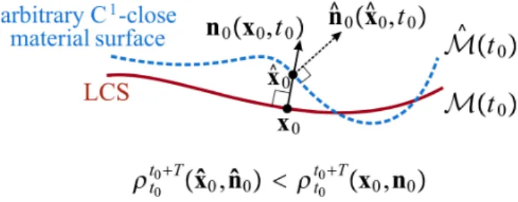
3 and4of the article [8] and its correction [4], byG. Haller andM. Farazmand. Consider an arbitrary material surface M(t) ⊂ Rn. As defined, this manifold is
n−1−dimensional, hence, at an initial point x0 ∈ M(t0), one can consider the
tangent space,Tx0M(t0), and the normal space,n0:=Nx0M(t0),n−1−dimensional
and1−dimensional respectively. Those two spaces can be advected by the linearized flow mapDx0φ t t0(x0), as shown: M(t0);φtt0(M(t0)) Tx0M(t0);Dx0φ t t0(x0)Tx0M(t0) n0;Dx0φ t t0(x0)n0
By properties of the linearized flow map, the tangent space is advected to the tangent space ofM(t)atxt=φtt0(x0). By contrast, the advected normal vector is generally
not coincident to the normal spacent:=NxtM(t), as can be seen in Figure 2.3.
Figure 2.3: Advection of M(t0), Tx0M(t0), and n0. Capture from [8], where
∇Ftt0(x0)≡Dx0φ t t0(x0).
Thus,Dx0φ t
t0(x0)n0has a general orientation on the space and can be expressed as
following: Dx0φ t t0(x0)n0=ρ t t0(x0,n0)·nt+π t t0(x0,n0)·TxtM(t) 1 Remark πt t0(x0,n0) is the projection ofDx0φ t
t0(x0) n0 at TxtM(t)called the net
shear ofM(t)over a finite-time interval.
2.3.1 Definition (Repulsion rate) The projection of Dx0φ t
t0(x0) n0 to the unitary
normal space ofM(t)atxtis called therepulsion rateand it’s denoted byρtt0(x0,n0):
ρtt0(x0,n0) =nt, Dx0φ t
t0(x0)n0
12 2. Lagrangian coherent structures
The repelling and attracting nature of the surface is captured by this parameter.
ρt
t0(x0,n0) > 1 indicates that the normal component of normal perturbations to
M(t0)grows by time. Similarly, whenρtt0(x0,n0)<1 indicates average attraction at
the normal direction.
2.3.2 Definition (Repulsion ratio) The ratio between normal and tangential growth after a finite-interval time is
νtt 0(x0,n0) = |emin 0|= 1 e0∈Tx0M(t0 ) nt, Dx0φ t t0(x0)n0 Dx0φ t t0(x0)e0 Then, νt
t0(x0,n0) >1 indicates that infinitesimal normal growth along M(t)
dom-inates the largest tangential growth. In that case, M(t) is the locally dominant repelling structure atx0.
The next proposition gives a manner to compute and estimate ρt
t0 and ν
t
t0 in terms
of the Cauchy-Green strain tensor.
2.3.3 Proposition The quantities defined above can be computed and estimated as follows: 1) Computation: ρtt0(x0,n0) = 1 p hn0,∆−1 n0i νtt 0(x0,n0) = |emin 0|= 1 e0∈Tx0M(t0 ) ρt t0(x0,n0) p he0,∆e0i
where∆−1stands for the inverse matrix of∆(x
0, t0, t), i.e. ∆−1:= ∆−1(x0, t0, t). 2) Estimation: p λ1(x0, t0, T)≤ρtt00+T(x0,n0)≤ p λn(x0, t0, T) s λ1(x0, t0, T) λn(x0, t0, T) ≤νt0+T t0 (x0,n0)≤ s λn(x0, t0, T) λ1(x0, t0, T)
where λ1 andλn are the lowest and the greatest eigenvalues of∆(x0, t0, T).
2 Proof The proof of Proposition 2.3.3 can be found in section3.1of [8].
2
Right now, it’s possible to define one set of material surfaces, those that are normally repelling or attracting over a time interval. Inside this subset, one can find the most normally repelling or attracting material surfaces, calledHyperbolic LCS.
2.3. The Variational LCS theory 13
2.3.4 Definition (Normally repelling (attracting) material surface) Given a mate-rial surface M(t) ⊂ Ω, it is normally repelling over [t0, t0 +T] if for all points
x0∈ M(t0)and unit normaln0,
ρt0+T
t0 (x0,n0)>1, ν t0+T
t0 (x0,n0)>1
are satisfied.
Similarly, M(t)isnormally attracting over [t0, t0+T]if it’s normally repelling over
in backward time. Both of them can be also called hyperbolic material surface over
[t0, t0+T].
ρt0+T
t0 (x0,n0) >1 indicates normal stretches in x0. ν t0+T
t0 (x0,n0) >1 ensures that
any tangential deformation along M(t)is strictly smaller than the repelling force in the normal direction.
2.3.5 Definition (Hyperbolic LCS) A normal repelling (attracting) material surface M(t)is called arepelling (attracting) LCS over [t0, t0+T]if its normal repulsion rate
admits a pointwise non-degenerate maximum along M(t0) among all locally C1−
close material surfaces.
Figure 2.4: LCS definition as an extremum surface for the normal repulsion rate.
2 Remark The mathematical point of view of Definition 2.3.5 is asking to accomplish the non-degenerate relative minimum condition at any pointx0∈ M(t0):
∂ ∂ερ t0+T t0 (xε(t0),nε(t0))|ε=0= 0 ∂2 ∂ε2ρ t0+T t0 (xε(t0),nε(t0))|ε=0<0
wherexε(t0) =x0+εα(x0, t0)n0(t0)andα(x0, t)is an appropiate smooth function.
Choosing an appropiate continuous (with respect tox0) functionα(x0, t0), one
con-structs all theC1−close material surfaces.
After defining the concept of Hyperbolic LCS, one has to set the sufficient and nec-essary conditions that ensure the existence of an LCS. [8] gives the most important theorem (Theorem 7) of the Variational LCS theory. Based on that theorem, The-orem 2.3.6 gives a clear relation between LCS and the invariants of the finite-time Cauchy-Green strain tensor.
14 2. Lagrangian coherent structures
2.3.6 Theorem (Sufficient and necessary conditions for an LCS) Given a compact material surface M(t) ⊂ Ω ⊂ Rn over the interval [t0, t0+T]. Then, M(t) is a
repelling LCS over[t0, t0+T]if and only if all the following hold for allx0∈ M(t0):
1) λn−1(x0, t0, T)6=λn(x0, t0, T)>1
2) ξn(x0, t0, T)⊥Tx0M(t0)
3) hDx0λn(x0, t0, T), ξn(x0, t0, T)i= 0
4) The matrix L(x0, t0, T) ∈ Mn(R), see Matrix 2.1, is positive definite for all
x0∈ M(t0)
whereλi andξi are the eigenvalues and the eigenvectors of ∆(x0, t0, T).
L(x0, t0, T) = D2x0∆ −1 [ξn] 2λn−λ1 λ1λn hξ1, Dx0ξnξni · · · 2 λn−λn−1 λn−1λn hξn−1, Dx0ξnξni 2λn−λ1 λ1λn hξ1, Dx0ξnξni 2 λn−λ1 λ1λn · · · 0 . . . ... . .. ... 2λn−λn−1 λn−1λn hξn−1, Dx0ξnξni 0 · · · 2 λn−λn−1 λn−1λn (2.1)
where the first term is
Dx2 0∆ −1[ξ n] =− 1 λ2 n ξn, Dx20λnξn + 2 n−1 X q=1 λn−λq λnλq hξq, Dx0ξnξni 2
3 Remark Matrix L(x0, t0, T) comes from the proof of the theorem. It has no
ex-plicit meaning, it’s just a way to put some inequalities in order using Sylvester cri-teria for positive definiteness. Moreover, future developments will show that matrix
L(x0, t0, T) will be never computed in 2−dimensional systems, another equivalent
condition will be established in proposition 2.3.7.
3 Proof A scheme of the proof is shown below. This proof was made by G.Haller’s group in [8]. Further details and the complete proof can be found in [8], section 4.1, with some corrections in Erratum [4].
1st step Prove that condition(1),(2)and(3) are necessary:
The extremum property of the repulsion rate along M(t)is going to be formulated. For that, a C1−material surface nearby M(t), Mε(t) is constructed by the same
development used in remark 2, pointsxε(t0)∈ Mε(t)are of the form:
xε(t0) =x0+εα(x0, t0)n0(t0)
with an appropiate smooth functionα: Ω×I→Ω. Imposing,
∂ ∂ερ
t0+T
2.3. The Variational LCS theory 15
some developments that are shown by detail in [8], using Proposition 2.3.3 and Taylor developments ofnε(t0)aroundn0, one arrives to
n X i,j=1 n−1 X p=1 ∆−ij1(x0)eipn j 0= 0 (2.3) n X i,j,k=1 ∆−ij,k1(x0)ξniξ j nξ k n= 0 (2.4)
where∆−ij,k1 is the differentation of∆ij−1with respect toxk,uiis thei−th component
of the vectoruandep,p= 1,· · ·, n−1form an orthonormal basis of Tx0M(t0).
By differentiating the eigenvalue problem of ∆−1 with respect toxk, and using the
identityPn
i=1ξ
i nξ
i
n= 1and its differentation, one obtains: n X i,j=1 ∆−ij,k1ξniξjn=−λn,k λ2 n
which implies, using equation (2.4), hDx0λn,ξni= n X k=1 λn,kξnk =−λ 2 n n X i,j,k=1 ∆−ij,k1(x0)ξniξ j nξ k n= 0
so then, condition(3)of the theorem is necessary.
Note that equation (2.3) implies directly ∆−1n0⊥Tx0M(t0), which is condition (2).
Equivalently, ∆−1n
0||n0, which states that n0 must be an eigenvector of∆−1.
Defi-nition 2.3.4 forcesn0to beξnand the corresponding eigenvalueλn to be multiplicity
one, which makes condition(1)necessary (adding thatνt t0 >1).
2nd step Prove that condition(4)is necessary:
To prove condition (4), one has to ensure to have a non-degenerate local maximum ofρtt0 inn0 direction, so then
∂2
∂ε2ρ
t0+T
t0 (xε(t0),nε(t0))|ε=0<0 (2.5)
Procedures similar to those on step 1, that can be found in [8], prove that (4) is needed to be an LCS.
3rd step Conditions are also sufficient:
Applyingξn ≡n0, result obtained in 1st step, in Proposition 2.3.3, one deduces:
ρt0+T t0 = p λn>1 νt0+T t0 = s λn λn−1 >1
That results holding for all x0 ∈ M(t0) implies that M(t0) is a normally repelling
material surface. Furthermore, we have seen that(1),(2)and(3)derive from Equation 2.2 and proved the sufficiency of that conditions. Finally, the positive definiteness of
L(x0, t0, T)guarantees that Equation 2.5 is satisfied. Hence, the four conditions are
16 2. Lagrangian coherent structures
2
4 Remark In the 3rd step of the proof, new ways to compute ρt0+T
t0 andν
t0+T
t0 have
been found when M(t) is an LCS. The new value of ρt0+T
t0 =
p
λn(x0, t0, T)is the
maximal value that it can take because of the Estimation given in Proposition 2.3.3. Next chapter is dedicated to the computation of LCS in continuous 2−dimensional dynamical systems. Therefore, Theorem 2.3.6 in 2−dimensional dynamical systems can be re-written as follows, in order to avoid to compute the matrix L(x0, t0, T).
2.3.7 Proposition (Sufficient and necessary conditions for Hyperbolic LCS) Given a compact material surfaceM(t)⊂Ω∈R2which is arepelling LCS over the interval [t0, t0+T]. Then: 1) λ1(x0, t0, T)=6 λ2(x0, t0, T)>1 2) ξ2(x0, t0, T), Dx20λ2(x0, t0, T)ξ2(x0, t0, T) <0 3) ξ2(x0, t0, T)⊥Tx0M(t0) 4) hξ2(x0, t0, T), Dx0λ2(x0, t0, T)i= 0
4 Proof Conditions(1),(3)and(4)came directly from theorem 2.3.6. Condition(2)
derives from the application of Sylvester’s criteria to the matrix L(x0, t0, T), which
asks to the leading principal minors ofLto be positive, so then:
Dx20∆−1[ξn] =− 1 λ2 2 ξ2, Dx20λ2ξ2 + 2λ2−λ1 λ1λ2 hξ1, Dx0ξ2ξ2i 2 >0 (2.6) detL= 2λ2−λ1 λ1λ2 Dx20∆−1[ξn]− 2λ2−λ1 λ1λ2 2 hξ1, Dx0ξ2ξ2i>0 (2.7)
From inequality 2.6 one derives to hξ1, Dx0ξ2ξ2i 2 > λ1 2λ2(λ2−λ1) ξ2, Dx20λ2ξ2 (2.8) and from inequality 2.7
−2λ2−λ1 λ1λ32 ξ2, D2x0λ2ξ2 >0 (2.9) Inequality 2.9 is equivalent toξ2, Dx20λ2ξ2
<0becauseλ2> λ1>0. Finally, using
this last inequality in 2.8, one arrives to condition 2, as desired.
2
Proposition 2.3.7 will be used to define new objects and properties that will be useful to construct an algorithm to do it computationally.
3
Computation of LCS
This chapter is dedicated to the computation methods to find LCS in2−dimensional Dynamical Systems, so then, n= 2in all the chapter. Furthermore, the assumption ofλn−1<1< λn applies also in this chapter, so that, λ1<1 < λ2. In this section,
only algorithms for the Repelling LCS are designed. One final section in this chapter gives some analogous results to Attracting LCS.
Algorithms to find the LCS by the two different methods studied are given, firstly the FTLE visualization algorithm, based on [20], and secondly the Variational Theory, [5].
As mentioned, the first theory is not conclusive and will be used only to see the patterns. Second theory will be used to develop an LCS-finder algorithm given any
2D−Dynamical System
The content of this chapter will be applied in one typical example in non-linear dy-namics,the Double Gyre. This system was chosen in order to compare all the results obtained with the results shown in [5] which influenced the algorithmics of this thesis.
3.1
Computation of FTLE fields
This section is dedicated to the computation of the finite-time Lyapunov exponents field (FTLE). The first step is to calculate the Cauchy-Green tensor and its eigenvalues
λ1<1< λ2and the associated eigenvectorsξ1,ξ2. For the remainder of this chapter,
the nomenclature E ={λ1, λ2,ξ1,ξ2} will be used to call the quartet of eigenvalues
and eigenvectors of∆, the Cauchy-Green strain tensor.
Given a Dynamical System of the form of Equation 1.1, let x0 ∈ Ω ⊆ R2 be an
arbitrary point and let [t0, t0+T] ⊂[α, β] be the finite-time interval of integration,
by Runge-Kutta methods, one can integrate theVariational Equations:
˙ x(t) = f(x(t), t) x(t0) = x0 ˙ Φ = A(x, t) Φ Φ(t0;t0,x0) = Idn x(t) ∈ Ω⊆R2 t ∈ I= [α, β] (3.1)
18 3. Computation of LCS
in order to find the Jacobian of the flow,Φ := Φ(t0+T;t0,x0).
5 Remark The Jacobian of the flow,Φ, after a finite-time interval can also be com-puted by central finite differences, taken from section4.1 in [19]. Partial derivatives of a function can be approximated by:
∂fi
∂xj
≈ fi(x+hej)−fi(x−hej)
2h
By this method, one has to integrate4n= 4·2 = 8Ordinary Differential Equations (ODEs). On the other hand, using the Variational Equations given in 3.1 one has to integrate one system ofn+n2= 2 + 22= 6ODEs.
Note that these ODEs are different to the ones of the other method. Therefore, it is not assured that the Variational Equations are more efficient than central finite differences.
Once Φ is obtained, the Cauchy-Green strain tensor is calculated by ∆ := ∆(t0+
T;t0,x0) = ΦT·Φand its quartetE is computed with an eigenvalue problem solver.
The FTLE field requires the value of the greatest eigenvalueλ2, as shown in Definition
2.2.1. Onceλ2 is calculated, one can easily compute the FTLE field.
The algorithm to compute the FTLE graphics is the following:
Algorithm 1FTLE visualization algorithm
% G0⊂Ωis the grid of initial conditions in the phase space. % [t0, t0+T]is the interval of integration.
while x0∈ G0 do
ObtainingΦby integration of the System 3.1
∆ := ΦT ·Φ
ObtainingE={λ1, λ2,ξ1,ξ2}by an eigenvalue solver.
σt0+T t0 (x0) := 1 |T|ln p λ2(∆) Plotσt0+T t0 (x0), ∀x0∈ G0.
3.1.1 Example (The Double Gyre) The Double Gyre is a2−dimensional non-linear dynamical system given by the equations:
( x˙ = −Aπsin(πf(x, t)) cos(πy) ˙
y = Aπcos(πf(x, t)) sin(πy)∂f
∂x(x, t)
(3.2)
where
f(x, t) =a(t)x2+b(t)x a(t) =εsin(ωt) , b(t) = 1−2 a(t)
andA, ε, ω arbitrary parameters. The phase space is Ω = [0,2]×[0,1]and the time interval I= [0,∞). In this computation, the parameters used are A= 0.1, ε= 0.1,
ω= 2π/10,t0= 0andT = 20, the same values in [5] in order to compare the results
3.2. LCS-finder inspired by the Variational theory 19
(a) Obtained numerically. (grid: 200×100) (b) Taken from [5].
Figure 3.1: FTLE plots of the Double Gyre.
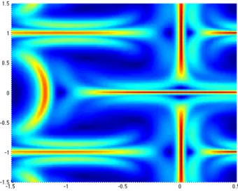
Figure 3.1a shows the forward-time FTLE plot of the Double Gyre. This plot was obtained numerically with Algorithm 1. Red corresponds to the highest values of the FTLE field. Analogously, blue corresponds to the lowest values. Thus, one can easily detect the ridges of the FTLE field, in red. Recalling Definition 2.2.2, they are the repelling LCS of the system.
As explained in section 2.2, this plot shows an idea of the dynamics of the system but not always the ridges correspond to the repelling LCS. Despite that, the computation is very easy and fast so the computation of this plot gives a preliminary idea of the most repelling areas in the phase space over[t0, t0+T]. Further information will be
obtained with the implementation of the Variational theory, shown in next section.
3.2
LCS-finder inspired by the Variational theory
The algorithms of this section follow the ideas given in [5]. The intention in this section is to create an LCS-finder from the Variational LCS theory as explained in the cited article.
Remembering Proposition 2.3.7, which gives the sufficient conditions to a material surface for being an LCS, it is necessary to state an efficient algorithm to find the LCS of the phase space.
One should remark the difficulty of computing the4 statements of Proposition 2.3.7 due to their numerical sensitivity. Computing the quartet E implies ODE solvers, numerical differentation and eigenvalue problem solvers. After that, one has to com-pute more derivatives in order to verify the 4 necessary conditions. As given in [5] in section II.B, Proposition 2.3.7 can be reformulated as given below so as to have a more robust implementation:
3.2.1 Proposition (Relaxed Proposition 2.3.7) Given a curveΓ(t0)⊂Ω⊂R2which
20 3. Computation of LCS (A) λ1(x0, t0, T)=6 λ2(x0, t0, T)>1 (B) ξ2(x0, t0, T), D2x0λ2(x0, t0, T)ξ2(x0, t0, T) <0 (C) ξ1(x0, t0, T)||Tx0Γ(t0)
(D) λ¯2(Γ(t0)), the average ofλ2 over the curve, is maximal among all nearby curves
γ(t0)such thatγ(t0)||ξ1(x0, t0, T).
6 Remark Note that in2−dimensional phase spaces,Tx0Γ(t0)is1−dimensional and
it is spanned by the tangent vector of the curve Γ(t0)at the pointx0∈Γ(t0).
5 Proof Comparing those two Propositions (2.3.7 and 3.2.1), one can notice that first and second conditions did not change.
Condition (3) has been changed to (C) using the orthogonality ofξ1andξ2due to the
spectral theorem of linear algebra and using also thatTx0Γ(t0)is the tangent vector
of the curveΓ(t0), see Remark 6.
Condition (4) has been relaxed using the fact that n0 =ξ2(x0, t0, T) and ρtt00+T =
p
λ2(x0, t0, T)>1 if x0 ∈LCS, results taken from the proof of the Theorem 2.3.6,
and: d dερ t0+T t0 (x0+εξ2,ξ2)|ε=0= 1 2pλ2(x0, t0, T) hξ2(x0, t0, T), Dx0λ2(x0, t0, T)i= 0
This result says that the repulsion rate is a maximum onξ2 direction for all nearby
curves. That allows to relax condition (4), of Proposition 2.3.7, to condition (D), of Proposition 3.2.1.
2
The design of the final algorithm to find LCS uses Proposition 3.2.1. Sufficient con-ditions to be a repelling LCS are given and the key is to find a manner to compute all of them efficiently. For this reason, next sections give some results and ideas that will approach us to the final Algorithm 3.
3.2.1
The strainlines
From condition (C) of Proposition 3.2.1, one can notice that the LCS are those curves,
Γ(t0), tangent toξ1, the eigenvector associated to the smallest eigenvalue,λ1,∀x0∈ Γ(t0). So then, there’s a new set of curves in the phase space:
3.2.2 Definition (Strainline) Given a Dynamical System of the form 1.1 and a finite-time interval I = [t0, t0+T]. A strainline is a curve γ(t0) ⊂Ω such that it is the
orbit of the Cauchy problem:
x0(s) = ξ1(x(s), t0, T) x(0) = x0∈Ω |ξ1| = 1 (3.3)
where ξ1 = ξ1(x(s), t0, T) stands for the smallest eigenvector calculated at x ∈ Ω
3.2. LCS-finder inspired by the Variational theory 21
Hence, the LCS set is the subset of the strainlines that satisfies conditions (A), (B) and (D) of Proposition 3.2.1.
In order to be more efficient numerically, an appropiate scaling in the velocity map of System 3.5, suggested in [5], is presented:
x0(s) = ξ˜1(x(s), t0, T)
x(0) = x0∈Ω
(3.4)
whereξ˜1(x(s), t0, T) =sign(x(s))α(x(s))ξ1(x(s), t0, T)is the product of these3maps:
ξ1(x(s), t0, T)is the eigenvector of the Cauchy-Green strain tensor computed as
in Algorithm 1.
Functionα(x(s))is needed to stop the solver when approaching possible degen-erate points. It is computed as follows:
α(x(s)) = λ
2(x(s))−λ1(x(s))
λ2(x(s)) +λ1(x(s))
2
where λi(x(s))are the eigenvalues of the Cauchy-Green strain tensor, that are
computed as in Algorithm 1.
sign(x(s))ensures the smoothness of the trajectory. Given the tangent vector of
γ(t0)atx(s), ifuis parallel toγ0(t0), then−uis also parallel toγ0(t0). At each
step of the integration, xk, this function takes the sign of the following inner
product hξ1(xk, t0, T),xk−1−xki. Hence, it ensures that the right eigenvector
is chosen to guarantee the smoothness of the curve: hξ1(xk, t0, T),ξ1(xk−1, t0, T)i ≥0
As one can notice right now, computing a strainline is also expensive computationally because, for each evaluation of the right-hand side of 3.4, the ODE of the Dynamical System has to be solved fromt0 tot0+T in order to obtain the quartetE.
7 Remark Function α(x(s)) ensures also that Condition (A) is satisfied because it stops the solver in the case that there’s a degenerate point.
8 Remark As suggested in [5], small LCS have negligible effect on the phase space evolution. To filter out that curves, one parameter is created as a minimum length allowed to be a strainline. This parameter islmin.
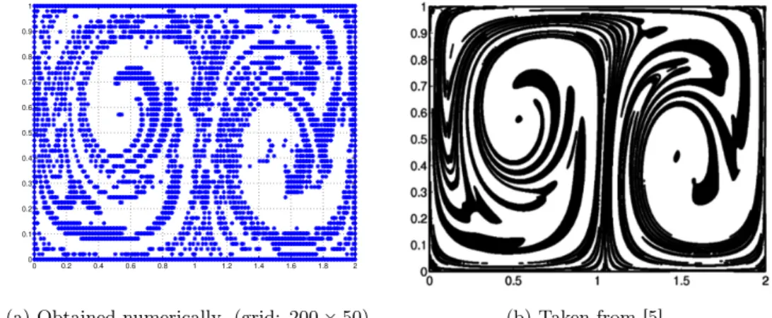
3.2.3 Example (The Double Gyre) Using the same example than before, Example 3.1.1, the strainlines are computed, as trajectories of the Cauchy Problem 3.4, and shown in Figure 3.2a. Recalling Remark 8,lmin= 1, as in [5].
22 3. Computation of LCS 0 0.2 0.4 0.6 0.8 1 1.2 1.4 1.6 1.8 2 0 0.1 0.2 0.3 0.4 0.5 0.6 0.7 0.8 0.9 1
(a) Obtained numerically. (grid: 50×25) (b) Taken from [5].
Figure 3.2: Strainlines of the Double Gyre.
Subfigures from Figure 3.2 show the strainlines of the Double Gyre. On the left, Figure 3.2a, there is the graph obtained computationally with Algorithm 3, using an ODE solver to integrate equations 3.4. On the right, Figure 3.2b, is a capture from the example followed in [5]. Even though the number of strainlines is different, one can see the similarity of the plots.
Those strainlines from Figure 3.2a that satisfy Conditions (B) and (D) of Proposition 3.2.1 will be repelling LCS. To find the LCS, the grid used will be 8 times thiner,
200×50.
3.2.2
The region
U
03.2.4 Definition (RegionU0) Given a Dynamical System of the form 1.1 and a
finite-time intervalI = [t0, t0+T]. Theregion U0 ⊆Ωis the region where Condition (B)
of Proposition 3.2.1 is satisfied, so then: U0= x0∈Ω : ξ2(x0, t0, T), D2x0λ2(x0, t0, T)ξ2(x0, t0, T) <0
whereξ2(x0, t0, T)is the eigenvector associated to the largest eigenvalueλ2(x0, t0, T)
andD2x0λ2(x0, t0, T)is the Hessian of the field λ2(x0, t0, T).
Computing regionU0is expensive computationally and extremely sensitive. For each
pointx0∈ G0, the trajectory fromt0tot0+T has to be calculated in order to obtain
E = {λ1, λ2,ξ1,ξ2}. After that, the Hessian must be computed. And finally, one
should compute the inner product.
9 Remark The Hessian can be computed by double finite differences, see Remark 5, or by other more complex methods. The accuracy of the region U0 depends on the
method used.
In this thesis, a MATLAB code, extracted from [1], is used. This code is in File Exchange Matlab website, which works as a sharing-codes place. It is made by John D’Errico, who is in theTop 10 Authors of that website with55codes and more than
3.2. LCS-finder inspired by the Variational theory 23
Even though double finite differences to compute the Hessian was the fastest proce-dure, it was discarded because of its low accuracy.
As seen in Figures 3.4, regionU0 is very sensitive to the procedure used to compute
the Hessian of λ2(x0, t0, T)and to the grid used. The grid size and the tolerance of
the ODE solver are two elements that must be well-adjusted in order to reduce the computation time without losing accuracy.
10 Remark Recalling Proposition 3.2.1, condition (B) must be fulfilled for all the points of an strainline in order to be an LCS candidate. For that reason, Algorithm 3 considers only pointsx0∈ U0as initial condition for the strainlines.
While computing the strainline, the inner product must be negative for all pointsxk
of the ODE solver. In order to make faster the LCS-finder algorithm, double linear interpolation is used.
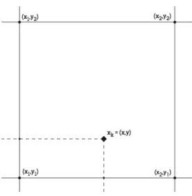
Letxk ∈Ωbe a point of a strainline obtained by using an ODE solver. Then,xk is
framed by4points of the grid, as seen in Figure 3.3. The inner product of condition (B) is calculated by double linear interpolation with the points of the grid with the formula that follows:
f(xk)≈
1
(x2−x1)(y2−y1)
[f(x1, y1)(x2−x)(y2−y) +f(x2, y1)(x−x1)(y2−y)+ +f(x1, y2)(x2−x)(y−y1) +f(x2, y2)(x−x1)(y−y1)]
Figure 3.3: Double Linear Interpolation.
11 Remark As suggested in [5], in order to avoid accidentally failures due to numerical errors computing the inner product of condition (B), another filter parameter is used. This parameter is lf and it is the maximum length of a part of the curve where
computed condition (B) is not satisfied. It will be always less than a20%of the other filter parameterlminfrom Remark 8.
24 3. Computation of LCS
3.2.5 Definition (LCS candidate) For the remainder, a strainline that satisfies con-dition (B), with the filter parameter of Remark 11, is called anLCS candidate. If an
LCS candidate satisfies also condition (D), then it is an LCS.
3.2.6 Example (The Double Gyre) Using the same example than before, Example 3.1.1, with the filter parameter lf = 0.2. The regionU0 is computed as explained in
this subsection. 0 0.2 0.4 0.6 0.8 1 1.2 1.4 1.6 1.8 2 0 0.1 0.2 0.3 0.4 0.5 0.6 0.7 0.8 0.9 1
(a) Obtained numerically. (grid: 200×50) (b) Taken from [5].
Figure 3.4: RegionU0of the Double Gyre.
Subfigures from Figure 3.4 show the region U0 of the Double Gyre. On the left,
Figure 3.4a, there is the graph obtained computationally. On the right, Figure 3.4b, is a caption from the example in [5]. As can be seen in Figure 3.4, the accuracy of the computation affects to the regionU0, the graph obtained from [5] is made with a
grid of1000×500.
3.2.3
LCS candidate
;
LCS
Let Γ(t0) = {x0,· · ·,xfinal} be an LCS candidate computed using an ODE solver,
condition (D) from Proposition 3.2.1 states:
“λ¯2(Γ(t0)), the average of λ2 over the curve, is maximal among
all nearby curvesγ(t0)such thatγ(t0)||ξ1(x0, t0, T).”
The algorithm designed to check condition (D) uses the fact that the quartet E was necessarily computed for all the points of the LCS candidates,xk. Then, given a step
parameter ε >0, two parallel curves are created as follows:
γ+(t0) :={x+0,· · · ,x + final}, wherex + i =xi+εξ2 γ−(t0) :={x−0,· · ·,x − final}, wherex − i =xi−εξ2
3.2. LCS-finder inspired by the Variational theory 25
Then, the average values of λ2 field over the three curves, Γ, γ+, γ−, are calculated
by Λ2(γ)≈ Pi=final i=1 λ2(xi)· kxi−1−xik Pi=final i=1 kxi−1−xik
which is a simple numerical aproximation, [19], for the average of the field over the curve: Λ2(γ) = R γλ2dγ R γ1 dγ
Once the average quantities are calculated, an LCS candidate becomes an LCS if
Λ(Γ(t0))is the maximum. This subsection is summarized in Algorithm 2.
Algorithm 2LCS candidate ;LCS
% Γ(t0)∈ U0⊂Ω⊆R2 is a strainline that satisfies condition (B). % [t0, t0+T] is the interval of integration.
% Γ(t0) ={x0,· · ·,xfinal}. It is a set of points because it is computed numerically. % length(γ) :=Pi=final
i=1 kxi−1−xikcomputes the length of the curveγ.
% int(λ2(γ(t0))) :=Pii==1finalλ2(xi)· kxi−1−xik computes the integral ofλ2 field % over the curveγ.
% εis a step parameter, as small as desired.
whilei= 0÷finaldo
% E was obtained during the computation of the strainline, Section 3.2.1.
x+i =xi+εξ2 x−i =xi−εξ2 end while γ+(t0) :={x+0,· · · ,x + final} γ−(t 0) :={x−0,· · ·,x − final} Λ2:=int(λ2(Γ(t0))/length(Γ(t0)) Λ+2 :=int(λ2(γ+(t0))/length(γ+(t0)) Λ−2 :=int(λ2(γ−(t0))/length(γ−(t0)) if Λ2>Λ+2 andΛ2>Λ−2 then Γ(t0)is an LCS. end if
3.2.7 Example (The Double Gyre) Using the same example than before, Example 3.1.1, with the filter parameters lmin = 1 and lf = 0.2. The repelling LCS are
computed with Final Algorithm 3. Figure 3.5 shows the differences between the plot obtained by the computation in this thesis and the plot taken from [5].
26 3. Computation of LCS 0 0.2 0.4 0.6 0.8 1 1.2 1.4 1.6 1.8 2 0 0.1 0.2 0.3 0.4 0.5 0.6 0.7 0.8 0.9 1
(a) Obtained numerically. (grid: 200×50) (b) Taken from [5].
Figure 3.5: Repelling LCS of the Double Gyre.
As said many times in this chapter, Figure 3.5 proves that these developed algorithms are very sensitive to numerical errors. In that example, one can see that the results obtained in Figure 3.5a are very similar to those from the literature in Figure 3.5b, but there are many curves shown that shouldn’t be. Moreover, the LCS in the square of Figure 3.5b is not completely finished in the numerical obtention of Figure 3.5a. This means that more integration time for the System 3.4 may be needed in order to have longer strainlines.
Even the results given by the Algorithm 3 applied to the Double Gyre do not cor-respond exactly to those shown in [5], the similarity is clear. The numerical imple-mentation of the LCS theory is very sensitive to the relative and absolute tolerances in the ODE solvers and this has a relevant impact to the computation time because the ODE solver is used many times on any single strainline computation and on any computation of regionU0. Even more, the double linear interpolation implies carrying
more numerical errors to the final results. In this thesis, it has been decided to find an equilibria between admissible results and their computation time. More accuracy could have given better results but the time of computation would be too long.
3.2. LCS-finder inspired by the Variational theory 27
Algorithm 3LCS-finder inspired by Variational Theory
% Referred conditions (A), (B), (C), (D) are those from Proposition 3.2.1.
% G0⊂Ωis the grid of initial conditions in the phase space. % [t0, t0+T]is the interval of integration.
% U0⊆ G0⊂Ωis the set of the grid points that satisfies condition (B). % ode(f(xj, tj),xj)refers to an ODE solver that returns next pointxj+1 % where f(xj, tj)is the velocity map of the ODE.
% lf is the length allowed for (B) failures on strailines (See Section 3.2.1).
% lminis the minimum length allowed for an LCS. % length(γ) :=Pi=final
i=1 kxi−1−xikcomputes the length of the curveγ.
for all x0∈ G0 do
Check condition (B)%See Section 3.2.2
if x0∈ U0 then
whileL < lf do
% Find the Cauchy-Green strain tensor ∆(x0, t0, T) % Computation of strainlines, see Section 3.2.1
xj+1=ode( ˜ξ1(xj, sj),xj) if xj+1∈ U0then L:= 0 else L:=L+kxj+1−xjk end if end while if L≥lf then
It’s not an LCS candidate
else
LCScand:={x0,· · ·,xfinal}
if length(LCScand)≥lmin then
% Verify condition (D), see Section 3.2.3
doAlgorithm 2
end if end if end if end for
28 3. Computation of LCS
3.3
Analogous results of Attracting LCS
Chapter3in general is dedicated to the computation ofRepelling LCS. This section is dedicated to present, briefly, analogous results forAttracting LCS in2−dimensional Dynamical Systems. These last years,2013−2015, researchers have been dedicated to the computation of all kind of LCS, [6].
Recalling Definition 3.2.2 and the fact that an Attracting LCS is a Repelling LCS integrating in backward time, then:
3.3.1 Definition (Stretchline) A Stretchline is a strainline integrating ODE 3.4 in backward time.
As in the strainlines,stretchlines are the curves of the phase state that present more compressing forces than shearing forces at all points of the curve. Those that present locally most compressing forces than other stretchlines are theattracting LCS. So then, the stretchlines of a Dynamical System form the pattern of the attracting structures of the flow. Finding the stretchlines became easier from 2013due to this theorem, published and proved in [6].
3.3.2 Theorem dd
Forward time strainlines coincide with backward time stretchlines. Forward time stretchlines coincide with backward time strainlines.
From the proof of the Theorem 3.3.2, in Appendix A of [6], the next important corollary is deduced.
3.3.3 Corollary Given a Dynamical System of the form 1.1 and a finite-time interval
I = [t0, t0+T]. A stretchline is a curve γ(t0)⊂Ω such that is the orbit of the next
Cauchy problem: x0(s) = ξ2(x(s), t0, T) x(0) = x0∈Ω |ξ2| = 1 (3.5)
whereξ2=ξ2(x(s), t0, T)stands for the greatest strain eigenvector calculated atx∈Ω
integrating from t0 tot0+T.
This thesis is not going deeper through Attracting LCS. Chapter 4 will use only Repelling LCS. Table 3.6 is a summary of the ODEs that one has to solve in order to find this2 sets of curves:
Curves ODE
Strainlines x0(s) =ξ1(x(s), t0, T)
Stretchlines x0(s) =ξ2(x(s), t0, T)
(3.6)
Those two special curves of the Dynamical System indicate the repelling and attract-ing structures of the phase space. Evolvattract-ing them by time, one can have a general idea of the pattern of the flow after a finite-time interval.
3.3. Analogous results of Attracting LCS 29
Furthermore, Table 3.6 allows the simultaneous construction of attracting and re-pelling LCS over I = [t0, t0+T]from one single computation. This also makes the
4
Application to the
ER3BP
The objective of this chapter is to apply the concept studied in this thesis, the LCS, to a problem in Astrodynamics. The problem chosen is the computation of Weak Stability Boundaries (WSB) in theElliptic Restricted Three Body Problem (ER3BP) which is an important problem in space trajectories design.
First section is dedicated to the definition of the ER3BP and the Weak Stability Boundaries. In second section, the hypothesis and the methodology used are shown and, finally, the results of the application of the LCS theory are shown.
Finally, there is a section dedicated to possible further developments.
4.1
Weak Stability Boundaries
In spacecraft trajectories design, there is one special set of transfers from one planet to another, they are calledlow-energy transfers. These transfers are those which the spacecraft is ballistically captured by the gravitational field of the planet and, thus, propellant is not needed during the capture phase. This technique was used in1991
when one Japanese satellite, Hiten, reached the Moon using the gravitation forces of the Moon [21].
The technique consists in bringing the spacecraft to a certain point of the space with a certain velocity where it will be captured by the planet. TheWeak Stability Boundaries (WSB) are separatrices between those points of the space where the spacecraft is captured by the planet and those that escape naturally from the planet.
4.1.1
Elliptic Restricted Three Body Problem
The model taken is theelliptic restricted three body problem (ER3BP). In the ER3BP the motion of a massless particle,P3, is studied under the gravitational field generated
by the motion of two masses (the primaries),P1andP2, of massesm1andm2 (with
m1>> m2) respectively.
As the name says, the elliptic problem models the motion ofP2aroundP1 as elliptic
32 4. Application to the ER3BP
Their relative distance will therefore vary depending on the point in whichP2is found
in its elliptic orbit aroundP1, [21]. The solution of the two-body problem relative to
P1−P2 motion gives their distance,r:
r(f) = a(1−e 2)
1 +ecosf (4.1)
abeing the semi-major axis of the orbit ofP2aroundP1,eits eccentricity andf the
true anomaly as can be seen in Figure 4.1.
Figure 4.1: Elliptic orbit ofP2
The equations that describe the motion of the particleP3, relative to the normalized
co-rotating frame, under the gravitational field generated by the elliptic motion of the primaries, are, [21]: x00−2y0 =∂ω ∂x y00+ 2x0 =∂ω ∂y (4.2)
In this case, the derivates in the left term of the equations are not temporal, as there is a new independent variable that plays the role of time in the elliptic problem, the true anomaly,f. In the right terms of (4.2) appear the partial derivates of the potential,
ω, given by:
ω(x, y, f) = Ω(x, y) 1 +epcosf
,
being ep the eccentricity ofP2 orbit around P1 andΩthe potential function defined
as follows: Ω(x, y) = 1 2 x 2+y2 +1−µ r1 + µ r2 +1 2µ(1−µ) where r1 = p (x+µ)2+y2 and r 2 = p
(x+µ−1)2+y2 represent the distances
fromP3toP1andP2respectively, as in the scheme of Figure 4.2. On the other hand,
µ= m2
4.1. Weak Stability Boundaries 33
Figure 4.2: Elliptic orbit
The dependence of the true anomaly on time is, [11, 12]:
df dt =
(1 +epcosf)2
(1−e2
p)3/2
12 Remark The study of the ballistic capture trajectories involves orbits that can result in collision of P3 with either P1or P2. This fact implies a fail in the numerical
integration as there is a singularity in the System 4.2 whenr1,2→0. It is convenient
therefore to regularize the equations of motion in the vicinities of this limit, the regularization of Levi-Civita presents fairly good solutions to the problem. Further details of Levi-Civita methods can be found in [21].
4.1.2
Weak Stability Boundaries
Before explaining the meaning of stable sets and their computation it is important to defineballistic capture. As mentioned in [14],ballistic capture by a planet occurs when an object enters, under natural dynamics, within the sphere of influence of that planet and makes at least one complete revolution around it. This means that, in ballistic capture, additional energy does not need to be provided to the object and, therefore, no propellant has to be used in the maneuver. This savings of propellant can be useful later, for example, to stabilize the orbit once the satellite has been captured by the planet.
In the ER3BP the Kepler energy of the particle P3 relative toP2, which is the
me-chanical energy (kinetic and potential) of particleP3 considering onlyP2 attraction,
can be written as:
H2(f) = 1 2v 2 2(f)− µ r2 (4.3)
34 4. Application to the ER3BP
wherev2is the speed ofP3relative to aP2-centered inertial reference frame. In polar
coordinates it is expressed by:
v22(f) = r 2epsinf 1 +epcosf r20 +r22(1 + cosθ20)2 (4.4)
4.1.1 Definition (Ballistic Capture) Based on this Kepler energy, and considering
x(f)as a solution of (4.2), it is possible to define:
(a) Ballistic Capture: P3is ballistically captured byP2atf1if H2(x(f1))<0, and it
is temporarily ballistically captured (or weakly captured) byP2 if H2(x(f))<0
forf1 ≤f ≤f2 and H2(x(f))>0 for f < f1 and f > f2, for finite anomalies
f1< f2.
(b) Ballistic Escape: P3is ballistically ejected (or ballistically escapes) fromP2atf1
if H2(x(f))<0, forf < f1 and H2(x(f))≥0forf ≥f1.
l(
Figure 4.3: 1−stable and1−unstable trajectories
To verify the ballistic capture, the revolutions ofP3 aroundP2 are tracked. For this
reason, the trajectories with the following characteristics will be studied:
1) The initial position of the third particleP3is on a radial segmentl(θ2)departing
from P2 and making an angleθ2 with the x-axis of the synodic dimensionless
reference system. The trajectory is assumed to start at the periapsis of an oscullating ellipse around P2, whose semimajor axis lies on l(θ2) and whose
eccentricityeis fixed alongl(θ2). Thus, the initial distance fromP2is given by:
r2(f0) =a(1−e) (4.5)
where a and eare the major axis and the eccentricy of the ellipse orbit of P3
4.1. Weak Stability Boundaries 35
2) In theP2-centered frame the initial velocity of the particle is perpendicular to
l(θ2)and, as P3 is on the periapsis of its oscullating ellipse, the initial Kepler
energy is always negative,H2(f0)<0. In [11], the initial velocity ofP3is given
by the mapM:R2→ R4: M(r, θ) = r2=r θ2=θ r02= repsin(f0) 1 +epcos(f0) θ02= s µ(1 +e) r3(1 +e pcos(f0)) −1 (4.6)
3) OnceP3leaves the initial position onl(θ2), the equations of the ER3BP can be
integrated. According to the definition of ballistic capture and as can be seen in Figure 4.3, the motion is said to be n-stable ifP3 makesn turns around P2
and returns to l(θ2)on a point where its Kepler energy relative to the smaller
primary is negative, without having completed any revolution about P1 along
this trajectory. Otherwise the motion is said to ben-unstable. These can occur either if P3 makes at least one revolution about P1 (this situation is called
primary interchange escape) or if it returns to l(θ2) withH2 >0 after having
donen revolutions aboutP2.
4.1.2 Definition (n−stable sets) Given an ER3BP system with the fixed parameters
e, f0, fixed an angleθ2 ∈[0,2π], let l(θ2)be the radial segment, the n-stable set on
l(θ2)is defined as the countable union of open intervals:
Wn(θ2, e, f0) = [ k>1 r∗2k−1, r∗2k , (4.7) with r∗
1 = 0. Excepting r∗1, the points r∗2k, the upper limits of the intervals, are
n−unstable.
If these sets are computed for each value ofθ2 and fixed(e, f0), it is obtained:
Wn(e, f0) =
[
θ2∈[0,2π]
Wn(θ2, e, f0), (4.8)
and finally, ifWn(e, f0)are computed for a fixed value of eccentricitye, thecomplete
n-stable set is given by:
Wn(f0) =
[
e∈[0,1)
Wn(e, f0). (4.9)
13 Remark Note that
36 4. Application to the ER3BP
Now it is possible to define the Weak Stability Boundary (WSB) of order n that contains the set of points r∗(θ
2, e) along l(θ2) in which there is a change of the
stability of the trajectory.
4.1.3 Definition (Weak Stability Boundary (WSB)) Given an ER3BP system with a fixed true anomaly, f0. The Weak Stability Boundary (WSB) is the locus of all
points r∗(θ, e), for all radial lines l(θ2), at which there is a change of stability of
the initial trajectory. r∗ represents one of the endpoints of an interval(r∗2k−1, r∗2k), characterized by the fact that any r ∈ (r∗2k−1, r∗2k) gives a n-stable trajectory, and there exist r0 ∈/ (r2∗k−1, r2∗k) arbitrarily close to either r2∗k−1 or r2∗k that give a n -unstable solution. Its formal expression is:
∂Wn(f0) ={r∗(θ2, e)|θ2∈[0,2π], e∈[0,1)} (4.10)
(a)W1(0.90,0) (b)W2(0.90,0)
(c)W4(0.90,0) (d)W6(0.90,0)
Figure 4.4: n−stable sets of the Sun-Mars system. These graphs were obtained with the Data sets computed by the authors of [11].
Figure 4.4 shows some n−stable sets, in particular, the n−stable points of the Sun-Mars system are represented in black, forn= 1,2,4,6. The boundaries of the black sets are then−WSB of the system, i.e. ∂W1(0.90,0),∂W2(0.90,0),∂W4(0.90,0)and

![Figure 2.1: Hyperbolic LCS. Capture from [8].](https://thumb-us.123doks.com/thumbv2/123dok_us/11057968.2992648/20.892.278.627.547.831/figure-hyperbolic-lcs-capture-from.webp)
![Figure 2.3: Advection of M(t 0 ), T x 0 M(t 0 ), and n 0 . Capture from [8], where](https://thumb-us.123doks.com/thumbv2/123dok_us/11057968.2992648/23.892.247.696.600.765/figure-advection-m-t-t-x-m-capture.webp)