Cambridge-INET Working Paper Series No: 2019/18
Cambridge Working Papers in Economics: 1981
SEMIPARAMETRIC SINGLE-INDEX PREDICTIVE REGRESSION
Weilun Zhou
Jiti Gao
David Harris
Hsein Kew
(University of Cambridge) (Monash University) (University of Melbourne) (Monash University)
This paper studies a semiparametric single-index predictive regression model with multiple nonstationary predictors that exhibit co-movement behaviour. Orthogonal series expansion is employed to approximate the unknown link function in the model and the estimator is derived from an optimization under constraint. The main finding includes two types of super-consistency rates for the estimators of the index parameter. The central limit theorem is established for a plug-in estimator of the unknown link function. In the empirical studies, we provide ample evidence in favor of nonlinear predictability of the stock return using four pairs of nonstationary predictors.
Cambridge Working Papers in Economics
Faculty of EconomicsSemiparametric Single–index Predictive Regression
1
Weilun Zhou
†,
Jiti Gao
†,
David Harris
‡and
Hsein Kew
†† Monash University and ‡ University of Melbourne
September 2, 2019
Abstract
This paper studies a semiparametric single-index predictive regression model with multiple nonstationary predictors that exhibit co-movement behaviour. Orthogonal series expansion is employed to approximate the unknown link function in the model and the estimator is derived from an optimization under constraint. The main finding includes two types of super-consistency rates for the estimators of the index parameter. The central limit theorem is established for a plug-in estimator of the unknown link function. In the empirical studies, we provide ample evidence in favor of nonlinear predictability of the stock return using four pairs of nonstationary predictors.
Keywords: Predictive regression; Single-index model; Hermite orthogonal estimation;
Dual super-consistency rates; Co-moving predictors.
JEL classification: C13, C14, C32, C51
1The authors would like to thank Prof Chaohua Dong, Prof Oliver Linton, and Prof Peter C.B. Phillips for their constructive comments on earlier versions, and seminar participants of the Monash De-partment of Econometrics and Business Statistics and several conference participants at the 2018 China Meeting of the Econometric Society in Shanghai and the 2018 North American Summer Meeting of the Econometric Society at UC Davies for their useful comments. The first two authors also acknowledge the financial support by the Australian Research Council Discovery Grants Program under Grant Numbers: DP150101012 and DP170104421.
1
Introduction
Whether stock returns are predictable or not is a fundamental issue in finance. In the study of a standard predictive regression, predictability is examined in the context of a parametrically linear model:
yt=α+β×xt−1+et, (1.1)
whereytis the equity premium,xt−1is the lagged financial predictor andetis a martingale
difference sequence. The earliest method used in the literature to test predictability is to apply the conventionalt-test forβ. If the estimate of the slope coefficientβ is statistically significant, we can conclude that xt−1 is a significant predictor.
Although various empirical studies have been conducted to examine stock return pre-dictability (Fama and French, 1988; Goyal and Welch, 2003; Shiller et al., 1984; Welch and Goyal, 2008), this widely used linear predictive regression model may encounter two main problems (see Phillips,2015 for an overview of certain aspects of predictive regres-sion). The first problem is that several financial predictors are highly persistent or even nonstationary, yet the equity premium behaves like a stationary process. Therefore, a linear predictive regression model can be unbalanced because the time-series properties on both sides of the equation (1.1) are different. The second problem is that the paramet-rically linear models may not be robust to functional form misspecification. To address these two problems, Kasparis et al. (2015) proposed a nonparametric predictive regres-sion model and estimated it with a kernel-based method. Cai and Gao (2013) estimated this unknown function with Hermite functions—a sieve-based method.
However, practical implementation of these methods presents one major drawback—the methodology is restricted to the case of a scalar predictor only. Research on the multiple predictive regression model is limited in the literature, with one difficulty being the need to cope with multiple degrees of persistence of the predictors. Lamont (1998) suggested using dividend-price ratio (dp) and the payout ratio as predictors based on the conven-tional t-test. Ang and Bekaert (2007) found the predictability of the equity premium using both dividend yield (dy) and short rates according to the F test, with standard errors adjusted for the overlapping issue. In addition, Chen and Hong (2009) applied a smoothed kernel method on the predictive residuals to capture the potentially nonlinear
predictable component. Kostakis et al.(2015) proposed a testing procedure based on IVX estimation (self-generated instrument variables estimation)—which was first studied by Phillips and Magdalinos (2009)—and found some evidence regarding the short-horizon predictability of the equity premium. Recently, Xu and Guo (2019) proposed three new dimensionality-robust tests built on the IVX estimator. Their proposed tests can detect potential spurious predictability driven by existing tests that tend to over-reject the null of no predictability in a finite sample with a large model size. The methods discussed here are all based on parametrically linear models, while the nonlinear predictability of the equity premium using multiple predictors remains unknown.
To make our proposed model more balanced and allow for a potential nonlinear rela-tionship between the liner combination of comoving predictors and the dependent vari-able, we propose a semiparametric single-index predictive regression model of the form:
yt =g0(θ>0xt−1) +et, (1.2)
where xt = (x1,t, ..., xd,t)> is a vector of d-dimensional nonstationary time series, g0(.) is
an unknown univariate link function, θ0 is the single-index parameter such that ut−1 = θ0>xt−1 is stationary, and et is a martingale difference sequence. In terms of the
identifi-cation condition, we impose that kθ0k2 = 1 with a positive first element.
In a nonparametric multiple regression estimation context, researchers often encounter the curse of dimensionality problem. The single-index model considers a linear combina-tion of predictors that can capture the most informacombina-tion about the potentially nonlinear relationship between the dependent variable and the predictors; hence, this is an efficient way to solve the dimensionality problem.
Dong et al. (2016) (hereafter DGT) assumed that the single-index component ut =
θ0>xt was nonstationary based on the nonstationary assumption for xt. However, we
are more interested in the case in which ut−1 is stationary, and this is a natural way
to cope with the unbalanced issue we mentioned before. From an empirical point of view, many financial predictors exhibit co-movement behaviour (e.g., Figure 3 below shows the co-movement between dp and dy), and our proposed model can potentially consider this characteristic in the context of stock return predictability. In the literature for predictive regression with multiple predictors, Amihud et al. (2008) only considered
stationary predictors and Kostakis et al. (2015) assumed predictors with an arbitrary degree of persistence, yet excluded comoving predictors. Recently, Koo et al. (2016) proposed a Least Absolute Shrinkage and Selection Operator (LASSO) estimator in the presence of comoving predictors. In addition, Xu (2017) considered a linear predictive regression model allowing for both highly persistent and comoving predictors, and studied the behaviour of the proposed IVX test. To the best of our knowledge, no study is available for the single-index model when xt−1 is nonstationary yet ut−1 = θ0>xt−1 is
stationary.
In the literature for single-index models, H¨ardle and Stoker (1989) and Powell et al. (1989) proposed an average derivative estimation for the single-index parameter θ0. In
addition, there have been many papers (Ichimura, 1993; Powell et al., 1989; Xia, 2006) devoted to the estimation of single-index models based on the conventional nonpara-metric kernel-based method. Alternatively, the nonparanonpara-metric sieve-based approach has attracted great attention recently in the literature to approximate unknown functions (see Chen,2007for a detailed review). Yu and Ruppert (2002) proposed penalised spline estimation for partially linear single-index models. Dong et al. (2015) proposed consis-tent closed-form estimators for both the single-index parameter and the unknown link function, based on Hermite expansion.
This paper studies the estimation of model (1.2) using Hermite polynomials. Although ut−1 =θ0>xt−1 is considered a stationary process, the nonstationarity of each regressor is
harder to deal with than the pure stationary case. Some recent work byPark and Phillips (2000) and DGT employed the so-called rotation technique to decompose the estimator into two directions: alongside and orthogonal to the direction of the true parameter θ0.
We adopt the same technique to develop the theory. However, in contrast with these two previous papers, we assume u1t−1 =θ>0xt−1 is stationary, rather than nonstationary, and
need to ensure that the nonstationary component will not dominate and the stationarity onut−1 will not break down.
To ensure the identification requirements we discussed before, the relevant literature uses the estimate θbwithout constraint at first, and then standardises it with the form b
θ/kθbk. This paper employs the Lagrange optimisation, which adds the constraintkθ0k2 =
support of the unknown link function and an unbounded link function itself. In the literature for unbounded issues of nonparametric sieve regression,Chen and Christensen (2015) introduced an indicator function based on the sample size, which reduced the unbounded support to a compact set. Hansen (2015) allowed for an unbounded support by imposing the bound on the moment. Wang et al. (2010) applied a re-parametrisation method that estimated the equation over a restricted region in the Euclidean spaceRd−1.
We will adopt our own method to develop the theory.
In summary, this paper aims to find a pair of (θ0, g0), such thatet=yt−g0(θ>0xt−1) is
stationary. In contrast to DGT, who considered a pure nonstationary case with in-tegrable function g0(w) ∈ L2(R), we assume ut−1 = θ>0xt−1 ∼ I(0) with g0(w) ∈ L2(R,exp(−w2/2))—a larger Hilbert space. The main contributions of this paper are as follows:
1. The proposed model considers comoving nonstationary predictors, such thatut−1 = θ0>xt−1 is stationary.
2. The stationarity on ut−1 implies that the model becomes more balanced with the
observed I(0) property of the equity premium.
3. The model allows for unbounded support of the regressors and unbounded regression function itself.
4. The proposed estimation method estimates θ0 under the constraint kθ0k2 = 1
di-rectly, rather than artificially standardising θbby the formθ/b kbθk. Under our model
setting, a n-super-rate of convergence can be achieved for the proposed estimator,
b
θn.
5. The model establishes new asymptotic properties for the proposed estimators, in-cluding both the NLS estimator of the single-index parameter and the plug-in esti-mator of the unknown link function.
This paper uncovers some important results. We find that there are dual convergence rates for the estimator of the index parameter in a new coordinate system. They include
a type 1 super-consistency rate, OP(n−2), in the direction alongθ0,2 and a type 2
super-consistency rate, OP(n−1), along all the other directions orthogonal to θ0. Given that
b
θn is the composite of its coordinates along these two directions in the new system, its
behaviour will be dominated by the one with a slower rate of convergence, and then we have θbn −θ0 = OP(n−1), which is still super-consistent. One factor contributing to
this super rate is our constraint, kθ0k2 = 1. Roughly speaking, the constraint within
the estimation procedure can scale θbn to the unit ball, so that the norm of the estimate
b
θn always matches that of θ0. Therefore, it accelerates the convergence rate along θ0
direction relative to the one without constraint and hence the overall convergence rate. Given that our model includes multiple regressors and can cope with the unbalance issue naturally, we then apply it in the context of stock return predictability. Considering monthly and quarterly data over the 1927 to 2017 sample period and the 1952 to 2017 sub-period, we examine the predictability of the equity premium using four pairs of nonstationary predictors, and find significant evidence of nonlinear predictability.
The remainder of this paper is organised as follows. Section2gives some preliminaries about the Hermite polynomials that will be used in the series expansion and then pro-poses the estimation procedures. The asymptotic theories for the nonlinear least squares estimator θbn as well as the plug-in estimator
b
gn(w) are discussed in Section 3. In
Sec-tion 4, computational estimation procedures are introduced and Monte-Carlo simulation experiments are conducted to examine the finite sample performance of the proposed estimators. Section 5provides an empirical study to examine stock return predictability. Section 6 concludes this paper. Appendix A presents some discussions of the main as-sumptions in Section 3. Appendix B gives the proof of the main theorems. Appendix C and Appendix D show all the lemmas and their proofs, respectively. An online sup-plemental document (Zhou et al., 2019) contains Appendices E–G where the remaining proofs ofLemma 8 and Lemma 9are proven in Appendix E, the additional Monte-Carlo results are placed in Appendix F and additional empirical results are shown in Appendix G.
Throughout this paper, the following notation is used. Idis thed-dimensional identity
matrix; [a] is the maximum integer not exceedinga;Ris the real line; and, for any function
2Without the identification condition thatkθ 0k
2
f(·), f(1)(x),f(2)(x) andf(3)(x) are the derivatives of the first, second and third order of f(·) atx. k·kis the Euclidean norm for vectors and element-wise norm for matrices—that is, ifA= (aij)nm,kAk= (Pin=1Pmj=1a2ij)1/2; Convergence in probability and convergence
in distribution are signified as→P and →D.
2
Estimation procedure
Suppose that the link function g0(w) belongs to the Hilbert space L2(R,exp(−w2/2)), which is a very useful space covering a great deal of functions onR, such as polynomials, power functions, and bounded functions. It is known that Hermite polynomials form a complete orthogonal system in the Hilbert space L2(
R,exp(−w2/2)) with each element defined by
hi(w) = (−1)iexp(w2/2)
di
dwiexp(−w
2/2), i= 0,1,2, ..., (2.1)
and the orthogonality gives R
hi(w)hj(w) exp (−w2/2)dw = √
2πi!δij, where δij is the
Kronecker delta. Based on this property, we define the standardized Hermite polynomials as
Hi(w) = ( √
2πi!)−1/2hi(w), (2.2)
and hence, {Hi(w)} becomes a complete orthonormal basis in L2(R,exp(−w2/2))
satis-fying R Hi(w)Hj(w) exp (−w2/2)dw =δij. Then we have an orthogonal series expansion
for any g0(w)∈L2(R,exp(−w2/2)) as follows g0(w) = ∞ X i=0 c0,iHi(w), (2.3) where c0,i= R g0(w)Hi(w) exp(−w2/2)dw.
The standardized Hermite polynomials can be listed as follows H0(w) = 1 p√ 2π ·1, H1(w) = 1 p√ 2π ·w, H2(w) = 1 p 2√2π ·(w2−1), H3(w) = 1 p 6√2π ·(w3−3w), and so on.
By virtue of (2.3), model (1.2) can be represented as
yt=Hk(θ0>xt−1)>C0,k +γk(θ0>xt−1) +et, t = 1, ..., n, (2.4)
where xt−1 = (x1,t−1, . . . , xd,t−1)>, Hk(·) = (H0(·), ..., Hk−1(·))>, C0,k = (c0,0, ..., c0,k−1)>,
and γk(·) = P
∞
i=kc0,iHi(·). Throughout this paper, let k be the truncation parameter
and k → ∞ as n → ∞. We then define gk(w) = Hk(w)>C0,k =
Pk−1
i=0 c0,iHi(w), which
converges to g0(w) under certain conditions.
Let Y = (y1, ..., yn)>, Z = (Hk(θ0>x0), ...,Hk(θ0>xn−1))> an n × k matrix, γ =
(γk(θ>0x0), ..., γk(θ>0xn−1))>, and e= (e1, ..., en)>. We have a matrix form equation
Y =ZC0,k+γ+e (2.5)
Since our interests are in both unknown index parameter θ0 and the unknown link
function g0, we define a 2-fold Cartesian product space by Rd and L2(R,exp(−w2/2)).
Thus, (θ0, g0) can be viewed as a point in this infinite-dimensional space and this space
is equipped with the norm k.k2 given by
(θ, g) 2 = kθk22+kgk2L2 1/2 , (2.6)
Then it follows from the Parseval’s equality that kgk2
L2 = R g(w)2exp(−w2/2)dw = P∞ i=0c 2
i, and hence, the unknown link functiong(w) can be identified by its corresponding
expansion coefficients{ci, i= 0,1,2, ...}.
Suppose that Θ ⊂Rd, Θ is compact, and θ
0 ∈Θ. Suppose further that G is a subset
ofL2(
R,exp(−w2/2)) andg0 ∈G. After taking into account the identification condition,
we introduce the following objective function: Wn,λ(θ, g) = n X t=1 h yt−g(θ>xt−1) i2 +λ(kθk2−1), (2.7) where (θ, g)∈Θ×Gk andGk=G∩span{H0(.), H1(.), ..., Hk−1(.)}. After the truncation,
the infinite-dimensional point (θ0, g0) can be approximated by the finite dimensional
parameter θ and function g.
Using the Hermite expansion, the objective function employed in practice is given by Wn,λ(θ, Ck) = n X t=1 h yt−Ck>Hk(θ>xt−1) i2 +λ(kθk2−1), (2.8)
where Ck = (c0, ..., ck−1)>, Hk(·) is defined in equation (2.4), and k is the truncation
parameter.
Suppose θ is given for the time being, the estimator of the expansion coefficient can be easily obtained from the matrix form equation (2.5) by ordinary least squares (OLS) method, ¯ Ck = ¯Ck(θ) = Z(θ)>Z(θ) −1 Z(θ)>Y. (2.9) Then, we obtain the optimum θbn such that
b
θn = argmin θ∈Θ
Wn,λ(θ,C¯k(θ)). (2.10)
We then define a plug-in estimator bgn(w) = ¯Ck>Hk(w) for anyw∈R with ¯Ck= ¯Ck(θbn).
To study the asymptotic properties of (θbn,bgn), we need to introduce some necessary
assumptions.
3
Asymptotic theory
The rest of this paper focuses on the case wherext−1 is nonstationary but ut−1 =θ0>xt−1
is strictly stationary. To show the main results of this paper, we make the following assumptions. Their justifications are available fromAppendix A below.
Assumption 1.
1. (a) There exists a σ-field Fn,t, such that {et,Fn,t} is a martingale difference se-quence with E(et|Fn,t−1) = 0 almost surely (a.s.), E(e2t|Fn,t−1) =σ2 a.s., and
sup1≤t≤nE(e4t|Fn,t−1)<∞ a.s
(b) tared-dimensional independent and identically distributed (i.i.d.) continuous random variables with E(t) = 0, E(11>) = Σ, and Ek1kp < ∞ for some p >4.
2. Let xt =xt−1 +vt and x0 =OP(1), where vt=φ(L)t with φ(L) =
P∞
j=0φjLj and {φj} being a sequence of d×d matrices, such that:
(b) P∞
j=0jkφjk<∞
(c) φ(1) has rank d−1 and θ0>φ(1) = 0
(d) ut =θ0>xt is a strictly stationary process and has probability density function
ρ(u), such that exp(u2/2)ρ(u)<∞ uniformly in u.
3. Suppose (θbn,bgn)−(θ0, g0) 2 →P 0 as n→ ∞. 4. Suppose that g0(w) is differentiable on R and g
(r−i)
0 (w)wi ∈L2(R,exp(−w2/2)) for
0≤i≤r and an integer r ≥4.
5. k = [a·nκ] with some constant a >0 and κ∈[1/r,1/4) with r as in 4 above. 6. Suppose that: (a) inf c∈RE g0(θ0>x1)−c 2 >0
(b) The smallest eigenvalue ofEHk(θ>0x1)Hk(θ>0x1)>
is bounded away from zero uniformly in k ≥1. 7. Let ut=θ0>xt. (a) Ehg0(1)(u1) i4 <∞ (b) Pk−1 i=0 Pk−1 j=0E Hi(u1)Hj(u1) 2 =o(n) as (n, k)→(∞,∞) (c) Pn t=2 Pt−1 s=1 Cov g0(1)(ut−1) 2 ,g0(1)(us−1) 2 =o(n2) as n → ∞ (d) Pk−1 i=0 Pk−1 j=0 Pn t=2 Pt−1 s=1 Cov Hi(ut−1)Hj(ut−1), Hi(us−1)Hj(us−1) =o(n 2)as (n, k)→(∞,∞).
We assume that θ0 ∈ int(Θ) and use the ideas from Wooldridge (1994) to establish
the asymptotic normality for the extremum estimatorθbn. From equation (2.8), the Score
Sn(θ) and the Hessian Jn(θ) are given by:
Sn(θ) = ∂ ∂θWn,bλ(θ) (θ,C k)=(θ,C¯k(θ)) =−2 n X t=1 yt−bgn(θ >x t−1) ∂ b gn(θ>xt−1) ∂θ + 2θλb(θ) Jn(θ) = ∂2 ∂θ∂θ>Wn,bλ(θ) (θ,C k)=(θ,C¯k(θ))
= 2 n X t=1 ∂bgn(θ>xt−1) ∂θ ∂bgn(θ>xt−1) ∂θ> −2 n X t=1 yt−bgn(θ > 0xt−1) ∂2 b gn(θ>xt−1) ∂θ∂θ> + 2bλ(θ), where bλ(θ) = (θ>θ)−1θ> Pn t=1 yt−bgn(θ >x t−1) ∂bgn(θ >x t−1) ∂θ with θ >θ 6= 0. Then, the asymptotic distribution of θbn can be obtained by the expansion:
0 = Sn(θbn) = Sn(θ0) +Jn(θn)(θbn−θ0), (3.1)
whereSn(θbn) andSn(θ0) are the Scores evaluated at θbnand θ0, respectively. Jn(θn) is the
Hessian matrix with the rows evaluated at a pointθn between θbn and θ0.
To further develop the theory, we need to rotate the coordinate system based on the true parameterθ0. LetQ = (θ0, Q2) be ad×d orthogonal matrix. We can represent the
single-index model as:
yt=g0(θ>0QQ >
xt−1) +et =g0(α10x1t−1+α20>x2t−1) +et, (3.2)
where α01 = kθ0k2 = 1, α20 = Q>2θ0 = 0d−1 is a (d − 1)-dimensional zero vector, x1t−1 =θ>0xt−1 is a stationary scalar process andx2t−1 =Q>2xt−1 is a (d−1)-dimensional
nonstationary process. Let α0 = (α10,(α20)>)> = Q>θ0, and α = (α1,(α2)>)> =Q>θ for
later use. If αbn is the NLS estimator of α0, then αbn = Q
>
b
θn. In addition, the Score
functionSn(α) and the Hessian function Jn(α) can be derived from those forθ, such that
Sn(α) = Q>Sn(θ) and Jn(α) = Q>Jn(θ)Q. Based on these relationships, we can obtain:
0 =Sn(αbn) =Sn(α0) +Jn(αn)(αbn−α0). (3.3)
Given that the constraint kθk2 = 1 is imposed directly within the estimation
proce-dure, a projection matrixPα0 =Id−α0α > 0 = (
0 0
0 Id−1) will be evolved and will project the
Score function into the space orthogonal toα0, which is a (d−1)-dimensional space. The
projection matrix Pα0 has eigenvalues 0,1, ...,1, where 0 corresponds to the eigenvector α0. Let P1 = (p1, ..., pd−1) = p1,1 ··· p1,d−1 .. . ... ... pd,1 ··· pd,d−1 !
with pi+1,i = 1 for 1≤ i ≤d−1 and zero
otherwise. p1, ..., pd−1 are the eigenvectors associated with the eigenvalues 1 of Pα0 and
are orthogonal to α0. Therefore, we havePα0 =P1P >
1 and P1>P1 =Id−1.
To establish the asymptotic distribution of αbn −α0, we can obtain the following
equation through (3.3): P1>Dn(αbn−α0) =− P1>D−n1Jn(α0)D−n1P1 −1 P1>Dn−1Sn(α0) +oP(1), (3.4)
where Dn =diag( √
n, nId−1) and the asymptotic properties of the Score Sn(α0) and the
Hessian Jn(α0) are discussed at Lemma 8 in Appendix C.
Given that the leading term in the Score function belongs to a (d−1)-dimensional space orthogonal to α0, P1 is used to rotate the whole Score function. Also notice that,
without P1 that transforms αbn − α0 into a (d − 1)-dimensional space, the covariance
matrix must be singular. Letαbn = αb 1 n,(αb 2 n) >>
be the estimator forα0 = (α10,(α20) >
)>. In view of the structure of Dn and the constraint kαk
2
=kθk2 = 1, we have two limits obtained from (C.3). Theorem 3.1. Under Assumption 1, as n → ∞
n2(αb1n−α10)→D − 1 2kξk 2, (3.5) and n(αbn2 −α20)→D ξ. (3.6) where ξ := (ξ1, ..., ξd−1) ∼ MN(0, σ2r0−1), MN stands for mixture normal distribution, r0 = E h g0(1)(θ>0x1) i2 R1 0 V2(r)V > 2 (r)dr− R1 0 V2(r)dr R1 0 V2(r) >dr, and V 2 is Brownian
motion of dimension d−1 with variance matrix ΣV =Q2>φ(1)Σφ(1)>Q2.
By using the rotation technique, the estimator (αb1
n,(αb 2 n) >)> :=Q> b θn = (θ0>θbn, Q>2θbn)
is the coordinates of θbn in the system Q = (θ0, Q2) with b
α1
n along the θ0 direction and
b
α2
n along all the other directions orthogonal to θ0. As can be seen from Theorem 3.1,
there are two types of super-consistency rates: the higher rate of convergence OP(n−2)
lying in the direction along θ0, and the lower rate of convergence OP(n−1), which is still
super-consistent, lying along all the other directions orthogonal to θ0. Also notice that
|αb1
n|=|θ
>
0θbn| ≤ kθ0kkθbnk= 1 by Cauchy-Schwarz inequality and the equality holds when b
θn =θ0, which implies thatαb
1
n is an under-estimator forα10 = 1.
Therefore, there are dual rates of convergences in our proposed single-index model and the asymptotic distribution for θbn in the next theorem can be obtained from
b
αn,
more precisely (bθn−θ0) = Q( b
αn−α0).
Theorem 3.2. Under Assumption 1, as n → ∞
where r0 is the same as in Theorem 3.1.
Theorem 3.2indicates thatθbnconverges toθ0at rate ofOP(n−1) and this is because the
slower rateOP(n−1) alongQ2 direction will eventually dominate the faster rate OP(n−2)
alongθ0 direction. Intuitively, the constraintkθk2 = 1 scales the estimator to the surface
of the unit ball, so that the norm ofθbncan always match that ofθ0; therefore, it accelerates
the convergence rate along θ0 direction, and hence the overall convergence rate. This n-super-rate of convergence is not a surprise to us. As has been shown in Park and Phillips (2001), if g0(1) is H-regular with xt being nonstationary,
√
nv˙(√n)(θbn −θ0) =
OP(1). The convergence rate will be faster than √
n when ˙v(√n) is divergent, which is usually the case. The proposed estimation procedure in Section 2 is called the ‘profile method’ in the literature, and a general discussion on the asymptotic properties of profiled semiparametric estimators for the i.i.d. case can be found in Chen et al. (2003).
Meanwhile, define the estimator for σ2 and H
x =E Hk(θ>0x1)Hk(θ>0x1)> by: b σ2 = 1 n n X t=1 h yt−bgn(θb > nxt−1) i2 b Hx = 1 n n X t=1 Hk(θbn>xt−1)Hk(θb>nxt−1)>. (3.8)
We then establish the central limit theorem (CLT) for the plug-in estimator bgn(w) = Hk(w)>C¯k(θbn), givenw∈R.
Theorem 3.3. Under Assumption 1, as n → ∞ √ nΣb−1(w) b gn(w)−g0(w) +γk(w) →D N(0,1), (3.9) where Σb2(w) = bσ2Hk(w)>Hb−x1Hk(w) is the estimator of Σ2(w) = σ2Hk(w)>H−x1Hk(w) and γk(w) =g0(w)−
Pk−1
i=0 c0,iHi(w) =
P∞
i=kc0,iHi(w).
The order involved in the normality is OP(1)n1/2k−1/2 in view of
Σ(w) 2 = O(1)k, and it is not a super rate. This is because we assume that θ0>xt−1 ∼I(0) and (3.9) is a
standard result in the literature for the nonparametric series estimation. The termγk(w)
is the bias of the estimatorbgn(w) and √
nΣb−1(w)γk(w) = OP(1) under Assumption 1.5.
Before the proofs of Theorem 3.1 - Theorem 3.3 are given in Appendix B, we now discuss how to computationally implement our proposed model and how to construct the confidence interval for g0(.) in practice, and then evaluate the finite-sample performance
4
Numerical results
In this section, we conduct Monte-Carlo simulations to examine the finite-sample perfor-mance of the proposed estimators in the single-index model.
4.1
Computational aspects
To conduct the optimisation of (2.10) in practice, we introduce the estimation procedures using a bivariate case (xt = (x1,t, x2,t)>) as follows:
1. Conduct a cointegration test on xt to see whether they are cointegrated or not.
2. Estimate the cointegrated coefficient for xt from the cointegrated model x1,t =
θx2,t+zt and the estimate is denoted as ˜β. Let ˜θ = (1,−β˜) and we use ˜θ0 = ˜θ/kθ˜k
as the initial value for the NLS estimation algorithm.3
3. For given data {(xt−1, yt),1≤t≤n}, estimate (θ0, g0) by our proposed estimation
procedure in Section 2 and denote the resulting estimates by (bθn, b
gn). The value
for the truncation parameter k can be chosen by theory driven value k = [a·nκ]
with some constants a and κ that satisfy Assumption 1.5. Alternatively, we can consider some statistics to help us determine k. In this paper, we consider two methods to select the optimal truncation parameter. The first is the Generalised Cross-Validation (GCV) method proposed by Gao et al. (2002), which selects an optimal value bk such that:
b k = argmin k∈K 1− k n −2 b σ12(k), (4.1) where bσ2 1(k) = 1 n Pn t=1 rt−bgn(θb > nxt−1) 2
and K = {2,· · · , K0} with K0
pre-determined.
The second method is a nonparametric version of Akaike information criterion (AIC) (see Cai, 2007) that selects the truncation parameter bk such that:
b k = argmin k∈K log bσ21(k)+ 2 nλ+ 1 n−nλ−2 , (4.2)
3Given that we assume thatθ>
0xt∼I(0), the estimated cointegrating coefficient is a consistent initial estimate.
where nλ is the trace of Z(bθn)(Z(θbn)>Z(θbn))−1Z(bθn)>, which is called the
effec-tive number of parameters or the nonparametric version of degrees of freedom for nonparametric models.
4. For given w, according to the CLT inTheorem 3.3, the 95% confidence interval of g0(w) is given by: h b gn(w)−1.96×dSD( b gn(w)),bgn(w) + 1.96×SDd(bgn(w) i , where bgn(w) = Hk(w)>C¯k, bσ 2 = 1 n Pn t=1 yt−bgn(θb > nxt−1) 2 and SDd 2 (bgn(w)) = 1 nσb 2H k(w)> 1 n Pn t=1Hk(θb > nxt−1)Hk(θb>nxt−1)> −1 Hk(w).
4.2
Simulation experiments
Letd = 2 andxt= (x1,t, x2,t)> be generated by:
xt=xt−1 +vit, t= 1, ..., n and i= 1,2,
v1t=t+C10t−1 (4.3)
v2t=A20v2t−1+t+C20t−1 (4.4)
where t ∼ iiN(0,(01 0.5 1.5)) and x−500 = 02 surely. In addition, set C10 = (−01 4/03), A20 = (2/05 00) and C20= (−01 4/05). Case (4.3) assumes MA(1) process for the innovations
of I(1) variables, and case (4.4) considers a VARMA(1,1) that can be rewritten as an infinite MA process according to the Wold representation theorem. Both settings are consistent with Assumption 1.2. Under these two settings, x1,t and x2,t are cointegrated
with cointegrating vector θ0 = (0.6,−0.8)>, which satisfies the identification condition
kθ0k2 = 1, and, hence, Q2 = (0.8,0.6)>. The simulation is conducted with sample sizes n = 100, 200, 600, 1000, and the Monte-Carlo replication M = 2000. The truncation parameter k is determined by the GCV method described in Section 4.1.4 The initial value for the estimation procedure is set at the standardised estimated cointegrating coefficient and is a consistent initial estimate.
4We use the average value of
b
kfrom another 100 replications. The use of nonparametric AIC produces identical results.
The single-index model is given by yt=g0(θ0>xt−1) +et with et ∼iiN(0,1). We next
consider four options for the link function:
(a). g10(w) = 1 +w
(b). g20(w) = 1 +w2
(c). g30(w) = exp(w)
(d). g40(w) = (1 +w2)−1.
It is clear that the first three link functions are unbounded onR, and the last is bounded onR. More importantly, gi0(w)∈L2(R,exp(−w2/2)) for i= 1,2,3,4.
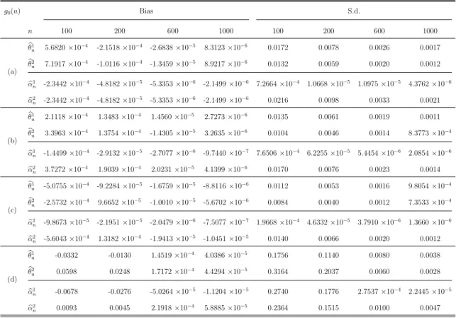
Table 1: Bias and standard deviation for single-index model for case (4.3)
g0(u) Bias S.d. n 100 200 600 1000 100 200 600 1000 (a) b θ1 n 5.6820×10⁻⁴ -2.1518×10⁻⁴ -2.6838×10⁻⁵ 8.3123×10⁻⁶ 0.0172 0.0078 0.0026 0.0017 b θ2 n 7.1917×10⁻⁴ -1.0116×10⁻⁴ -1.3459×10⁻⁵ 8.9217×10⁻⁶ 0.0132 0.0059 0.0020 0.0012 b α1 n -2.3442×10⁻⁴ -4.8182×10⁻⁵ -5.3353×10⁻⁶ -2.1499×10⁻⁶ 7.2664×10⁻⁴ 1.0668×10⁻⁵ 1.0975×10⁻⁵ 4.3762×10⁻⁶ b α2 n -2.3442×10⁻⁴ -4.8182×10⁻⁵ -5.3353×10⁻⁶ -2.1499×10⁻⁶ 0.0216 0.0098 0.0033 0.0021 (b) b θ1 n 2.1118×10− 4 1.3483×10⁻⁴ 1.4560×10⁻⁵ 2.7273×10⁻⁶ 0.0135 0.0061 0.0019 0.0011 b θ2 n 3.3963×10⁻⁴ 1.3754×10⁻⁴ -1.4305×10⁻⁵ 3.2635×10⁻⁶ 0.0104 0.0046 0.0014 8.3773×10⁻⁴ b α1 n -1.4499×10⁻⁴ -2.9132×10⁻⁵ -2.7077×10⁻⁶ -9.7440×10⁻⁷ 7.6506×10⁻⁴ 6.2255×10⁻⁵ 5.4454×10⁻⁶ 2.0854×10⁻⁶ b α2 n 3.7272×10⁻⁴ 1.9039×10⁻⁴ 2.0231×10⁻⁵ 4.1399×10⁻⁶ 0.0170 0.0076 0.0023 0.0014 (c) b θ1 n -5.0755×10− 4 -9.2284×10⁻⁵ -1.6759×10⁻⁵ -8.8116×10⁻⁶ 0.0112 0.0053 0.0016 9.8054×10⁻⁴ b θ2 n -2.5732×10− 4 9.6652×10⁻⁵ -1.0010×10⁻⁵ -5.6702×10⁻⁶ 0.0084 0.0040 0.0012 7.3533×10⁻⁴ b α1 n -9.8673×10⁻⁵ -2.1951×10⁻⁵ -2.0479×10⁻⁶ -7.5077×10⁻⁷ 1.9668×10⁻⁴ 4.6332×10⁻⁵ 3.7910×10⁻⁶ 1.3660×10⁻⁶ b α2 n -5.6043×10⁻⁴ 1.3182×10⁻⁴ -1.9413×10⁻⁵ -1.0451×10⁻⁵ 0.0140 0.0066 0.0020 0.0012 (d) b θ1 n -0.0332 -0.0130 1.4519×10− 4 4.0386×10⁻⁵ 0.1756 0.1140 0.0080 0.0038 b θ2 n 0.0598 0.0248 1.7172×10− 4 4.4294×10⁻⁵ 0.3164 0.2037 0.0060 0.0028 b α1 n -0.0678 -0.0276 -5.0264×10− 5 -1.1204×10⁻⁵ 0.2740 0.1776 2.7537×10⁻⁴ 2.2445×10⁻⁵ b α2 n 0.0093 0.0045 2.1918×10− 4 5.8885×10⁻⁵ 0.2364 0.1515 0.0100 0.0047
The aim of this simulated setting is to illustrate the asymptotic results inTheorem 3.1 and Theorem 3.2. Actually, the rotation technique is not necessary in practice because we will never know the value for the true parameter θ0 and its corresponding rotation
matrix Q. It is only used as a tool to develop the asymptotic theory and can help us better understand the theory.
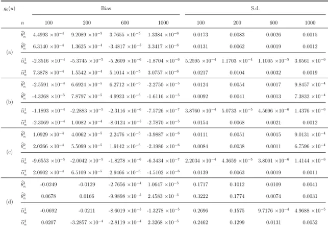
Table 2: Bias and standard deviation for single-index model for case (4.4) g0(u) Bias S.d. n 100 200 600 1000 100 200 600 1000 (a) b θ1 n 4.4993×10⁻⁴ 9.2089×10⁻⁵ 3.7655×10⁻⁵ 1.3384×10⁻⁶ 0.0173 0.0083 0.0026 0.0015 b θ2 n 6.3140×10− 4 1.3625×10⁻⁴ -3.4817×10⁻⁵ 3.3417×10⁻⁶ 0.0131 0.0062 0.0019 0.0012 b α1 n -2.3516×10− 4 -5.3745×10⁻⁵ -5.2609×10⁻⁶ -1.8704×10⁻⁶ 5.2595×10⁻⁴ 1.1703×10⁻⁴ 1.1005×10⁻⁵ 3.6561×10⁻⁶ b α2 n 7.3878×10− 4 1.5542×10⁻⁴ 5.1014×10⁻⁵ 3.0757×10⁻⁶ 0.0217 0.0104 0.0032 0.0019 (b) b θ1 n -2.5591×10⁻⁴ 6.6924×10⁻⁵ 6.2712×10⁻⁵ -2.2750×10⁻⁵ 0.0124 0.0054 0.0017 9.8457×10⁻⁴ b θ2 n -4.3268×10⁻⁵ 7.8797×10⁻⁵ 4.9923×10⁻⁵ -1.6116×10⁻⁵ 0.0092 0.0041 0.0013 7.3832×10⁻⁴ b α1 n -1.1893×10− 4 -2.2883×10⁻⁵ -2.3116×10⁻⁶ -7.5726×10⁻⁷ 3.8760×10⁻⁴ 5.0733×10⁻⁵ 4.5696×10⁻⁶ 1.4376×10⁻⁶ b α2 n -2.3069×10− 4 1.0082×10⁻⁴ -8.0124×10⁻⁵ -2.7870×10⁻⁵ 0.0154 0.0068 0.0021 0.0012 (c) b θ1 n 1.0929×10⁻⁴ 4.0062×10⁻⁵ 2.2476×10⁻⁵ -3.9887×10⁻⁶ 0.0111 0.0051 0.0015 9.0131×10⁻⁴ b θ2 n 2.0266×10⁻⁴ 5.5099×10⁻⁵ 1.9142×10⁻⁵ -2.1986×10⁻⁶ 0.0084 0.0038 0.0011 6.7596×10⁻⁴ b α1 n -9.6553×10⁻⁵ -2.0042×10⁻⁵ -1.8278×10⁻⁶ -6.3434×10⁻⁷ 2.2034×10⁻⁴ 4.3659×10⁻⁵ 3.8001×10⁻⁶ 1.4144×10⁻⁶ b α2 n 2.0902×10⁻⁴ 6.5109×10⁻⁵ 2.9466×10⁻⁵ -4.5102×10⁻⁶ 0.0139 0.0063 0.0019 0.0011 (d) b θ1 n -0.0249 -0.0129 -2.7656×10− 4 1.0647×10⁻⁵ 0.1717 0.1012 0.0109 0.0041 b θ2 n 0.0678 0.0166 -9.9898×10− 5 2.4583×10⁻⁵ 0.3222 0.1774 0.0074 0.0031 b α1 n -0.0692 -0.0211 -8.6019×10⁻⁵ -1.3278×10⁻⁵ 0.2696 0.1575 9.7176×10⁻⁴ 4.9688×10⁻⁵ b α2 n 0.0207 -3.2857×10⁻⁴ -2.8119×10⁻⁴ 2.3268×10⁻⁵ 0.2462 0.1299 0.0131 0.0052
The simulation results of the bias and the standard deviation for θbn = (θb1n,θb2n)>
and αbn = (αb
1
n,αb
2
n)> are summarised in Table 1 and Table 2. We can observe that θbn1
and θbn2 under all four link functions have similar performance. In general, the biases
and standard deviations for θbn decrease with the increase of the sample size n and the
convergence speed is quite fast,5 which verifies the asymptotic theory inTheorem 3.2that
b
θn−θ0 =OP(n−1). In terms of the rotated estimator αbn, both the biases and standard
deviations are approaching zero with the sample size increasing. Moreover, αb1
n converges
at a faster rate than αb2n. This is implied by Theorem 3.1 that αb1n−α10 = OP(n−2) and
b
α2
n−α20 = OP(n−1). It is noteworthy that the biases of αb
1
n are always negative, which
verifies that αb1n is an under-estimator for α10.
Next, we move on to examine the CLT results in Theorem 3.3. The 95% confidence intervals of g0(w) are constructed using the procedure described in Section 4.1. In terms
5 Under the stationary setting, it is well known that
b
θn −θ0 =OP(n−1/2). When n = 1000, the magnitude of the s.d. is about 1000−1/2 = 0.0316; however, under our setting, the s.d. is 10 times smaller than the usual case and is of magnitude around 1000−1= 0.001.
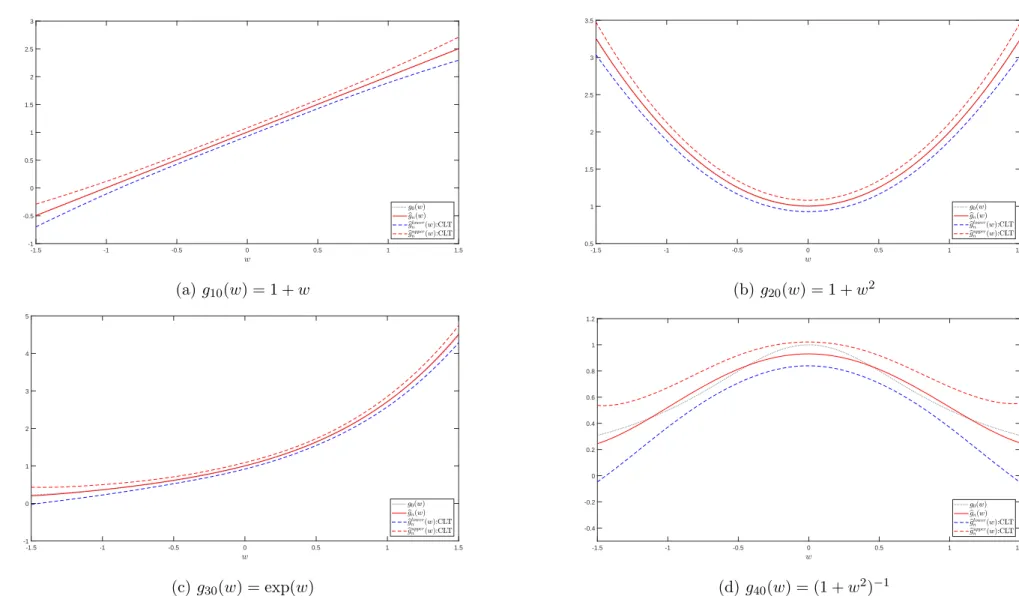
Figure 1: 95% confidence interval for case (4.3) (n=1000) -1.5 -1 -0.5 0 0.5 1 1.5 -1 -0.5 0 0.5 1 1.5 2 2.5 3 (a) g10(w) = 1 +w -1.5 -1 -0.5 0 0.5 1 1.5 0.5 1 1.5 2 2.5 3 3.5 (b)g20(w) = 1 +w2 -1.5 -1 -0.5 0 0.5 1 1.5 -1 0 1 2 3 4 5 (c) g30(w) = exp(w) -1.5 -1 -0.5 0 0.5 1 1.5 -0.4 -0.2 0 0.2 0.4 0.6 0.8 1 1.2 (d)g40(w) = (1 +w2)−1 17
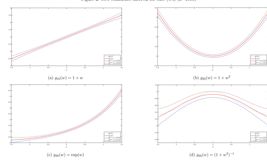
Figure 2: 95% confidence interval for case (4.4) (n=1000) -1.5 -1 -0.5 0 0.5 1 1.5 -1 -0.5 0 0.5 1 1.5 2 2.5 3 (a) g10(w) = 1 +w -1.5 -1 -0.5 0 0.5 1 1.5 0.5 1 1.5 2 2.5 3 3.5 (b)g20(w) = 1 +w2 -1.5 -1 -0.5 0 0.5 1 1.5 0 0.5 1 1.5 2 2.5 3 3.5 4 4.5 5 (c) g30(w) = exp(w) -1.5 -1 -0.5 0 0.5 1 1.5 -0.4 -0.2 0 0.2 0.4 0.6 0.8 1 1.2 (d)g40(w) = (1 +w2)−1 18
of the evaluation pointw, we usen evenly spaced points between -1.5 and 1.5.
We plot the average values of the estimate bgn(w) and the 95% pointwise confidence
interval for each function based on M = 1000 replicated data when n = 1000 inFigure 1 andFigure 2. All the figures show that the 95% pointwise confidence interval constructed from the asymptotic normality covers g0(w) very well and the plot of bgn(w) seems to
coincide with the plot of g0(w), which supports the result in Theorem 3.3.
In addition, we also consider an empirical example in Section 5 below.
5
Empirical study
There is now a large quantity of empirical literature examining the predictability of stock returns using a variety of lagged financial and macroeconomic variables, including dividend-price ratio, earning-price ratio, dividend-payout ratio, book-to-market ratio, interest rates, term spreads and default spreads; see, for example, Lettau and Ludvigson (2001), Cochrane (2011) and Rapach and Zhou (2013). Numerous studies, including those byCampbell and Yogo (2006) andKostakis et al.(2015), have found evidence that many of these predictor variables are highly persistent and are often integrated of order one. If these variables are cointegrated, our semiparametric single-index predictive model can be used to test the predictability of stock returns.6
We extend the univariate linear predictive regression model ofWelch and Goyal(2008), focusing on predictors that can plausibly be modelled as cointegrated. We use their updated monthly and quarterly data over the 1927 to 2017 sample period.7 Their dataset
is one of the most widely used datasets in empirical finance. The dependent variable is the United States (US) equity premium, which is defined as the log return on the S&P 500 index, including dividends minus the log return on a risk-free bill.
Among the 16 financial and macroeconomic variables used byWelch and Goyal(2008) to predict the equity premium, we consider the following four pairs of I(1) variables for which the two variables in each pair are potentially cointegrated: (a) dividend-price ratio
6Recent studies by Koo et al. (2016) and Xu (2017) have found evidence that a subset of these integrated predictors are cointegrated.
Figure 3: Time-series plots of cointegrated predictors 1960 1970 1980 1990 2000 2010 -2 -1.5 -1 -0.5 0 0.5 1
(a) ep and dp (demean)
1960 1970 1980 1990 2000 2010 0 2 4 6 8 10 12 14 16(%) (b) lty and tbl 1960 1970 1980 1990 2000 2010 2 4 6 8 10 12 14 16 18(%)
(c) baa and aaa
1960 1970 1980 1990 2000 2010 -4.6 -4.4 -4.2 -4 -3.8 -3.6 -3.4 -3.2 -3 -2.8 -2.6 (d) dp and dy 20
(dp) and earning-price ratio (ep); (b) three-month T-bill rate (tbl) and long-term yield (lty); (c) BAA- & AAA- rated corporate bond yields; and (d) dp and dividend yield (dy). Welch and Goyal (2008) provided the definitions and sources of these predictors.
For initial illustration, Figure 3 plots the four pairs of cointegrated variables using quarterly data in the sub-period 1952 to 2017, and demonstrated that each pair of vari-ables appeared to be cointegrated. In addition, visual inspection of Figure 1 inCampbell and Yogo (2006) suggests that cointegration is plausible between dp and ep. Fama and French(1989) used the term spread (which is tbl minus lty) and the default spread (which is BAA minus AAA) to predict the equity premium, and, under the assumption that these spreads are stationary, their paper implies that tbl-lty and BAA-AAA are modelled in cointegrating relationships.
A preliminary unit test indicates that every variable has a unit root, while the Engle-Granger Cointegration test suggests the existence of cointegration in each of the four pairs. These tests provide statistical evidence supporting the impression of co-movement behaviour from visually inspecting Figure 3. We now test the hypothesis that the US equity premium is predictable using a linear combination of a pair ofI(1) predictors, via the following semiparametric single-index predictive regression model:
yt=d0+d1ut−1+d2u2t−1+...+dk−1utk−−11+ek,t, (5.1)
with ek,t = γk(ut−1) +et, while the truncation parameter k is determined by the GCV
method described in Section 4.1.8 Under the null hypothesis of no predictability, d
1 = d2 = ... = dk−1 = 0; thus, the model (5.1) reduces to the constant expected equity
premium model. Given that ut−1 ∼ I(0), the no-predictability null hypothesis can be
tested using F-statistic. The OLS coefficient estimates in (5.1) and their conventional standard errors can be obtained in the standard way from a multiple regression of yt on
1, ut−1, u2t−1, ..., ukt−1.
Table 3reports the least-squares estimates of the coefficients in (5.1) and the results of the F-tests under the null hypothesis of no predictability. Numbers in parentheses below the coefficients are t-ratios and below the F-tests are p-values. Panels A and C report
8The use of nonparametric AIC produces identical results. We provide the results of both the GCV and nonparametric AIC methods in the online supplemental material Appendix G.
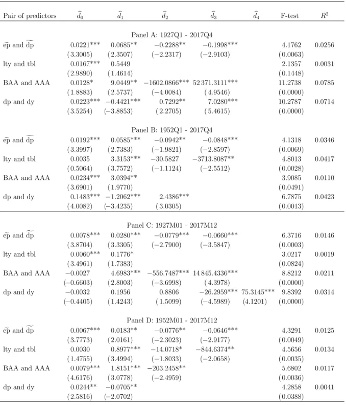
Table 3: Estimates of the single index model parameters and predictive test Pair of predictors db0 db1 db2 db3 db4 F-test R¯2
Panel A: 1927Q1 - 2017Q4 e ep andfdp 0.0221*** 0.0685** −0.2288** −0.1998*** 4.1762 0.0256 ( 3.3005) ( 2.3507) (−2.2317) (−2.9103) ( 0.0063) lty and tbl 0.0167*** 0.5449 2.1357 0.0031 ( 2.9890) ( 1.4614) ( 0.1448)
BAA and AAA 0.0128* 9.0449** −1602.0866*** 52 371.3111*** 11.2738 0.0785 ( 1.8883) ( 2.5737) (−4.0084) ( 4.9546) ( 0.0000) dp and dy 0.0223*** −0.4421*** 0.7292** 7.0280*** 10.2787 0.0714 ( 3.5254) (−3.8853) ( 2.2705) ( 5.4615) ( 0.0000) Panel B: 1952Q1 - 2017Q4 e ep andfdp 0.0192*** 0.0585*** −0.0942** −0.0848*** 4.1318 0.0346 ( 3.3997) ( 2.7383) (−1.9821) (−2.8597) ( 0.0069) lty and tbl 0.0035 3.3153*** −30.5827 −3713.8087** 4.8013 0.0417 ( 0.5064) ( 3.7572) (−1.1124) (−2.5512) ( 0.0028)
BAA and AAA 0.0234*** 3.0394** 3.9085 0.0110
( 3.6901) ( 1.9770) ( 0.0491) dp and dy 0.1483*** −1.2062*** 2.4386*** 6.7875 0.0423 ( 4.0082) (−3.4235) ( 3.0305) ( 0.0013) Panel C: 1927M01 - 2017M12 e ep andfdp 0.0078*** 0.0280*** −0.0779*** −0.0660*** 6.3716 0.0146 ( 3.8704) ( 3.3305) (−2.7900) (−3.5847) ( 0.0003) lty and tbl 0.0060*** 0.1776* 3.0217 0.0019 ( 3.4961) ( 1.7383) ( 0.0824)
BAA and AAA −0.0027 4.6983*** −556.7487*** 14 845.4336*** 8.8212 0.0211 (−0.6603) ( 2.8003) (−3.6998) ( 4.3978) ( 0.0000) dp and dy −0.0032 0.1956 0.8806 −26.2959*** 75.3145*** 9.8392 0.0314 (−0.4405) ( 1.4243) ( 1.5099) (−4.5989) (4.1201) ( 0.0000) Panel D: 1952M01 - 2017M12 e ep andfdp 0.0067*** 0.0183** −0.0776** −0.0646*** 4.3291 0.0125 ( 3.7773) ( 2.0161) (−2.3023) (−2.9177) ( 0.0049) lty and tbl 0.0030 0.8977*** −14.0718* −844.6374** 4.5656 0.0134 ( 1.4755) ( 3.4994) (−1.8033) (−2.0658) ( 0.0035)
BAA and AAA 0.0079*** 1.8151*** −203.2458** 5.6802 0.0117 ( 4.6176) ( 3.0778) (−2.4959) ( 0.0036)
dp and dy 0.0244** −0.0705** 4.2858 0.0041
( 2.5816) (−2.0702) ( 0.0388)
Notes: This table reports ordinary least squares estimates of the parameters in (5.1). The dependent variable ytis the US equity premium, while the lagged regressors,x1,t−1andx2,t−1, are the cointegrated predictors. Four pairs of cointegrated predictors are considered, as follows: (i) ep (earning-price ratio) and dp (dividend-price ratio), (ii) tbl (T-bill rate) and lty (long-term yield), (iii) BAA and AAA (-rated corporate bond yields), and (iv) dp and dy (dividend yield). We use the GCV method to select the truncation parameterk.The F-tests are computed under the null hypothesis of no predictability—that is,H0:d1=d2=...=dk= 0. The number in
parenthesis below each estimate ist-ratio and below eachF-test isp-value. Panels A and B (C and D) report estimation results for the quarterly (monthly) data. *,**,*** indicate significance at the 10%, 5% and 1% levels, respectively.
the results for the whole sample period of 1927 to 2017, based on quarterly and monthly data, respectively. FollowingKostakis et al.(2015), we also consider the post-1952 period because the interest rate variables are expected to be linked together after the Federal Reserve abandoned the interest rate pegging policy in 1951. Moreover, Campbell and Yogo (2006) and Kostakis et al. (2015) reported weak or no evidence of stock return predictability in the post-1952 period. Our results for this sub-period are reported in Panels B (quarterly data) and D (monthly data).
In Table 3, using the F-tests, we reject the null hypothesis of no predictability at the 5% level in both the full sample and the post-1952 sample for all four pairs at quarterly and monthly frequencies, with one exception. The pair of lty and tbl is not a significant predictor of equity premium at quarterly and monthly frequencies in the full sample, yet is a significant predictor in the post-1952 period. This result supports the view that the term-structure variables are closely linked together after 1952, yet not before.
While numerous studies (such as Campbell and Yogo,2006 andKostakis et al.,2015) found no or weak evidence of predictability in the post-1952 period using a univariate or multivariate framework, we do find strong evidence using bivariate cointegrated predictors in this sub-period.
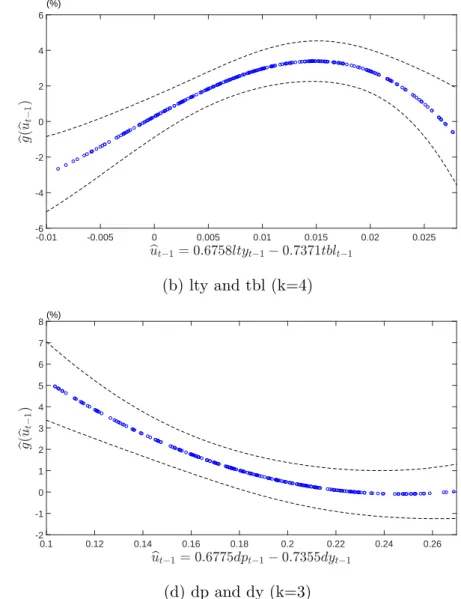
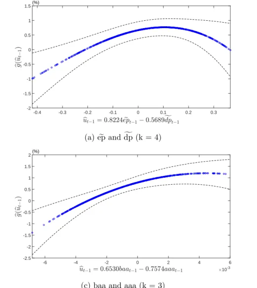
Moreover, the results in Table 3 provide ample evidence in favour of nonlinear pre-dictability of stock returns, since the coefficients on the highest power in the polynomial regression (5.1) are statistically significant at conventional levels. To illustrate the approx-imate form of nonlinearity, Figure 4 plots predicted value of equity premium, bgn(but−1),
againstbut−1 =θb1x1,t−1+θb2x2,t−1, along with the 90% pointwise confidence intervals using
the post-1952 quarterly data. The confidence intervals are obtained using the procedure described in Section 4.1. The corresponding plots for the monthly data are given in Figure 5.
Figure 4 and Figure 5 indicate that the pair of lty and tbl and pair of ep and dp exhibit a hump-shaped relationship between bgn(ubt−1) and ubt−1 at both quarterly and
monthly frequencies. This empirical finding of nonlinear predictability using these two pairs of cointegrated predictors highlights a useful feature of our proposed semiparametric single-index predictive model. Using quarterly lty and tbl as an illustration, Figure 4 shows that the predicted value of equity premium peaks at around but−1 = 0.6758ltyt−1−
Figure 4: Estimated link function bg(but−1) at quarterly frequency -0.4 -0.3 -0.2 -0.1 0 0.1 0.2 0.3 0.4 0.5 -4 -3 -2 -1 0 1 2 3 4(%) (a) ep ande dp (k = 4)f -0.01 -0.005 0 0.005 0.01 0.015 0.02 0.025 -6 -4 -2 0 2 4 6 (%) (b) lty and tbl (k=4) -8 -7 -6 -5 -4 -3 -2 -1 0 1 2 3 10-3 -2 -1 0 1 2 3 4 5 (%)
(c) baa and aaa (k = 2)
0.1 0.12 0.14 0.16 0.18 0.2 0.22 0.24 0.26 -2 -1 0 1 2 3 4 5 6 7 8(%) (d) dp and dy (k=3) 24
Figure 5: Estimated link functionbg(ubt−1) at monthly frequency -0.4 -0.3 -0.2 -0.1 0 0.1 0.2 0.3 -2 -1.5 -1 -0.5 0 0.5 1 1.5(%) (a) ep ande dp (k = 4)f -0.015 -0.01 -0.005 0 0.005 0.01 0.015 0.02 0.025 -2 -1.5 -1 -0.5 0 0.5 1 1.5(%) (b) lty and tbl (k=4) -6 -4 -2 0 2 4 6 10-3 -2.5 -2 -1.5 -1 -0.5 0 0.5 1 1.5 2(%)
(c) baa and aaa (k = 3)
0.2 0.25 0.3 0.35 0.4 -1.5 -1 -0.5 0 0.5 1 1.5 2(%) (d) dp and dy (k=2)
Notes: This figure plots the estimated link function of each pair of comoving predictors. The dashed line shows the approximate 90%
0.7371tblt−1 = 0.015. In contrast, there is a small or negligible amount of nonlinear
predictability of equity premium using the pair of BAA and AAA and the pair of dp and dy, at quarterly and monthly frequencies.
6
Conclusion
This paper has proposed estimation procedures for the single-index predictive regres-sion model when the nonstationary predictors exhibit co-movement behaviour. We have studied the two types of super-consistency rates for the estimator of the single-index pa-rameter θ0 along two orthogonal directions in a new coordinate system, as well as their
corresponding asymptotic distributions. This paper has also established the asymptotic normality of the plug-in estimator of the unknown link function. In addition, through Monte-Carlo simulations, we have evaluated the finite-sample properties of αbn, θbn, as
well as bgn. Further, we have applied the proposed model in the context of stock return
predictability, and found nonlinear predictability of the equity premium using four pairs of comoving predictors.
Appendix A
Discussion on the assumptions
For Assumption 1.1 (a), similar arguments are widely used in the literature for nonstationary models, such as byPark and Phillips(2000,2001), and theσ-field sequenceFn,t−1 can be taken
as Fn,t−1 = σ(x1,· · ·, xn−1;e1,· · ·, et−1). For Assumption 1.2 (a)−(b), suppose that xt is a
d-dimensional integrated process, which is generated by a linear processvtwith i.i.d. sequence {j,−∞ < j < ∞} in Assumption 1.1 (b) as building blocks. Assumption 1.2 (c) assumes a cointegration structure for xt, and more details of cointegration structure have been discussed by Granger and Weiss (1983) andEngle and Granger (1987). Assumption 1.2 (c) also implies that there exists only one cointegration equation among xt. This is an important assumption to develop the asymptotic theory for θbn−θ0 using the rotation technique because we need to ensure that x2t is a pure (d−1)-dimensional nonstationary process. Assumption 1.2 (d) is our main assumption, in which we considerθ0>xtto be stationary inside the unknown link function, even though xt is ad-dimensional integrated process. We also impose some restrictions on the probability density function ofut=θ>0xtto exclude heavy-tailed distributions, and subsequently
can control the potentially unbounded support and unbounded function smoothly.
Assumption 1.3 assumes the consistency for (θbn, b
gn) directly. The consistency is established with respect to the norm k.k2 defined in (2.6). This assumption implies that θbn →P θ0 and kbgn−g0kL2 →P 0, respectively. Letδ >0 and define Θδ×Gδ={
(θ, g)−(θ0, g0)
2 ≥δ} ⊂Θ× G. This assumption can be replaced by the conditionPn
t=1
g(θ>xt−1)−g0(θ0>xt−1)
2
→P ∞
uniformly in (θ, g)∈Θδ×Gδ. To prove the consistency under this condition, define:
An= n X t=1 g(θ>xt−1)−g0(θ0>xt−1) 2 , Bn= n X t=1 g(θ>xt−1)−g0(θ0>xt−1) et, Dn= n X t=1 yt−g(θ>xt−1) 2 − n X t=1 yt−g0(θ>0xt−1) 2 .
Then we can show that:
E h A−n1/2Bn i2 =E n X t=1 g(θ>xt−1)−g0(θ>0xt−1) 2 −1/2 n X t=1 g(θ>xt−1)−g0(θ0>xt−1) et 2 =E n X t=1 g(θ>xt−1)−g0(θ>0xt−1) 2 −1 n X t=1 g(θ>xt−1)−g0(θ>0xt−1) 2 Ehe2t|Fn,t−1 i =σ 2.
Therefore, A−n1/2Bn=OP(1) uniformly in (θ, g)∈Θδ×Gδ. Then, we have:
Dn=An(1−A−n1Bn) =An(1 +oP(1))→P ∞,
uniformly in (θ, g)∈Θδ×Gδ. Given that Θδ×Gδ is compact, we may easily deduce that: inf
(θ,g)∈Θδ×Gδ
Dn→P ∞.
This condition is sufficient to ensure the consistency, as shown in earlier work by Wu (1981): for any δ >0, lim infn→∞infk(θ,g)−(θ0,g0)k2≥δDn>0 in probability.
To verity the assumption thatPn t=1
g(θ>xt−1)−g0(θ>0xt−1)
2
→P ∞uniformly in (θ, g)∈ Θδ×Gδ, we consider four cases:
(1) Given the point (θ0, g) ∈ Θδ×Gδ, by Weak Law of Large Numbers (WLLN), we can show that 1 n n X t=1 g(θ0>xt−1)−g0(θ0>xt−1) 2 →P E g(x11)−g0(x11) 2
uniformly in (θ0, g)∈Θδ×Gδ andE
g(x11)−g0(x11)
2
>0 is implied bykg−g0k2L2 > δ2 >0.
Then we can obtain thatPn t=1
g(θ0>xt−1)−g0(θ0>xt−1)
2
→P ∞uniformly in (θ0, g)∈Θδ×Gδ. (2) Given the point (θ, g0)∈Θδ×Gδ, suppose thatg0 isH-regular such that:
g0(ηx) =κ(η)H(x) +ξ(η;x), ξ(η;x)
≤a(η)P(x),
whereH(x) and P(x) are both locally integrable, lim supη→∞a(η)/κ(η) = 0 and κ( √
n)→ ∞
asn→ ∞.
According to (19) in Phillips and Solo(1992), we have:
sup r 1 n1/2 bnrc X t=1 θ>xt−1−θ>φ(1) 1 n1/2 bnrc X t=1 t−1 →P 0.
We further suppose that, for all m >0,R|r|≤mH(r)2dr >0. Then we can show that:
1 nκ( √ n)2 n X t=1 g0(θ>xt−1)−g0(θ0>xt−1) 2 →P Z 1 0 H(Vθ(r))2dr
uniformly in (θ, g0) ∈ Θδ ×Gδ, where Vθ is Brownian motion of dimension 1 with variance ΣVθ =θ
>φ(1)Σ
φ(1)>θ. Define a scaled local time L of Vθ by L(t, s) = 1/ΣVθLVθ(t, s), where LVθ is the local time of Brownian motionVθ(r). By the occupation formula for Brownian motion:
Z 1 0 H(Vθ(r))2dr= Z H(s)2L(1, s)ds≥ Z |s|≤m H(s)2L(1, s)ds >0 a.s..
Then we can obtain thatPn t=1 g0(θ>xt−1)−g0(θ>0xt−1) 2 →P ∞ uniformly in (θ, g0)∈Θδ× Gδ.
(3) Given the point (θ, g0)∈Θδ×Gδ, and suppose that g0 is I-regular, we can show that:
1 n n X t=1 g0(θ>xt−1)−g0(θ0>xt−1) 2 →P E g0(x11) 2 >0,
uniformly in (θ, g0)∈Θδ×Gδ. Then we can obtain thatPnt=1
g0(θ>xt−1)−g0(θ0>xt−1)
2 →P ∞ uniformly in (θ, g0)∈Θδ×Gδ.
(4) Given the point (θ, g)∈Θδ×Gδ, following the same ideas in cases (2) and (3), we can show that Pn t=1 g(θ>0xt−1)−g0(θ>xt−1) 2 →P ∞ uniformly in (θ, g) ∈ Θδ×Gδ when g is
H-regular andI-regular, respectively. For more details aboutH-regular andI-regular, we refer toPark and Phillips (2001).
Assumption 1.4 assumes a high degree of smoothness for the unknown link function g0(w),
choose the truncation parameter, it must satisfy some conditions in Assumption 1.5 to ensure that the estimators θbn and
b
gn converge with a certain rate. In addition, we also consider the identification condition that inf
c∈R
E
h
g0(θ0>x1)−c
i2
> 0 in Assumption 1.6 (a). If there exists
c ∈ R such that Ehg0(θ>0x1)−c
i2
= 0, then θ0 will be unidentifiable. Assumption 1.6 (b)
is standard in the literature (Newey, 1997). Suppose that ut = θ>0xt ∼ iiN(0,1), we have
EhHk(u1)Hk(u1)>
i
= (2π)−1/2Ik, where Ik is a k-dimensional identity matrix. Then all the eigenvalues of E
h
Hk(u1)Hk(u1)>
i
are (2π)−1/2, and hence they are bounded away from zero uniformly in k≥1.
InAssumption 1.7 (a), we require the fourth moment ofg0(θ>0xt−1) to exist, and many
func-tional forms forg0(.) together withAssumption 1.2 (d) can satisfy this condition. Supposeg0(.)
to be polynomials (e.g. g0(w) = 1+w2), exponential functions (e.g. g0(w) = exp(w)) or bounded
functions (e.g. g0(w) = (1 +w2)−1), and it is easy to see that g0(w)∈L2(R.exp(−w2/2)) and
g0(w)
2
∈ L2(R.exp(−w2/2)). Then, simple algebra can show that Assumption 1.7 (a) is satisfied. Assumption 1.7 (b) can be replaced by a stronger version of Assumption 1.2 (d), as follows:
• Suppose that ut = θ>0xt is a strictly stationary time series and has probability density functionρ(u) such that exp(u2)ρ(u)<∞ uniformly inu.
Follow the truth thatHi(u)
×exp(−u2/4) being bounded uniformly, we are able to show that 1 n k−1 X i=0 k−1 X j=0 E Hi(u1)Hj(u1) 2 = 1 n k−1 X i=0 k−1 X j=0 Z Hi2(u)Hj2(u)ρ(u)du =1 n k−1 X i=0 k−1 X j=0 Z
Hi2(u) exp(−u2/2)Hj2(u) exp(−u2/2) exp(u2)ρ(u)du
≤O(1)1 n k−1 X i=0 k−1 X j=0 Z Hj2(u) exp(−u2/2)du.=O(n−1k2) =o(1).
Alternatively, we can assumeE
Hi(u1)
4
is uniformly bounded for 1≤i≤k−1, and then
Assumption 1.7 (b) can be easily verified.
Assumption 1.7 (c) and (d) can be replaced by a condition on the density function ofjand a condition on the coefficients of the linear process forvt. According to the Beveridge and Nelson (BN) decomposition Beveridge and Nelson,1981forxt, we can write x1t=θ0>xt=P∞i=0dit−i (more details can be found in the proof of Lemma 3 in Appendix D). Suppose that: (1) the innovations {j,−∞ < j <∞} have density p(x) satisfying
R
p(x)−p(x+y)
≤ C|y| where 0< C <∞; and (2) limj→∞djjλ exists withλ >11/4. Then, using the Corollary 4 inWithers
(1981), we can show that the linear processx1tis aα-mixing process with mixing coefficientα(τ), such thatα(τ) =O(τ−1/2) and hence 1nPn−1
τ=1α(τ)ν/(4+ν) =O(n−1/2) for someν >0. In
addi-tion, we also need to assume thatE
g (1) 0 (θ>0x1) 4+ν <∞and max0≤i≤k−1E Hi(θ > 0x1) 4+ν <∞
for the sameν defined before.
Then for Assumption 1.7 (c), we can show that: 1 n2 n X t=2 t−1 X s=1 Cov g(1)0 (θ0>xt−1) 2 ,g0(1)(θ>0xs−1) 2 = 1 n2 n X t=2 t−1 X s=1 Cov g(1)0 (x1t−1) 2 ,g(1)0 (x1s−1) 2 =1 n n−1 X τ=1 1− τ n Cov g0(1)(x11) 2 ,g(1)0 (x1,1+τ) 2 ≤cα 1 n n−1 X τ=1 1− τ n α(τ)ν/(4+ν) E h g(1)0 (x11) i(4+ν)4/(4+ν) =O(1)1 n n−1 X τ=1 1− τ n α(τ)ν/(4+ν)=O(n−1/2) =o(1), wherecα = 2(4+2ν)/(4+ν)×(4 +v)/v.
Similarly, in terms ofAssumption 1.7 (d), we have:
1 n2 k−1 X i=0 k−1 X j=0 n X t=2 t−1 X s=1 CovHi(θ0>xt−1)Hj(θ0>xt−1), Hi(θ0>xs−1)Hj(θ>0xs−1) = 1 n2 k−1 X i=0 k−1 X j=0 n X t=2 t−1 X s=1 Cov Hi(x1t−1)Hj(x1t−1), Hi(x1s−1)Hj(x1s−1) =1 n k−1 X i=0 k−1 X j=0 n−1 X τ=1 1−τ n Cov Hi(x11)Hj(x11), Hi(x1,1+τ)Hj(x1,1+τ) ≤cα 1 n k−1 X i=0 k−1 X j=0 n−1 X τ=1 1−τ n α(τ)ν/(4+ν)E Hi(x11)Hj(x11) (4+ν)/24/(4+ν) ≤cα 1 n k−1 X i=0 k−1 X j=0 n−1 X τ=1 1−τ n α(τ)ν/(4+ν)EHi(x11) 4+ν EHj(x11) 4+ν2/(4+ν) =O(1)1 n k−1 X i=0 k−1 X j=0 n−1 X τ=1 1−τ n α(τ)ν/(4+ν)=O(n−1/2k2) =o(1).
Appendix B
Proofs of the theorems
According to Lemma 9inAppendix C, we have as n→ ∞ P1>Dn(αbn−α0)→D σr −1/2 0 W(1). Since P1 = p1,1 ··· p1,d−1 .. . ... ... pd,1 ··· pd,d−1 !
withpi+1,i= 1 for 1≤i≤d−1 and others equal zero, simple algebra shows that
n(αb2n−α20)→D ξ.
In addition, notice that
b
θn>θ0−1 =(θbn−θ0)>θ0 = (θbn−θ0)>(θ0−θbn+θbn) =−kθbn−θ0k2−(θbn>θ0−1).
Therefore, θbn>θ0−1 =−1
2kθbn−θ0k 2.
Consider the orthogonal expansion that kθbn−θ0k2 =kQ>2(θbn−θ0)k2+kθ0>(θbn−θ0)k2, we can obtain n2(αb1n−α10) =n2θ0>(bθn−θ0) =− 1 1 +θ>0θbn knQ>2(θbn−θ0)k2 =−1 2knQ > 2(θbn−θ0)k2(1 +oP(1))→D − 1 2kξk 2. Proof of Theorem 3.2:
Since θbn is the composite of b α1n and αb2n, we have n(bθn−θ0) =Qn( b αn−α0) =Qn b α1n−1 b α2n =(θ0, Q2) 0 nαb2n +oP(1) =Q2nαb 2 n+oP(1) →D MN(0, σ2Q2r−01Q > 2). Proof of Theorem 3.3:
We first show the consistency of Hbx and σb2. Hbx →P Hx follows from Lemma 5 in
Ap-pendix C directly. For bσ2, note that
b σ2 = 1 n n X t=1 h yt−bgn(θb > nxt−1) i2
=1 n n X t=1 et+g0(x1t−1)−bgn(ηbt−1) 2 =1 n n X t=1 e2t+ 1 n n X t=1 g0(x1t−1)−bgn(ηbt−1) 2 + 2 n n X t=1 et g0(x1t−1)−bgn(ηbt−1) :=A1+A2+ 2A3. It is obvious that A1 →P σ2.
Given any >0, define for any function f(x)∈L2(R,exp(−x2/2)),
fsup (x) = sup |α−1|< sup |b|< f(ax+b) .
The discussion of its properties can be found in the proof of Lemma 5inAppendix D. For A2, write A2 = 1 n n X t=1 g0(x1t−1)−bgn(bηt−1) 2 =1 n n X t=1 g0(x1t−1)−g0(ηbt−1) +gk(ηbt−1)−bgn(bηt−1) +γk(ηbt−1)−γk(x1t−1) +γk(x1t−1) 2 ≤O(1)1 n n X t=1 g0(x1t−1)−g0(ηbt−1) 2 +O(1)1 n n X t=1 gk(ηbt−1)−bgn(bηt−1) 2 +O(1)1 n n X t=1 γk(ηbt−1)−γk(x1t−1) 2 +O(1)1 n n X t=1 γk(x1t−1) 2 ≤O(1) bα 1 n−α10 2 1 n n X t=1 g0(1) sup(x1t−1)x1t−1 2 (1 +oP(1)) +O(1) bα 2 n−α20 2 1 n n X t=1 g0(1) sup(x1t−1)x2t−1 2 (1 +oP(1)) +O(1)C¯k(αbn)−C0,k 2 1 n n X t=1 k−1 X i=0 h (Hi)sup(x1t−1) i2 (1 +oP(1)) +O(1) bα 1 n−α10 2 1 n n X t=1 γk(1) sup(x1t−1)x1t−1 2 (1 +oP(1)) +O(1) bα 2 n−α20 2 1 n n X t=1 γk(1) sup(x1t−1)x2t−1 2 (1 +oP(1)) +O(1)1 n n X t=1 γk(x1t−1) 2 :=O(1)A2,1+· · ·+O(1)A2,6.
Similar to the proof of (E.3) in online Appendix E, we can show that kC¯k(αbn)−C0,kk =
OP(n−1/2k1/2) +oP(k−r/2). Then, we can obtain that
A2,3 =OP(n−1k2) +oP(k−(r−1)), A2,5 =oP(n−4k−(r−2)),
A2,6 =oP(n−1k−(r−1)), A2,7 =oP(k−r),
and hence we have shown thatA2 =oP(1).
For the proof of the normality, in view of the consistency of σb and Hbx, we show the result with the replacement of σ and Hx. Let Zb=Z(θbn) =Z(αbn) and write
b gn(w)−g0(w) +γk(w) =Hk(w)> ¯ Ck(θbn)−C0,k =Hk(w)>Zb>Zb −1 b Z>(γ+e) +Hk(w)>Zb>Zb −1 b Z>Z−Zb C0,k =1 nHk(w) >H−1 x Zb>e(1 +oP(1)) + 1 n1/2Hk(w) >H−1/2 x Z>Z −1/2 b Z>γ(1 +oP(1)) +1 nHk(w) >H−1 x Zb> Z−Zb C0,k(1 +oP(1)) =1 nHk(w) >H−1 x Ze(1 +oP(1)) + 1 nHk(w) >H−1 x b Z−Z > e(1 +oP(1)) + 1 n1/2Hk(w) >H−1/2 x Z>Z−1/2Z>γ(1 +oP(1)) + 1 nHk(w) >H−1 x b Z−Z>γ(1 +oP(1)) +1 nHk(w) >H−1 x Z > Z−Zb C0,k(1 +oP(1)) +1 nHk(w) >H−1 x b Z−Z>Z−Zb C0,k(1 +oP(1)) Then it follows that
√ nΣ−1(w) bgn(w)−g0(w) +γk(w) =n−1/2σ−1Hk(w)>H−1 x Hk(w) −1/2 Hk(w)>H−1 x Z >e(1 +o P(1)) +n−1/2σ−1Hk(w)>Hx−1Hk(w) −1/2 Hk(w)>H−x1Zb−Z > e(1 +oP(1)) +σ−1 Hk(w)>H−x1Hk(w) −1/2 Hk(w)>Hx−1/2 Z>Z −1/2 Z>γ(1 +oP(1)) +n−1/2σ−1Hk(w)>H−1 x Hk(w) −1/2 Hk(w)>H−1 x b Z−Z>γ(1 +oP(1)) +n−1/2σ−1Hk(w)>Hx−1Hk(w) −1/2 Hk(w)>Hx−1Z>Z−Zb C0,k(1 +oP(1)) +n−1/2σ−1 Hk(w)>Hx−1Hk(w) −1/2 Hk(w)>H−x1 b Z−Z > Z−Zb C0,k(1 +oP(1)) =F1(1 +oP(1)) +· · ·+F6(1 +oP(1))
By Assumption 1.1, F1 is a martingale array and we shall use Corollary 3.1 of Hall and Heyde(1980) to show that F1 →D N(0,1).
The conditional variance process is given by 1 nσ −2H k(w)>H−x1Hk(w) −1Xn t=1 Hk(w)>Hx−1Hk(x1t−1) 2 E h e2t|Fn,t−1 i