A Multiscale Pyramid Transform for Graph Signals
David I Shuman, Mohammad Javad Faraji, and Pierre Vandergheynst
Abstract—Multiscale transforms designed to process analog and discrete-time signals and images cannot be directly applied to analyze high-dimensional data residing on the vertices of a weighted graph, as they do not capture the intrinsic geometric structure of the underlying graph data domain. In this paper, we adapt the Laplacian pyramid transform for signals on Euclidean domains so that it can be used to analyze high-dimensional data residing on the vertices of a weighted graph. Our approach is to study existing methods and develop new methods for the four fundamental operations of graph downsampling, graph reduction, and filtering and interpolation of signals on graphs. Equipped with appropriate notions of these operations, we leverage the basic multiscale constructs and intuitions from classical signal processing to generate a transform that yields both a multiresolution of graphs and an associated multiresolution of a graph signal on the underlying sequence of graphs.
Index Terms—Signal processing on graphs, multiresolution, spectral graph theory, graph downsampling, Kron reduction, spectral sparsification, Laplacian pyramid, interpolation
I. INTRODUCTION
Multiscale transform methods can reveal structural informa-tion about signals, such as singularities or irregular structural patterns, at different resolution levels. At the same time, via coarse-to-fine analysis, they provide a way to reduce the complexity and dimensionality of many signal processing tasks, often resulting in fast algorithms. However, multiscale transforms such as wavelets and filter banks designed to process analog and discrete-time signals and images cannot be directly applied to analyze high-dimensional data residing on the vertices of a weighted graph, as they do not capture the intrinsic geometric structure of the underlying graph data domain (see [2] for an overview of the main challenges of this emerging field of signal processing on graphs).
To address this issue, classical wavelets have recently been generalized to the graph setting in a number of different ways. Reference [2] contains a more thorough review of these graph wavelet constructions, which include, e.g., spatially-designed graph wavelets [3], diffusion wavelets [4], spectral graph wavelets [5], lifting based wavelets [6], [7] critically sampled This work was supported in part by FET-Open grant number 255931 UNLocX.
Part of this work appeared in the master’s thesis [1] and was presented at the Duke Workshop on Sensing and Analysis of High-Dimensional Data in July 2011. Slides and video are available at http://sahd.pratt.duke.edu/2011 files/Videos and Slides.html
David I Shuman is with the Department of Mathematics, Statistics, and Computer Science, Macalester College, St. Paul, MN 55105, USA (email: [email protected]). Mohammad Javad Faraji is with the Compu-tational Neuroscience Laboratory (LCN), Ecole Polytechnique F´ed´erale de Lausanne (EPFL), School of Computer and Communication Sciences and Brain Mind Institute, School of Life Sciences, CH-1015 Lausanne, Switzer-land (email: [email protected]). Pierre Vandergheynst is with the Signal Processing Laboratory (LTS2), Ecole Polytechnique F´ed´erale de Lausanne (EPFL), Institue of Electrical Engineering, CH-1015 Lausanne, Switzerland (email: [email protected]).
two-channel wavelet filter banks [8], critically-sampled spline wavelet filter banks [9], and multiscale wavelets on balanced trees [10]. Multiresolutions of graphs also have a long history in computational science problems including graph cluster-ing, numerical solvers for linear systems of equations (often arising from discretized differential equations), combinatorial optimization problems, and computational geometry (see, e.g., [11]-[14] and references therein). We discuss some of the related work from these fields in Sections III-E and IV-E.
In this paper, we present a modular framework for adapting Burt and Adelson’s Laplacian pyramid transform [15] to the graph setting. Our main contributions are to (1) survey differ-ent methods for and desirable properties of the four fundamen-tal graph signal processing operations of graph downsampling, graph reduction, generalized filtering, and interpolation of graph signals (Sections III-V); (2) present new graph down-sampling and reduction methods, including downdown-sampling based on the polarity of the largest Laplacian eigenvector and Kron reduction followed by spectral sparsification; and (3) leverage these fundamental operations to construct a new multiscale pyramid transform that yields both a multiresolution of a graph and a multi-scale analysis of a signal residing on that graph (Section VI). We also discuss some implementation approximations and open issues in Section VII, as it is important that the computational complexity of the resulting multiscale transform scales well with the number of vertices and edges in the underlying graph.
II. SPECTRALGRAPHTHEORYNOTATION
We consider connected, loopless (no edge connecting a vertex to itself), undirected, weighted graphs. We represent such a graph by the tripletG={V,E, w}, whereV is a set of
N vertices,E is a set of edges, andw:E →R+ is a weight
function that assigns a non-negative weight to each edge. An equivalent representation is G = {V,E,W}, where W is a
N×N weighted adjacency matrix with nonnegative entries
Wij =
(
w(e), ife∈ E connects verticesi andj 0, if no edge connects verticesiandj .
In unweighted graphs, the entries of the adjacency matrixW are ones and zeros, with a one corresponding to an edge between two vertices and a zero corresponding to no edge. The degree matrixDis a diagonal matrix with anithdiagonal element Dii = di = Pj∈NiWij, where Ni is the set of
vertex i’s neighbors in G. Its maximum element is dmax :=
maxi∈V{di}. We denote the combinatorial graph Laplacian
by L := D−W, the normalized graph Laplacian by L˜ :=
D−12LD− 1
2, and their respective eigenvalue and eigenvector
pairs by {(λ`,u`)}`=0,1,...,N−1 and {(˜λ`,u˜`)}`=0,1,...,N−1. ThenUandU˜ are the matrices whose columns are equal to the
eigenvectors ofLandL˜, respectively. We assume without loss of generality that the eigenvalues are monotonically ordered so that 0 = λ0 < λ1 ≤ λ2 ≤ . . . ≤ λN−1, and we denote the maximum eigenvalues and associated eigenvectors by
λmax=λN−1 andumax=uN−1. The maximum eigenvalue
λmax is said to be simpleifλN−1> λN−2. III. GRAPHDOWNSAMPLING
Two key components of multiscale transforms for discrete-time signals are downsampling and upsampling.1 To
down-sample a discrete-time down-sample by a factor of two, we remove every other component of the signal. To extend many ideas from classical signal processing to the graph setting, we need to define a notion of downsampling for signals on graphs. Yet, it is not at all obvious what it means to remove every other component of a signal f ∈RN defined on the vertices
of a graph. In this section, we outline desired properties of a downsampling operator for graphs, and then go on to suggest one particular downsampling method.
Let D : G = {V,E,W} → 2V be a graph downsampling
operator that maps a weighted, undirected graph to a subset of vertices V1 to keep. The complement V1c := V\V1 =
{v∈ V:v /∈ V1} is the set of vertices that D removes from
V. Ideally, we would like the graph downsampling operatorD
to have the following properties:
(D1) It removes approximately half of the vertices of the graph (or, equivalently, approximately half of the com-ponents of a signal on the vertices of the graph); i.e.,
|D(G)|=|V1| ≈ |V|2 .
(D2) The set of removed vertices are not connected with edges of high weight, and the set of kept vertices are not connected with edges of high weight; i.e., if i, j∈ V1, thenWij is low, and ifi, j∈ Vc
1, thenWij is low. (D3) It has a computationally efficient implementation.
A. Vertex Selection Using the Largest Eigenvector of the Graph Laplacian
The method we suggest to use for graph downsampling is to select the vertices to keep based on the polarity of the components of the largest eigenvector; namely, let
V1=V+:={i∈ V :umax(i)≥0}. (1) We refer to this method as the largest eigenvector vertex selection method. A few remarks are in order regarding this choice of downsampling operator. First, the polarity of the largest eigenvector splits the graph into two components. In this paper, we choose to keep the vertices in V+, and eliminate the vertices in V− := {i∈ V :umax(i)<0}, but we could just as easily do the reverse, or keep the vertices in Vbig := arg maxV1∈{V+,V−}|V1|, for example. Second, for
some graphs such as the complete graph, λmax is a repeated eigenvalue, so the polarity of umax is not uniquely defined. In this case, we arbitrarily choose an eigenvector from the 1We focus here on downsampling, as we are only interested in upsampling previously downsampled graphs. As long as we track the positions of the removed components of the signal, it is straightforward to upsample by inserting zeros back into those components of the signal.
eigenspace. Third, we could just as easily base the vertex selection on the polarity of the normalized graph Laplacian eigenvector, u˜max associated with the largest eigenvalue,
˜
λmax. In some cases, such as the bipartite graphs discussed next, doing so yields exactly the same selection of vertices as downsampling based on the largest non-normalized graph Laplacian eigenvector; however, this is not true in general.
In the following sections, we motivate the use of the largest eigenvector of the graph Laplacian from two different perspec-tives - first from a more intuitive view as a generalization of downsampling techniques for special types of graphs, and then from a more theoretical point of view by connecting the vertex selection problem to graph coloring, spectral clustering, and nodal domain theory.
B. Special Case: Bipartite Graphs
There is one situation in which there exists a fairly clear notion of removing every other component of a graph signal – when the underlying graph is bipartite. A graph G = {V,E,W} is bipartite if the set of vertices V can be par-titioned into two subsetsV1 andV1c so that every edgee∈ E links one vertex in V1 with one vertex in V1c. In this case, it is natural to downsample by keeping all of the vertices in one of the subsets, and eliminating all of the vertices in the other subset. In fact, as stated in the following theorem, the largest eigenvector downsampling method does precisely this in the case of bipartite graphs.
Theorem1 (Roth, 1989): For a connected, bipartite graph
G={V1∪V1c,E,W}, the largest eigenvalues,λmaxandλ˜max, ofLandL˜, respectively, are simple, andλ˜max= 2. Moreover, the polarity of the components of the eigenvectorsumax and
˜
umax associated with λmax and λ˜max both split V into the bipartitionV1 andV1c. That is, forv=umax or v= ˜umax,
v(i)v(j)>0, ifi, j∈ V1 or i, j∈ V1c, and
v(i)v(j)<0, ifi∈ V1, j∈ V1c or i∈ V
c
1, j∈ V1. (2)
If, in addition, G isk-regular (di=k, ∀i∈ V), thenλmax=
2k, and umax= ˜umax= ( 1 √ N, ifi∈ V1 −√1 N, ifi∈ V c 1 .
The majority of the statements in Theorem 1 follow from results of Roth in [16], which are also presented in [17, Chapter 3.6].
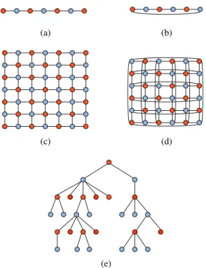
The path, ring (with an even number of vertices), and finite grid graphs, which are shown in Figure 1, are all examples of bipartite graphs and all have simple largest graph Lapla-cian eigenvalues. Using the largest eigenvector downsampling method leads to the elimination of every other vertex on the path and ring graphs, and to the quincunx sampling pattern on the finite grid graph (with or without boundary connections). Trees (acyclic, connected graphs) are also bipartite. An example of a tree is shown in Figure 1(e). Fix an arbitrary vertexr to be the root of the treeT, letY0
r be the singleton
set containing the root, and then define the sets {Yt
r}t=1,2,...
by Yt
r := {i∈ V :i isthops from the root vertex r inT }.
(a) (b)
(c) (d)
(e)
Fig. 1. Examples of partitioning structured graphs into two sets (red and blue) according to the polarity of the largest eigenvector of the graph Laplacian. For the path graph in (a) and the ring graph in (b), the method selects every other vertex like classical downsampling of discrete-time signals. For the finite grid graphs with the ends unconnected (c) and connected (d), the method results in the quincunx sampling pattern. For a tree graph in (e), the method groups the vertices at every other depth of the tree.
of the graph Laplacian splits the vertices of the tree into two sets according to the parity of the depths of the tree. That is, if we letYeven
r :=∪t=0,2,...YrtandYrodd:=∪t=1,3,...Yrt, then Yeven
r =V+ andYrodd=V−, or vice versa.
In related work, [18] and [19] suggest to downsample bipartite graphs by keeping all of the vertices in one subset of the bipartition, and [20] suggests to downsample trees by keeping vertices at every other depth of the tree. Therefore, the largest eigenvector downsampling method can be seen as a generalization of those approaches.
C. Connections with Graph Coloring and Spectral Clustering
A graph G = {V,E,W} is k-colorable if there exists a partition ofV into subsetsV1,V2, . . . ,Vk such that if vertices
i, j ∈ V are connected by an edge in E, then i andj are in different subsets in the partition. The chromatic number χ of a graph G is the smallest ksuch that G isk-colorable. Thus, the chromatic number of a graph is equal to 2 if and only if the graph is bipartite.
As we have seen with the examples in the previous section, when a graph is bipartite, it is easy to decide how to split it into two sets for downsampling. When the chromatic number of a graph is greater than two, however, we are interested in finding an approximate coloring [21]; that is, a partition that has as few edges as possible that connect vertices in the same
subset.2 As noted by [21], the approximate coloring problem is in some sense dual to the problem of spectral clustering (see, e.g. [22] and references therein).
Aspvall and Gilbert [21] suggest to construct an approx-imate 2-coloring of an unweighted graph according to the polarity of the eigenvector associated with the most negative eigenvalue of the adjacency matrix. For regular graphs, the eigenvector associated with the most negative eigenvalue of the adjacency matrix is the same as the largest graph Laplacian eigenvector, and so the method of [21] is equivalent to the largest Laplacian eigenvector method for that special case.
D. Connections with Nodal Domain Theory
A positive (negative) strong nodal domain of f on G is a maximally connected subgraph such thatf(i)>0 (f(i)<0) for all vertices i in the subgraph [17, Chapter 3]. A positive (negative) weak nodal domain of f on G is a maximally connected subgraph such that f(i) ≥ 0 (f(i) ≤ 0) for all vertices i in the subgraph, with f(i) 6= 0 for at least one vertexiin the subgraph.
A graph downsampling can be viewed as an assignment of positive and negative signs to vertices, with positive signs assigned to the vertices that we keep, and negative signs to the vertices that we eliminate. The goal of having few edges within either the removed set or the kept set is closely related to the problem of maximizing the number of nodal domains of the downsampling. This is because maximizing the number of nodal domains leads to nodal domains with fewer vertices, which results in fewer edges connecting vertices within the removed and kept sets.
Next, we briefly mention some general bounds on the number of nodal domains of eigenvectors of graph Laplacians: (ND1) u`has at most`weak nodal domains and`+s−1strong
nodal domains, wheresis the multiplicity ofλ`[23], [17, Theorem 3.1].
(ND2) The largest eigenvector umax has N strong and weak nodal domains if and only ifGis bipartite. Moreover, ifH
is an induced bipartite subgraph ofG with the maximum number of vertices, then the number of vertices inH is an upper bound on the number of strong nodal domains of any eigenvector of a generalized Laplacian ofG [17, Theorem 3.27].
(ND3) If λ` is simple and u`(i) 6= 0, ∀i ∈ V, the number of nodal domains of u` is greater than or equal to `−r,
wherer is the number of edges that need to be removed from the graph in order to turn it into a tree3[24].
Note that while both the lower and upper bounds on the number of nodal domains of the eigenvectors of graph Laplacians are monotonic in the index of the eigenvalue, the actual number of nodal domains is not always monotonic in the index of the eigenvalue (see, e.g., [25, Figure 1] for an example where they are not monotonic). Therefore, for arbitrary graphs, 2In other contexts, the termapproximate coloringis also used in reference to finding a properk-coloring of a graph in polynomial time, such thatkis as close as possible to the chromatic number of the graph.
3Berkolaiko proves this theorem for Schr¨odinger operators, which encom-pass generalized Laplacians of unweighted graphs.
it is not guaranteed that the largest eigenvector of the graph Laplacian has more nodal domains than the other eigenvectors. For specific graphs such as bipartite graphs, however, this is guaranteed to be the case, as can be seen from the above bounds and Theorem 1. Finally, in the case of repeated graph Laplacian eigenvalues, [17, Chapter 5] presents a hillclimbing algorithm to search for an associated eigenvector with a large number of nodal domains.
E. Alternative Graph Downsampling Methods
We briefly mention some alternative graph downsam-pling/partitioning methods:
1) As mentioned above, [21] partitions the graph based on the polarity of the eigenvector associated with the most negative eigenvalue of the adjacency matrix.
2) We can do a k-means clustering on umax with k = 2 to separate the sets. A closely related alternative is to set a non-zero threshold in (1). A flexible choice of the threshold can ensure that |V1| ≈N2.
3) In [8], Narang and Ortega downsample based on the solution to the weighted max-cut problem:
arg max V1 n cut(V1,V1c) o = arg max V1 ( X i∈V1 X i0∈Vc 1 Wii0 ) .
This problem is NP-hard, so approximations must be used for large graphs.
4) Barnard and Simon [26] choose V1 to be a maximal independent set (no edge connects two vertices in V1 and every vertex in Vc
1 is connected to some vertex in
V1). Maximal independent sets are not unique, but can be found via efficient greedy algorithms.
5) Ron et al. propose the SelectCoarseNodes algorithm [13, Algorithm 2], which leverages an algebraic distance measure to greedily select those nodes which have large future volume, roughly corresponding to those nodes strongly connected to vertices in the eliminated set. Additionally, there are a number of graph coarsening methods where the reduced set of vertices is not necessarily a subset of the original set of vertices. We discuss those further in Section IV-E.
IV. GRAPHREDUCTION
So we now have a way to downsample a graph to a subset of the vertices. However, in order to implement any type of multiscale transform that will require filtering operations defined on the subset of selected vertices, we still need to define a method to reduce the graph Laplacian on the original set of vertices to a new graph Laplacian on the subset of selected vertices. We refer to this process asgraph reduction. For the purpose of mutliscale transforms, we would ideally like the graph reduction method to have some or all of the properties listed below. Note that the following represents one example of desiderata and is neither exhaustive nor definitive. (GR1) The reduction is in fact a graph Laplacian (i.e., a symmet-ric matrix with row sums equal to zero and nonpositive off-diagonal elements).
(GR2) It preserves connectivity. That is, if the original graph is connected, then the reduced graph is also connected. (GR3) The spectrum of the reduced graph Laplacian is
repre-sentative of and contained in the spectrum of the original graph Laplacian.
(GR4) It preserves structural properties (e.g., if the original graph is a tree or bipartite, the reduced graph is accord-ingly a tree or bipartite).
(GR5) Edges in the original graph that connect vertices in the reduced vertex set are preserved in the reduced graph. (GR6) It is invertible or partially invertible with some side
information; i.e., from the reduced graph Laplacian and possibly some other stored information, we can recover the original graph Laplacian.
(GR7) It is computationally efficient to implement.
(GR8) It preserves graph sparsity. That is, the ratio of the number of edges over potential edgesN(N|E|−1)/2does not increase too much from the original graph to the reduced graph. In addition to preserving computational benefits associated with sparse matrix-vector multiplica-tion, keeping this ratio low ensures that the reduced graph also captures local connectivity information and not just global information.
(GR9) There is some meaningful correspondence between the eigenvectors of the reduced graph Laplacian and the orig-inal graph Laplacian; for example, when restricted to the kept set of vertices, the lowest (smoothest) eigenvectors of the original Laplacian are similar to or the same as the eigenvectors of the reduced Laplacian.
In the following, we discuss in detail one particular choice of graph reduction that satisfies some, but not all, of these properties. In Section IV-E, we briefly mention a few other graph reduction methods.
A. Kron Reduction
The starting point for the graph reduction method we con-sider here is Kron reduction (see [27] and references therein). We start with a weighted graphG={V,E,W}, its associated graph LaplacianL, and a subsetV1 (V of vertices (the set
selected by downsampling, for example) on which we want to form a reduced graph.4 The Kron reduction of Lis the Schur complement [28] of L relative to LVc
1,V1c; that is, the Kron
reduction ofL is given by K(L,V1) :=LV1,V1− LV1,V1cL −1 Vc 1,V1cLV c 1,V1, (3)
where LA,B denotes the |A| × |B| submatrix consisting
of all entries of L whose row index is in A and whose column index is in B. We can also uniquely associate with LKron−reduced = K(L,V
1) a reduced weighted graph
GKron−reduced =
V1,EKron−reduced,WKron−reduced by letting WijKron−reduced= ( −LKron−reduced ij ifi6=j, 0 o.w. , (4) 4We assume|V 1| ≥2.
and takingEKron−reducedto be the set of edges with non-zero
weights in (4).5 An example of Kron reduction is shown in
Figure 2. 2 2 11 1 11 9 11 9 2 9 16 27 2 3 9 4 3 2 15 8 4 2 10 2 4 4 1 9 6 6 6 6 6 6 6 6 2 2 6 1 Kron
Fig. 2. An example of Kron reduction. The vertices inV1 are in red, and
those inVc
1 are in blue.
B. Properties of Kron Reduction
For a complete survey of the topological, algebraic, and spectral properties of the Kron reduction process, see [27]. In the next theorem, we summarize the results of [27] that are of most interest with regards to multiscale transforms.
Theorem2 (D¨orfler and Bullo, 2013): Let L be a graph Laplacian of an undirected weighted graph G on the vertex set V, V1 ( V be a subset of vertices with |V1| ≥ 2,
LKron−reduced=K(L,V
1)be the Kron-reduced graph Lapla-cian defined in (3), andGKron−reducedbe the associated
Kron-reduced graph. Then
(K1) The Kron-reduced graph Laplacian in (3) is well-defined (K2) LKron−reduced is indeed a graph Laplacian
(K3) If the original graphG is connected (i.e.,λ1(L)>0), then the Kron-reduced graph GKron−reduced is also
connected(i.e., λ1(LKron−reduced)>0)
(K4) If the original graphGis loopless, then the Kron-reduced graphGKron−reduced is also loopless6
(K5) Two verticesi, j∈ V1 are connected by an edge if and only if there is a path between them inGwhose vertices all belong to{i, j} ∪ Vc
1
(K6) Spectral interlacing: for all`∈ {0,1, . . . ,|V1| −1},
λ`(L)≤λ`(LKron−reduced)≤λ
`+|V|−|V1|(L). (5)
In particular, (5) and property (K4) above imply
0 =λmin(L) =λmin(LKron−reduced)
≤λmax(LKron−reduced)≤λmax(L) (6) (K7) Monotonic increase of weights: for all i, j ∈ V1,
WijKron−reduced≥Wij
(K8) Resistance distance [29] preservation: for alli, j∈ V1,
dRG(i, j) := (δi−δj)TL†(δi−δj)
= (δi−δj)T(LKron−reduced)†(δi−δj),
where L† is the pseudoinverse of L and δi is the
Kronecker delta (equal to 1 at vertexiand 0 at all other vertices)
5In (4), we still index the new weights by the same vertex indicesiandj. In practice, the vertices iandjwill receive new ordinal indices between 1
andNKron−reduced=|V
1|, the number of vertices in the reduced graph.
6While [27] considers the more general case ofloopy Laplacians, the graphs we are interested in are allloopless; that is, there are no self-loops connecting a vertex to itself, and thereforeLnn=P
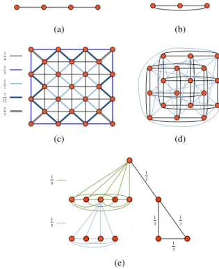
i∈V,i6=nWni. (a) (b) 3 2 3 1 2 1 4 1 12 7 (c) (d) 6 1 2 1 3 1 3 1 3 1 5 1 (e)
Fig. 3. Kron reductions of the graphs of Figure 1, with the blue vertices eliminated. If the weights of all of the edges in the original path and ring graphs are equal to 1, then the weights of all of the edges in the Kron-reduced graphs in (a) and (b) are equal to12. For the Kron reduction of the finite grid graph with the ends connected (d), the weights of the blue edges are equal to
1
2 and the weights of the black edges are equal to 1
4. The weights of Kron
reductions of the finite grid graph with the ends unconnected (c) and the tree graph (e) are shown by color next to their respective Kron reductions.
C. Special Cases
As in Section III-B for the vertex selection process, we analyze the effect of Kron reduction on some special classes of graphs in order to (i) provide further intuition behind the graph reduction process; (ii) show that Kron reduction is a generalization of previously suggested techniques for reducing graphs belonging to these special classes; and (iii) highlight both the strengths and weaknesses of this choice of graph reduction.
1) Paths: The class of path graphs is closed under the sequential operations of largest eigenvector vertex selection and Kron reduction. That is, if we start with a path graphGP
withN vertices, and select a subsetV1according the polarity of the largest eigenvector of the graph Laplacian ofGP, then
the graph associated withK(GP,V1)is also a path graph. If the weights of the edges of the original graph are all equal to
1, the weights of the edges of the Kron-reduced graph are all equal to 12. The Kron reduction of the graph shown in Figure 1(a) is shown in Figure 3(a).
2) Rings: The Kron reduction of the ring graph shown in Figure 1(b) is shown in Figure 3(b). It is a ring graph with half the number of vertices, and the weights of the edges are also halved in the Kron reduction process.
3) Finite Grids: The Kron reductions of the finite grid graphs shown in Figure 1(c,d) are shown in Figure 3(c,d). If we rotate Figure 3(c) clockwise by ninety degrees, we see that it is a subgraph of the 8-connected grid. We do not consider
graphs with infinite vertices here, but the combined effect of the largest eigenvector vertex selection and Kron reduction operations is to map an infinite (or very large) 4-connected grid to an 8-connected grid.
4) Trees: The Kron reduction of the tree shown in Figure 1(e) is shown in Figure 3(e). Note that the Kron reduction of a tree is not a tree because siblings in the original graph are connected in the Kron-reduced graph. However, it does have a particular structure, which is a union of complete subgraphs. For every node i in the reduced graph, and each one of that node’s children j in the original graph, there is a complete subgraph in the reduced graph that includes i and all of the children of j (i.e., the grandchildren of i through j). If the weights of the edges in the original graph are equal to one, then the weights in each of the complete subgraphs are equal to one over the number of vertices in the complete subgraph. This class of graphs highlights two of the main weaknesses of the Kron reduction: (i) it does not always preserve regular structural properties of the graph; and (ii) it does not always preserve the sparsity of the graph. We discuss a sparsity-enhancing modification in Section IV-D.
5) k-Regular Bipartite Graphs: In [18], Narang and Ortega consider connected and unweightedk-RBGs.7They
downsam-ple by keeping one subset of the bipartition, and they construct a new graph on the downsampled vertices V1 by linking vertices in the reduced graph with an edge whose weight is equal to the number of their common neighbors in the original graph. If the vertices of the original graph are rearranged so that all the vertices in V1 have smaller indices than all the vertices in Vc
1, the adjacency and Laplacian matrices of the original graph can be represented as:
W= 0 W1 WT 1 0 andL= " kIN 2 −W1 −WT 1 kIN 2 # . (7) Then for all i, j ∈ V1 (with i 6=j), the (i, j)th entry of the adjacency matrix of the reduced graph is given by
WijkRBG−reduced(V1) = (W1WT1)ij. (8)
They also show that
LkRBG−reduced(V1) =k2IN
2 −W1W
T
1. (9)
Now we examine the Kron reduction ofk-RBGs. The Kron-reduced Laplacian is given by:
LKron−reduced(V 1) =LV1,V1− LV1,V1cL −1 Vc 1,V1cLV c 1,V1 =kIN 2 −(−W1)(kI N 2) −1(−WT 1) =kIN 2 − 1 kW1W T 1,
which is a constant factor 1k times the reduced Laplacian (9) of [18]. So, up to a constant factor, the Kron reduction is a generalization of the graph reduction method presented in [18] for the special case of regular bipartite graphs.
7Although [18] considers unweightedk-RBGs, the following statements also apply to weighted k-RBGs if we extend the definition of the reduced adjacency matrix (8) to weighted graphs.
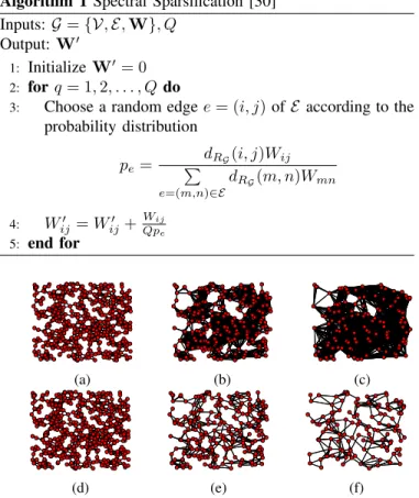
Algorithm 1 Spectral Sparsification [30] Inputs:G={V,E,W}, Q
Output:W0
1: Initialize W0= 0
2: forq= 1,2, . . . , Qdo
3: Choose a random edgee= (i, j)ofE according to the probability distribution pe= dRG(i, j)Wij P e=(m,n)∈E dRG(m, n)Wmn 4: Wij0 =Wij0 +Wij Qpe 5: end for (a) (b) (c) (d) (e) (f)
Fig. 4. Incorporation of a spectral sparsification step into the graph reduction. (a)-(c) Repeated largest eigenvector downsampling and Kron reduction of a sensor network graph. (d)-(f) The same process with the spectral sparsification of [30] used immediately after each Kron reduction.
D. Graph Sparsification
As a consequence of property (K5), repeated Kron reduction often leads to denser and denser graphs. We have already seen this loss of sparsity in Section IV-C4, and this phenomenon is even more evident in larger, less regular graphs. In addition to computational drawbacks, the loss of sparsity can be im-portant, because if the reduced graphs become too dense, they may not effectively capture the local connectivity information that is important for processing signals on the graph. There-fore, in many situations, it is advantageous to perform graph sparsification immediately after the Kron reduction as part of the overall graph reduction phase.
There are numerous ways to perform graph sparsification. In this paper, we use a straightforward spectral sparsification algorithm of Spielman and Strivastava [30], which is described in Algorithm 1. This sparsification method pairs nicely with the Kron reduction, because [30] shows that for large graphs and an appropriate choice of the number of samples Q, the graph Laplacian spectrum and resistance distances between vertices are approximately preserved with high probability. In Figure 4, we show an example of repeated downsampling followed by Kron reduction and spectral sparsification.
E. Alternative Graph Reduction Methods
1) In [8], Narang and Ortega define a reduced graph via the weighted adjacency matrix by taking W(j+1) =
[W(j)]2
V1,V1. Here,[W
(j)]2 represents the 2-hop ad-jacency matrix of the original graph. The reduced Lapla-cian can then be defined asL(j+1)=D(j+1)−W(j+1), where D(j+1) is computed from W(j+1). However, there are a number of undesirable properties of this reduction method. First, and perhaps foremost, the re-duction method does not always preserve connectivity. Second, self-loops are introduced at every vertex in the reduced graph. Third, vertices in the selected subset that are connected by an edge in the original graph may not share an edge in the reduced graph. Fourth, the spectrum of the reduced graph Laplacian is not necessarily contained in the spectrum of the original graph Laplacian.
2) Ron et al. [13] assign a fraction Pij of each vertex i in the original graph to each vertex j ∈ V1 in the reduced graph that is close toiin the original graph (in terms of an algebraic distance). The assignment satisfies
P
j∈V1Pij = 1for alli∈ V andPjj = 1for allj∈ V1,
and for each eliminated vertex i ∈ Vc
1, an upper limit is placed on the number of vertices j ∈ V1 that have
Pij >0. Then for allj, j0∈ V1,
Wjjreduced0 := X
m,n∈V,m6=n
PmjPnj0Wmn.
Next, we mention some graph coarsening (also called coarse-graining) methods that combine graph downsampling and reduction into a single operation by forming aggregate nodes at each resolution, rather than keeping a strict subset of original vertices. The basic approach of these methods is to partition the original set of vertices into clusters, represent each cluster of vertices in the original graph with a single vertex in the reduced graph, and then use the original graph to form edges and weights that connect the representative vertices in the reduced graph. Some examples include:
1) Lafon and Lee [31] cluster based on diffusion distances and form new edge weights based on random walk transition probabilities.
2) The Lean Algebraic Multigrid (LAMG) method of [32] builds each coarser Laplacian by selecting seed nodes, assigning each non-seed node to be aggregated with exactly one seed node, and setting the weights between two new seed nodesj andj0 to be
Wjjreduced0 := X i∈Vj X i0∈V j0 Wii0,
where Vj and Vj0 are the sets of vertices that have
been aggregated with seeds j and j0, respectively. The seed assignments are based on an affinity measure that approximates short time diffusion distances, rather than the algebraic distances used in [13].
3) Multilevel clustering algorithms such as those presented in [33], [34] often use greedy coarsening algorithms such as heavy edge matching or max-cut coarsening (see [33, Section 3] and [34, Section 5.1] for details).
For more thorough reviews of the graph partitioning and coarsening literature, see, e.g., [11], [13], [35].
To summarize, given a graph G and a desired number of resolution levels, in order to generate a multiresolution of graphs, we only need to choose a downsampling operator and a graph reduction method. In the remainder of the paper, we use the largest eigenvector downsampling operator and the Kron reduction with the extra sparsification step to generate graph multiresolutions such as the three level one shown in Figure 4(d)-(f). Note that graph multiresolutions generated in this fashion are completely independent of any signals residing on the graph.
V. FILTERING ANDINTERPOLATION OFGRAPHSIGNALS Equipped with a graph multiresolution, we now proceed to analyze signals residing on the finest graph in the multiresolu-tion. The two key graph signal processing components we use in the proposed transform are a generalized filtering operator and an interpolation operator for signals on graphs. Filters are commonly used in classical signal processing analysis to separate a signal into different frequency bands. In this section, we review how to extend the notion of filtering to graph signals. We focus on graph spectral filtering, which leverages the eigenvalues and eigenvectors of Laplacian operators from spectral graph theory [36] to capture the geometric structure of the underlying graph data domain. We then discuss different methods to interpolate from a signal residing on a coarser graph to a signal residing on a finer graph whose vertices are a superset of those in the coarser graph.
A. Graph Spectral Filtering
A graph signalis a function f :V →R that associates a
real value to each vertex of the graph. Equivalently, we can view a graph signal as a vectorf ∈RN.
In frequency filtering, we represent signals as linear com-binations of a set of signals and amplify or attenuate the contributions of different components. In classical signal pro-cessing, the set of component signals are usually the complex exponentials, which carry a notion of frequency and give rise to the Fourier transform. In graph signal processing, it is most common to choose the graph Fourier expansion basis to be the eigenvectors of the combinatorial or normalized graph Laplacian operators. This is because the spectra of these graph Laplacians also carry a notion of frequency (see, e.g., [2, Figure 3]), and their eigenvectors are the graph analogs to the complex exponentials, which are the eigenfunctions of the classical Laplacian operator.
More precisely, the graph Fourier transform with the com-binatorial graph Laplacian eigenvectors as a basis is
ˆ f(λ`) :=hf,u`i= N X i=1 f(i)u∗`(i), (10) and agraph spectral filter, which we also refer to as a kernel, is a real-valued mappingˆh(·)on the spectrum of graph Laplacian eigenvalues. Just as in classical signal processing, the effect of the filter is multiplication in the Fourier domain:
ˆ
or, equivalently, taking an inverse graph Fourier transform, fout(i) = N−1 X `=0 ˆ fin(λ`)ˆh(λ`)u`(i). (12) We can also write the filter in matrix form as fout =Hfin,
whereH is a matrix function [37]
H= ˆh(L) =U[ˆh(Λ)]U∗, (13) where ˆh(Λ) is a diagonal matrix with the elements of the diagonal equal to {ˆh(λ`)}`=0,1,...,N−1. We can also use the normalized graph Laplacian eigenvectors as the graph Fourier basis, and simply replace L,λ`, andu` by L˜, ˜λ`, and u˜` in
(10)-(13). A discussion of the benefits and drawbacks of each of these choices for the graph Fourier basis is included in [2].
B. Alternative Filtering Methods for Graph Signals
We briefly mention two alternative graph filtering methods: 1) We can filter a graph signal directly in the vertex domain by writing the output at a given vertex i as a linear combination of the input signal components in a neighborhood of i. Graph spectral filtering with an order K polynomial kernel can be viewed as filtering in the vertex domain with the component of the output at vertex iwritten as a linear combination of the input signal components in a K-hop neighborhood of i (see [2] for more details).
2) Other choices of filtering bases can be used in place of
L in (13). For example, in [38], [39], Sandryhaila and Moura examine filters that are polynomial functions of the adjacency matrix.
C. Interpolation on Graphs
Given the values of a graph signal on a subset, V1, of the vertices, the interpolation problem is to infer the values of the signal on the remaining vertices, V1c = V\V1. It is usually assumed that the signal to be interpolated is smooth. This assumption is always valid in our construction, because the signals we wish to interpolate have been smoothed via a lowpass graph spectral filter.
We use the interpolation model of Pesenson [40], which is to interpolate the missing values, fVc
1, of the signal f by
writing the interpolant as a linear combination of the Green’s functions of the regularized graph Laplacian,L¯:=L+I, that are centered at the vertices in V1.8 That is, the interpolation is given by
finterp =
X
j∈Vr
α[j]ϕj=ΦV1α, (14)
whereϕj is a Green’s kernelˆg(λ`) =λ1
`+translated to center
vertex j (see [5], [2] for more on generalized translation on graphs): ϕj =Tjg= ˆg(L)δj=U[ˆg(Λ)]U∗δj = |V|−1 X `=0 1 λ`+u ∗ `(j)u`,
8Pesenson’s model and subsequent analysis in [40] is for any powerL¯tof
the regularized Laplacian, but we stick tot= 1throughout for simplicity.
andΦV1 is a |V| × |V1| matrix with columns {ϕj}j∈V1. We
display three such translated Green’s functions in Figure 5. Note that these are localized functions satisfying the property
¯
Lϕj=U[Λ+I]U∗U[ˆg(Λ)]U∗δj= ¯LL¯−1δj =δj. The parameter controls the spread of the translated Green’s functions around their center vertices, with a smaller value of
leading to larger spreads.
0 0.2 0.4 0.6 0.8 1 1.2 1.4 1.6 1.8 2 0 0.5 1 1.5 0 0.5 1 1.5 2 2.5 3 3.5
Fig. 5. Three localized Green’s functions, centered at different vertices on the Minnesota graph.
To perform the interpolation, we find the coefficientsαsuch that the linear combination of Green’s functions restricted to the subsetV1of vertices yields the signal values on this subset: fV1 =ΦV1,V1α∗, (15)
where fV1 is a vector containing the values of the signal on
the vertices in V1, andΦV1,V1 is the submatrix that contains
only the rows ofΦV1 corresponding to the vertices inV1. To
compute α∗=Φ−V11,V1fV1, we note that
ΦV1,V1= L¯ −1 V1,V1 =hL¯V1,V1−L¯V1,V1c ¯ LVc 1,V1c −1 ¯ LVc 1,V1 i−1 ,
where the last equality follows from the Matrix Inversion Lemma. Thus, the cost to compute
α∗= h ¯ LV1,V1−L¯V1,V1c ¯ LVc 1,V1c −1 ¯ LVc 1,V1 i fV1 (16)
is dominated by the solution of a sparse diagonally dominant set of |V| − |V1| linear equations. Finally, we can substitute
α∗back into (14) to find the interpolated signal, whose values
on V1 of course correspond to the given values fV1. This
last calculation can be approximated efficiently by upsampling
α∗ to V, and filtering it with the Green’s kernel g(·)ˆ using
the polynomial approximation algorithm discussed in Section VII-C. Pesenson [40] refers to the interpolated signalfinterp as
avariational spline.
As a brief aside, we note that the matrix in (16) is exactly the Kron reduction K( ¯L,V1)of the regularized graph Laplacian on the set of vertices V1 where the signal values are known.
As with downsampling and graph reduction, there are a number of different methods to interpolate smooth signals on graphs, and we briefly mention a few alternatives here:
1) Graph-based semi-supervised learning methods, such as Tikhonov regularization (see, e.g., [41]-[46]). Like many of those methods, the spline interpolation method we use can be viewed as solving an optimization problem (see [40]). One main difference is that in our multiscale transform, we will usually have approximately half of the signal values available, whereas the number of
9
signal values available in the semi-supervised learning literature is usually assumed to be significantly smaller. 2) Grady and Schwartz’s anisotropic interpolation solves
the system of equations LVc
1,V1cfV1c = −LV1c,V1fV1 in
order to minimizefT
interpLfinterpsubject tofinterp(i) =f(i)
for alli∈ V.
3) Rather than using the Green’s functions as the inter-polating functions in (14), Narang et al. [47], [48] use the eigenvectors of the normalized graph Laplacian associated with the lowest eigenvalues.
VI. A PYRAMIDTRANSFORM FORSIGNALS ONGRAPHS We are finally ready to combine the downsampling, graph reduction, filtering, and interpolation operations from the pre-vious three sections to define a multiscale pyramid transform for signals on graphs. After reviewing the classical Laplacian pyramid, we summarize our extension, first for a single level and then for the whole pyramid.
A. The Classical Laplacian Pyramid
In [15], Burt and Adelson introduce the Laplacian pyramid. Originally designed with image coding in mind, the Laplacian pyramid is a multiresolution transform that is applicable to any regularly-sampled signal in time or space. A schematic representation of a single level of the Laplacian pyramid is shown in Figure 6(a). At each level of the pyramid, an input signalxis lowpass filtered (H) and then downsampled to form a coarse approximation of the original signal. A prediction of the input signal is then formed by upsampling and lowpass filtering (G) the coarse approximation. The prediction errory, i.e., the difference between the input signal and the prediction based on the coarse approximation, is stored for reconstruc-tion. This process is iterated, with the coarse approximation that is output at the previous level acting as the input to the next level. The sequencex(i)
i=1,2,... represents a series of
coarse approximations of the original signalx(0)at decreasing resolutions. If, for example, the downsampling is by a factor of 2 and the original signal x(0)∈
RN, thenx(i)∈R2 −iN
. The lowest resolution approximation, x(J), of the original signal and the sequence of prediction errors,
y(i) i=0,1,...,J−1 are stored and/or transmitted for recon-struction. Therefore, the Laplacian pyramid is an overcomplete transform, as a J-level pyramid downsampled by a factor of κ at each level maps an input of dimension N into
N1− 1 κ J+1 1−1 κ
transform coefficients. On the other hand, the Laplacian pyramid has a number of desirable properties. First, perfect reconstruction of the original signal is possible for any choice of filtering operations H and G. It is easy to see that upsampling x(j+1), filtering it by G, and summing with the prediction error y(j) yields the finer approximation x(j). Second, the prediction errors usually have less entropy than the original signal of the same dimension, enabling further compression. Third, it is computationally efficient to implement the transform, due to the hierarchical and local nature of the computations.
For some applications, the reconstruction process starts with noisy transform coefficients, due to communication noise,
̶ x(j) H ↓ ↑ G + x(j+1) y(j) (a) Interpolate from Ѵ1 toѴ ̶ x(j)
L (j) Selec4on Vertex m Reduc4on Graph (j) L (j+1) H(j) x(j+1) y(j) m(j) ↓Ѵ1 + (b) x(4) Single Level of Pyramid x(0) L (0) L (1) x(1) y(0) m(0) Single Level of Pyramid L (2) x(2) y(1) m(1) Single Level of Pyramid L (3) x(3) y(2) m(2) Single Level of Pyramid m(3) Ly (4) (3) (c)
Fig. 6. (a) A single level of the classical Laplacian pyramid of Burt and Adelson [15]. (b) A single level of the pyramid scheme proposed for signals defined on graphs. The top half consisting of the graph downsampling and reduction is specific to the graph (but the same for every signal on that graph), while the bottom half is specific to each graph signal. (c) A multilevel pyramid for signals defined on graphs.
quantization error, or other types of processing. In this case, Do and Vetterli [49], [50] show that Burt and Adelson’s single-level synthesis operator is not optimal in terms of the reconstruction error. The single-level analysis operator that transforms a coarse approximation x(j) into the next coarse approximation x(j+1) and prediction error y(j) is a
frame operator (see, e.g., [51]). Frame operators have an infinite number of left inverses, but the one that minimizes the reconstruction error is the pseudoinverse of the analysis operator at each level of the pyramid. In Section VI-D, we also use the pseudoinverse of the analysis operator as the synthesis operator at each level of our Laplacian pyramid for signals on graphs. Thus, we defer a more precise mathematical treatment of the optimal reconstruction until then.
B. The Analysis Operator for a Single Level of the Pyramid for Signals on Graphs
We now extend the classical Laplacian pyramid to a pyramid transform for signals on graphs. At each level of the pyramid, the inputs are the current coarse approximation,x(j)∈RN
(j)
, of the original signal, and the current graph LaplacianL(j)∈ RN
(j)
×RN (j)
ofL(j), as described in Section III, to select the vertices of the graph on which to form the reduced graph at resolution scale
j+ 1. We denote the output of the vertex selection process by m(j)∈ RN (j) , where m(j)(i) =
1, if vertex iis selected to be included in the reduced graph
0, otherwise
.
The vertex selection vectorm(j) is used both to reduce the graph and to define the downsampling and interpolation oper-ators. For graph reduction, we use Kron reduction followed by spectral sparsification, as discussed in Section IV. The graph Laplacian of the reduced graph is given by
L(j+1)=SKL(j),m(j) =S L(j) V(j) 1 ,V (j) 1 − L(j) V(j) 1 ,V (j)c 1 L(j) V(j)c 1 ,V (j)c 1 −1 L(j) V(j)c 1 ,V (j) 1 ! , whereV1(j):= i∈ {1,2, . . . , N(j)}:m(j)(i) = 1 andS is the spectral sparsification operator. The reduced graphL(j+1) and the vertex selection vector m(j), both of which need to be stored for reconstruction, are the first two outputs of the transform at each level of the pyramid.
The other two outputs are the coarse approximation vector x(j+1)at the coarser resolution scalej+1, and the next predic-tion error vectory(j). The course approximation vector is com-puted in a similar fashion as in the classical Laplacian pyramid, with the filtering and downsampling operators replaced by their graph analogs. The downsampling operator↓corresponds to matrix multiplication by the matrixS(dj)∈RN(j+1)×
RN (j)
, where S(dj) := [IN(j)]
V1(j),V(j) and IN(j) is an N(j)×N(j)
identity matrix. For example, ifm(j)= (1,1,0,0,1,0)T, then
S(dj)= 1 0 0 0 0 0 0 1 0 0 0 0 0 0 0 0 1 0 .
Rather than upsample and filter with another lowpass filterG
as in the classical pyramid, we compute the prediction error with the spline interpolation method of Section V-C. While this adds some additional computational cost, our experiments showed that this change significantly improves the predictions, and in turn the sparsity of the transform coefficients. So the single-level analysis operatorT(aj):RN
(j) →RN(j)+N(j+1) is given by T(aj)x(j):= S(dj)H(j) IN(j)−Φ (j) V1 Φ(Vj) 1,V1 −1 S(dj)H(j) x (j) = x(j+1) y(j) (17) In (17), the filtering operator isH(j)=U(j)[ˆh(Λ(j))]U(j)∗.
A schematic representation of a single level of the pyramid for signals on graphs is shown in Figure 6(b). Note that while we use the polarity of the largest eigenvector of the graph Laplacian as a vertex selection method, the sparsified Kron reduction as a graph reduction method, the eigenvectors
of the graph Laplacian as a filtering basis, and the spline interpolation method with translated Green’s functions, other vertex selection, graph reduction, filtering, and interpolation methods can be substituted into these blocks without affecting the perfect reconstruction property of the scheme.
C. The Multilevel Pyramid
The multilevel pyramid for signals on graphs is shown in Figure 6(c). As in the classical case, we iterate the single-level analysis on the downsampled output of the lowpass channel. In (17), the filtering operatorsH(j) necessarily depend on the resolution scalejthrough their dependence on the eigenvectors and eigenvalues ofL(j). However, the filterˆh: [0, λ(0)
max]→R
may be fixed across all levels of the pyramid due to property (6) of the Kron reduction, which guarantees that the spectrum of L(j) is contained in[0, λ(0)
max]for allj.9
D. Synthesis Operators for a Single Level and Optimal Re-construction
Just as is the case in the classical Laplacian pyramid, for any choices of filter ˆh(·), we can reconstruct x(j) perfectly from x(j+1) and y(j) with a single-level synthesis operator, T(sj):RN (j)+N(j+1) →RN (j) , given by T(sj) x(j+1) y(j) := Φ(Vj) 1 Φ(Vj) 1,V1 −1 IN(j) x(j+1) y(j) . (18) Note that in order to apply the synthesis operator T(sj), we
need access to both L(j) and m(j), which are used for the interpolation.
It is straightforward to check that T(sj)T
(j)
a = IN(j),
guaranteeing perfect reconstruction. However, once again anal-ogously to the classical Laplacian pyramid, when noise is introduced into the stored coefficients x(j+1) and y(j), we would like to reconstruct with the pseudoinverse ofT(aj):
T(aj)† :=
T(aj)∗T(aj)
−1
T(aj)∗. (19)
If x˜(j+1) and y˜(j) are the noisy versions of x(j+1) and y(j), respectively, then ˘x(j) =T(j)† a hx˜(j+1) ˜ y(j) i minimizes the reconstruction error. That is,
T(aj)† x˜(j+1) ˜ y(j) = argmin x∈RN(j) T(aj)x− ˜x(j+1) ˜ y(j) 2 . (20) For large graphs, rather than form and compute the matrix inverse in (19), it may be more computationally efficient to approximate the left-hand side of (20) with Landweber iteration [54, Theorem 6.1].
To summarize, for a multilevel pyramid for signals on graphs that hasJ resolution levels, the reconstruction process 9If we include spectral sparsification in the graph reduction step, then the spectrum ofL(j)is not guaranteed to be contained in[0, λ(0)
max]; however, for
large graphs, the results of [30] limit the extent to which the maximum graph Laplacian eigenvalue can increase beyondλ(0)max. In any case, we usually
define the filters on the entire positive real line, in which case there is no issue with the length of the spectrum increasing at successive levels of the pyramid.
−1 −0.8 −0.6 −0.4 −0.2 0 0.2 0.4 0.6 0.8 1 −1 −0.8 −0.6 −0.4 −0.2 0 0.2 0.4 0.6 0.8 1 −1 −0.8 −0.6 −0.4 −0.2 0 0.2 0.4 0.6 0.8 1 −1 −0.8 −0.6 −0.4 −0.2 0 0.2 0.4 0.6 0.8 1 Coarse Approximations Original Signal - x(0) Prediction Errors x(1) x(2) x(3) y(0) y(1) y(2) −1 −0.8 −0.6 −0.4 −0.2 0 0.2 0.4 0.6 0.8 1 −1 −0.8 −0.6 −0.4 −0.2 0 0.2 0.4 0.6 0.8 1 −1 −0.8 −0.6 −0.4 −0.2 0 0.2 0.4 0.6 0.8 1
Fig. 7. Three-level pyramid analysis of a piecewise-constant signal on the Minnesota road network of [52]. The number of vertices is reduced in successive coarse approximations fromN= 2642to1334to669to337. The overall redundancy factor of the transform in this case is 1.89.
−4 −3 −2 −1 0 1 2 3 4 −4 −3 −2 −1 0 1 2 3 4 −4 −3 −2 −1 0 1 2 3 4 −6 −5 −4 −3 −2 −1 0 1 2 Coarse Approximations Original Signal - x(0) Prediction Errors x(1) x(2) x(3) y(0) y(1) y(2) −6 −5 −4 −3 −2 −1 0 1 2 −6 −5 −4 −3 −2 −1 0 1 2 −6 −5 −4 −3 −2 −1 0 1 2
Fig. 8. Three-level pyramid analysis of a piecewise-smooth signal on the Stanford Bunny graph of [53]. The number of vertices is reduced in successive coarse approximations fromN= 8170to4108to2050to1018. The overall redundancy factor of the transform in this case is 1.88.
begins with knowledge ofm(0),m(1),. . .,m(J−1),L(0),L(1),
. . ., L(J−1), y(0), y(1), . . ., y(J−1), and x(J). We first use m(J−1) andL(J−1)to applyT(J−1)† a to h x(J) y(J−1) i . The result isx˘(J−1). We then usem(J−2)andL(J−2)to applyT(J−2)†
a
toh˘xy((JJ−−1)2) i
in order to compute˘x(J−2). We iterate this process
J times until we finally computex˘(0), which, if no noise has been introduced into the transform coefficients, is equal to the original signal x(0).
E. Illustrative Examples
In Figure 7, we use the proposed pyramid transform to analyze a piecewise-constant signal (the Fiedler vectoru1) on the Minnesota road network of [52]. After each Kron reduction at stage j, we use the spectral sparsification of Algorithm 1 withQset to the integer closest to4N(j)log(N(j)). The graph spectral filter is ˆh(λ`) := 0.5+0.5λ
`, and we take = 0.005
to form the regularized Laplacian for interpolation. We see
that the prediction error coefficients are extremely sparse, and those with non-zero magnitudes are concentrated around the discontinuity in the graph signal.
In Figure 8, we apply the transform to a piecewise smooth signal on the Stanford Bunny graph [53] with 8170 vertices. The signal is comprised of two different polynomials of the coordinates: x¯2+ ¯y−2¯z on the head and ears of the bunny, and ¯x−y¯+ 3¯z2−5 on the lower body, where (¯x,y,¯ z)¯ are the physical coordinates of each vertex. Since the graph is larger and the graph Laplacian spectrum is wider than the previous example, we take Q to be the integer closest to
16N(j)log(N(j)), the lowpass filter to be ˆh(λ`) := 5
5+λ`,
and= 0.05 for interpolation.
As a compression example, we hard threshold the 15346 pyramid transform coefficients of the signal, keeping only the 2724 with the largest magnitudes (approximately 1/3 the size of the original signal) and setting the rest to 0. Reconstruction of the signal from the thresholded coefficients yields an error
−6 −5 −4 −3 −2 −1 0 1 2 (a) 0 200040006000 800010000 12000 1400016000 0 1 2 3 4 5 6 (b) −6 −5 −4 −3 −2 −1 0 1 2 (c)
Fig. 9. Compression example. (a) The original piecewise-smooth signal with a discontinuity on the Stanford bunny [53]. (b) The sorted magnitudes of the 15346 pyramid transform coefficients. (c) The reconstruction from the 2724 coefficients with the largest magnitudes, using the least squares synthesis (19).
||freconstruction−f||2
||f||2 of 0.145 with the direct synthesis (18), and an
error of 0.086 with the least squares synthesis (19). Figure 9 shows the original signal, the sorted magnitudes of the transform coefficients, and the reconstruction with the least squares synthesis operator.
F. Comparison with Other Transforms
A thorough comparison of our proposed pyramid transform to other multiscale transforms for signals on graphs investi-gating which transforms work best on which types of graph signals in which signal processing tasks is beyond the scope of this work. However, in this section, we present a few illustrative numerical denoising and compression experiments with our proposed pyramid transform and other multiscale transforms for graph signals.
First, one qualitative difference between the proposed trans-form and many other multiscale transtrans-forms for graph signals is that our transform outputs both a multiresolution of graphs and a graph signal multiresolution residing on that graph multiresolution. While less important for numerical graph signal processing and machine learning tasks, this feature is especially beneficial for multiscale visualization of graph signals (e.g., the sequence of coarse approximations in the top row of Figure 8). A few other transforms such as the critically-sampled spline wavelet filter banks [9] share this feature, but many others such as the spectral graph wavelets [5] and the spatial graph wavelets [3] do not yield such a sequence of coarse approximations at different resolution levels.
Second, the dictionary atoms we construct tend to be jointly localized in the vertex domain and the graph spectral domain. The hope is that such atoms are able to sparsely represent various classes of graph signals, such as those that are piecewise smooth with discontinuities. Unfortunately, there is little theory to date relating mathematical classes of graph signals to the sparsity of particular transform coefficients. One initial exploration into this line of investigation for the case of spectral graph wavelets is presented in [55]. We conduct a few numerical experiments below to explore the decay of the transform coefficients for different types of signals.
1) Denoising: We start by repeating the denoising exper-iment of [56, Section VI.D] on the Minnesota road network of [52].10 We add white Gaussian noise with varying standard 10To replicate the experiment with our transform, we leveraged the MATLAB code of [56], which is publicly available at http://tanaka.msp-lab.org/software. −1.5 −1 −0.5 0 0.5 1 1.5 (a) −1.5 −1 −0.5 0 0.5 1 1.5 (b) −1.5 −1 −0.5 0 0.5 1 1.5 (c)
Fig. 10. Denoising example. (a) Piecewise constant signal on the Minnesota graph. (b) Noisy observation withσ= 1
2. (c) Denoised signal reconstructed
after hard thresholding the prediction errors of a two-level pyramid transform. TABLE I
DENOISINGRESULTS ON THEMINNESOTATRAFFICGRAPH: SNR (DB)
σ noisy 1-level pyramid 2-level pyramid reference range
1/32 30.10 34.81 34.30 31.44 - 35.08 1/16 24.08 28.60 27.35 25.61 - 29.34 1/8 18.06 22.84 20.34 19.97 - 23.17 1/4 12.04 17.00 15.85 14.19 - 17.63 1/2 6.02 12.77 13.51 8.50 - 12.31 1 0.00 7.96 10.46 2.63 - 8.82 Redundancy - 1.50 1.76 1.00 - 4.00
deviations to the piecewise-constant reference signal from [19] shown in Figure 10(a). As in [56], we compute the pyramid transform coefficients, hard threshold the prediction errors at a threshold of 3σ, and reconstruct a denoised signal (shown in Figure 10(c) for the case of σ = 12) from the coarse approximation coefficients and the thresholded prediction error coefficients. We use the same parameters as in Figure 7 to construct the graph multiresolution. We take the graph spectral filters to be ˆh(λ`) := 1+1λ
`, and take = 0.005 to form
the regularized Laplacian for interpolation. In Table I, we compare the denoising results for a one-level and two-level transform to a reference range of results attained by different transforms in [56], including variants of the biorthogonal graph filter banks of [57], the oversampled graph filter banks of [56], and the spectral graph wavelet transform of [5]. Qualitatively comparing the denoised signal in Figure 10(c) to its counterparts in [56, Fig. 15], it appears that our denoised signal is smoother with respect to the graph structure, with more of the errors clustered around the discontinuity in the piecewise-constant signal.
2) Compression: Next, we repeat the compression exper-iment of Figure 9 on three different types of graph signals. First, we consider a piecewise-smooth signal with discontinu-ities. We compose the signal in Figure 11(a) on the 500 vertex random sensor network from Figure 4 by segmenting the graph into four strips and restricting two different polynomials of the coordinates to the different sections of the graph. The first polynomial 0.5−2¯x is restricted to the first and third diagonal strips, counting from the upper right, and the second polynomial0.5 + ¯x2+ ¯y2is restricted to the second and fourth strips (the latter of which is the lower left corner), where(¯x,y)¯
are the physical coordinates of each vertex. We sum the two components to form the signal.
The second signal, shown in Figure 12(a), is from [58, Fig. 16(c)]. It is formed by generating four different random signals on the graph, filtering them with different bandpass filters, restricting each of the bandpass signals to different regions of the graph, and then summing them. The first three regions are
−1.5 −1 −0.5 0 0.5 1 1.5 (a) 0 2 4 6 8 10 12 14 1 2 3 4 5 6 7 8 9 λ` | ˆf( λ` ) | (b) 0 1000 2000 3000 0 0.2 0.4 0.6 0.8 1 GFT Deltas SGWT QMF CKWT Pyramid (c) 0 100 200 300 400 500 0 0.2 0.4 0.6 0.8 1
Number of Coefficients Used in Reconstruction
Error GFT Deltas SGWT QMF CKWT Pyramid (d)
Fig. 11. Compression example I. (a) A piecewise-smooth graph signal on a random sensor network with 500 vertices. (b) The same signal in the graph spectral domain. (c) The normalized sorted magnitudes of the transform coefficients. There are 500 coefficients each for the deltas, graph Fourier transform, and QMF filter bank, 922 coefficients for the pyramid transform, and 3000 coefficients each for the spectral graph wavelets and spatial graph wavelets. (d) The reconstruction errors ||freconstruction−f||2
||f||2 resulting from hard thresholding each transform’s coefficients, as a function of the number of coefficients used in
the reconstruction. −0.5 −0.4 −0.3 −0.2 −0.1 0 0.1 0.2 0.3 0.4 0.5 (a) 0 2 4 6 8 10 12 14 0.2 0.4 0.6 0.8 1 1.2 1.4 1.6 1.8 λ` | ˆf( λ` ) | (b) 0 1000 2000 3000 0 0.2 0.4 0.6 0.8 1 GFT Deltas SGWT QMF CKWT Pyramid (c) 0 100 200 300 400 500 0 0.2 0.4 0.6 0.8 1
Number of Coefficients Used in Reconstruction
Error GFT Deltas SGWT QMF CKWT Pyramid (d)
Fig. 12. Compression example II. (a) A signal comprised of four different bandpass signals restricted to four different parts of the graph. (b) The same signal in the graph spectral domain. (c) The normalized sorted magnitudes of the transform coefficients. (d) The reconstruction errors ||freconstruction−f||2
||f||2 . 0 0.5 1 1.5 2 2.5 3 (a) 0 139 278 417 556 695 834 973 1112 1251 0.2 0.4 0.6 0.8 1 1.2 1.4 1.6 λ` | ˆf( λ` ) | (b) 0 500 1000 1500 0 0.2 0.4 0.6 0.8 1 GFT Deltas SGWT QMF CKWT Pyramid (c) 0 50 100 150 200 250 0 0.2 0.4 0.6 0.8 1
Number of Coefficients Used in Reconstruction
Average Error GFT Deltas SGWT QMF CKWT Pyramid (d)
Fig. 13. Compression example III. (a) A signal from the Flickr data set of [59], [60]. (b) The same signal in the graph spectral domain. (c) The normalized sorted magnitudes of the transform coefficients of the same signal. (d) The reconstruction errors are averaged over 500 signals from the data set.
4-hop neighborhoods of different center vertices, and the last region contains all vertices in the graph that are not in one of the first three regions. We can see for example that the smooth component in the center of the graph was filtered by a lowpass kernel in the graph spectral domain.
The third class of signals we examine are from the Flickr data set, used previously in [59] and [60]. Each signal in the data set represents the number of distinct Flickr users that took photos in 10 x 10 meter regions around Trafalgar Square in London on a specific day. Like [60], we use a subgraph with 245 vertices, each one representing the centroid of a given 10 x 10 meter region. Note that while the signals from Figures 11(a) and 12(a) are sparser in the graph spectral domain than the vertex domain, this Flickr data set contains signals that are much sparser in the vertex domain than the graph spectral domain. Figures 13(a) and 13(b) represent one example signal from the database in both the vertex and graph spectral domains.
For all three compression experiments in this section, we
use a three-level pyramid transform, take = 0.005 to form the regularized Laplacian for interpolation, and take the graph spectral filters to be lowpass Meyer kernels hˆ(j)(λ
`) whose
values are equal to 1 on the interval[0,λ(maxj)
2 ], smoothly decay to √ 2 2 at 3λ(j) max 4 , and reach 0 byλ (j)
max,where the superscriptj denotes the level of the pyramid. For comparison, we use (i) the graph Fourier transform (GFT); (ii) the basis of Kronecker deltas (i.e., compress the signal values directly); (iii) the spectral graph wavelet transform (SGWT) [5] with five wavelet scales plus the scaling functions for a total redundancy of 6; (iv) the spatial graph wavelets (CKWT) [3] with wavelet functions based on the renormalized one-sided Mexican hat wavelet, also with five wavelet scales and concatenated with the dictionary of Kronecker deltas (scale 0 dictionary atoms)11
for a total redundancy of 6; and the graph-QMF filter bank
11The spatial graph wavelets all have mean zero, so we add the dictionary of deltas to ensure that the dictionary analysis operator is full rank.

![Fig. 6. (a) A single level of the classical Laplacian pyramid of Burt and Adelson [15]](https://thumb-us.123doks.com/thumbv2/123dok_us/10060423.2905729/9.918.504.807.74.583/fig-single-level-classical-laplacian-pyramid-burt-adelson.webp)
![Fig. 7. Three-level pyramid analysis of a piecewise-constant signal on the Minnesota road network of [52]](https://thumb-us.123doks.com/thumbv2/123dok_us/10060423.2905729/11.918.81.837.82.360/level-pyramid-analysis-piecewise-constant-signal-minnesota-network.webp)
![Fig. 9. Compression example. (a) The original piecewise-smooth signal with a discontinuity on the Stanford bunny [53]](https://thumb-us.123doks.com/thumbv2/123dok_us/10060423.2905729/12.918.100.834.76.206/compression-example-original-piecewise-smooth-signal-discontinuity-stanford.webp)
![Fig. 13. Compression example III. (a) A signal from the Flickr data set of [59], [60]](https://thumb-us.123doks.com/thumbv2/123dok_us/10060423.2905729/13.918.98.832.548.707/fig-compression-example-iii-signal-flickr-data-set.webp)
