An evaluation of different features and learning models for anomalous event detection

(1)

This is the author’s version of a work that was submitted/accepted for

pub-lication in the following source:

Nallaivarothayan, Hajananth

,

Ryan, David

,

Denman, Simon

,

Sridharan,

Sridha

, &

Fookes, Clinton

(2013) An evaluation of different features and

learning models for anomalous event detection. In

International

Confer-ence on Digital Image Computing : Techniques and Applications (DICTA)

,

IEEE, Wrest Point Hotel, Hobart, Tasmania, Australia, pp. 1-8.

This file was downloaded from:

http://eprints.qut.edu.au/65906/

c

Copyright 2013 IEEE

Personal use of this material is permitted. Permission from IEEE must be

obtained for all other uses, in any current or future media, including

reprint-ing/republishing this material for advertising or promotional purposes,

cre-ating new collective works, for resale or redistribution to servers or lists, or

reuse of any copyrighted component of this work in other works.

Notice

:

Changes introduced as a result of publishing processes such as

copy-editing and formatting may not be reflected in this document. For a

definitive version of this work, please refer to the published source:

(2)

An Evaluation of Different Features and Learning

Models for Anomalous Event Detection

Hajananth Nallaivarothayan, David Ryan, Simon Denman, Sridha Sridharan and Clinton Fookes

Image and Video Research Laboratory,

Queensland University of Technology,

GPO Box 2434, 2 George St.

Brisbane, Queensland 4001.

{

h.nallaivarothayan

,

david.ryan

,

s.denman

,

s.sridharan

,

c.fookes

}

@qut.edu.au

Abstract—The huge amount of CCTV footage available makes

it very burdensome to process these videos manually through human operators. This has made automated processing of video footage through computer vision technologies necessary. During the past several years, there has been a large effort to detect ab-normal activities through computer vision techniques. Typically, the problem is formulated as a novelty detection task where the system is trained on normal data and is required to detect events which do not fit the learned ‘normal’ model. There is no precise and exact definition for an abnormal activity; it is dependent on the context of the scene. Hence there is a requirement for different feature sets to detect different kinds of abnormal activities. In this work we evaluate the performance of different state of the art features to detect the presence of the abnormal objects in the scene. These include optical flow vectors to detect motion related anomalies, textures of optical flow and image textures to detect the presence of abnormal objects. These extracted features in different combinations are modeled using different state of the art models such as Gaussian mixture model(GMM) and Semi-2D Hidden Markov model(HMM) to analyse the performances. Further we apply perspective normalization to the extracted fea-tures to compensate for perspective distortion due to the distance between the camera and objects of consideration. The proposed approach is evaluated using the publicly available UCSD datasets and we demonstrate improved performance compared to other state of the art methods.

I. INTRODUCTION

During the past several years, there has been a large effort to detect abnormal activities through computer vision techniques. Typically, the problem is formulated as a novelty detection task where the system is trained on normal data and is required to detect events which do not fit the learned ‘normal’ model. Many researchers have tried various sets of features to train different learning models to detect abnormal behaviour in video footage.

Although different features were used with different statis-tical models, performance of these features varies with the model being used. Furthermore the feature being used should be informative and descriptive for the anomaly detection problem in hand.

Previous research has also failed to account for the effect of the perspective distortion caused by the depth variation in the scene, meaning important information from distant objects in the scene will lose significance relative to larger objects in

the foreground. This can result in some abnormal events being missed reducing the system’s effectiveness.

In this work we evaluate different feature extraction tech-niques to detect anomalies of various classes: objects moving with excessive speed; the presence of abnormal objects in a scene; and the presence of objects in restricted or anomalous regions. We evaluate the performance of different state of the art features such as optical flow vectors to detect mo-tion related anomalies, textures of optical flow, and image textures using Gabor wavelets to detect the presence of the abnormal objects in the scene. Extracted features in different combinations are modelled using different statistical modelling techniques, including GMM [29] and Semi 2D HMM [24].

In addition we apply perspective normalisation to features to remove perspective distortion. As our work is using single camera video footage, no depth information is available. So perspective normalization is achieved through the application of a geometric technique applied to a single frame.

The remainder of this paper is structured as follows: Section II summarises related work in this field; Section III describes the models used in our work; Section IV describes the features used; Section V describes the perspective normalization; Sec-tion VI presents experimental results on the publicly available USCD database [21]; and Section VII presents conclusions and directions for future work.

II. RELATED WORK

Data driven anomaly detection can be divided into two major processes: feature extraction and model learning. In past research there have been different feature sets proposed for different modelling techniques, and performance of the features varies with the modelling technique selected.

Because of the huge variety of contexts with unique char-acteristics, there is an ongoing search for more robust and descriptive features which capture the unique properties of normal behaviour [25]. The features used are expected to be invariant and robust to variations such as brightness change, occlusion, clutter, etc. Feature extraction can be performed using both bottom-up and top-down approaches. A top-down approach means each individual in the scene is segmented and features are extracted separately. Anomalous event detection

(3)

using object tracking is an example of this approach, where individual object trajectories are obtained and the individuals with abnormal trajectories are deemed to be performing an abnormal event. This approach can be effective in a sparsely crowded environment, though in densely crowded environ-ments it is very challenging to track each individual separately due to clutter and dynamic occlusions. These kind of feature extraction techniques were proposed in [37, 34, 18, 23].

Bottom-up approaches are stimulus driven approaches. In-stead of tracking individual objects, features are extracted that represent the underlying scene characteristics and crowd behaviour. These approaches can work very well in densely crowded environments, amidst extensive clutter and dynamic occlusions. Features extracted for the bottom-up approaches are frequently collected at the pixel level, and are referred to as ‘low level’ features. Low level features include information such as the location, pixel intensity and intensity changes, velocities, motion textures and any combination of these simple features.

Optical flow has been extensively used to detect speed related anomalies in a scene. Optical flow features can be encoded as either flow vectors, histograms or applying PCA to extract the dominant flow components. Ryan et al [28] used the optical flow vector at each pixel summed together in a spatio temporal cube. Similarly, Reddy et al [26] used the optical flow vector at each pixel summed together for a set of cells in a frame. Optical flow vectors have been used in numerous other works as well [32, 22, 14, 13, 1, 19]. Andrade et al [2, 3] calculated a dense optical flow field for each pixel, followed by dimensionality reduction using PCA. Bin Zhao et al [38] and Kim et al [14] described the motion information as histogram of optical flow (HoF) in their work. Ryan et al [28] proposed a feature called textures of optical flow which computes the smoothness in the optical flow across a block which can be used to detect motion related anomalies and the presence of abnormal objects in the scene.

Among other features, Kratz et al [15] used the distribution of spatio-temporal gradients as the base representation of non-uniform local spatio-temporal motion patterns. Xiang et al [36] proposed the Pixel Change History (PCH) for measur-ing multi-scale temporal changes at each pixel. Lee et al [16] proposed a feature extraction method where each video clip is represented by the motion magnitude and direction histograms and colour histogram. Zou et al [40] also used colour histograms as the feature for their abnormal detection algorithm. Chen et al [9] and Rougier et al [27] used a motion history image [6] to determine the motion direction and intensity. Reddy et al [26] has proposed a technique called image textures which are calculated using Gabor wavelets, and are combined with a size feature based on the number of foreground pixels inside a cell.

The various low level features and object level features that are extracted serve as input to a learning model. Popular learning models include Coupled HMM [15, 39], Multi-observation HMM [35], Semi-2D HMM [24], GMM [28], LDA [11], Support Vector Machine (SVM) [34, 9] and Markov

Random Field [14, 4].

In the above works the feature extraction techniques are typically only tested on a single statistical model. Our work analyses different feature combinations with different models to measure the performance of the features in each model. Furthermore, existing feature extraction techniques do not consider perspective distortion caused by the depth of the scene. Consequently the features related to distant objects in the scene are diminished, possibly resulting in events being missed.

III. LEARNINGMODELS

Models are trained in an unsupervised manner using videos containing only normal events, and the incoming video is classified as either normal or abnormal based on the likelihood of the clip according to the trained model, i.e outliers of the model are classified as abnormal while the rest is classified as normal.

We use Gaussian mixture Models [28] and Semi-2D hid-den Markov models [24] to model the extracted features. The Gaussian mixture model is used to model the temporal causality, while the Semi-2D HMM is used to model both the spatial and temporal causalities. The Semi-2d hmm [24] has two individual models called the X-HMM and Y-HMM to model both the horizontal and vertical causalities respectively. For the Gaussian mixture models, following [28] we divide the video sequence in to non-overlapping spatio-temporal cuboids and the low level features extracted at the pixel level are summed up to encode a feature vector for each and every spatio temporal cuboid. Dimensions of a spatio-temporal cuboid are chosen to be 7x7(pixels) in the spatial domain and 21(frames) in the time domain. The Bayesian information criterion (BIC) [30] is used to select the optimum number of states for the model.

For the Semi-2D hidden Markov model as proposed in [24], we divide a frame from the video sequence in to non-overlapping spatial cells and low level features extracted at the pixel level are summed up to encode a feature vector for each and every spatial cell. Then, feature vectors of the spatial cells from consecutive frames at a specific location are used to create an observation sequence for the HMMs. Observation sequences are created for all the spatial cells. The spatial cell dimension is set to be 7x7(pixels) and the observation sequence length is chosen as 20(frames). The number of states is chosen as 4 and 5 for the models of UCSD Ped2 and UCSD Ped1 datasets [21] respectively.

Here for both models, the spatial dimension is chosen to be roughly the same size of the interesting objects in the testing dataset whereas dimension in the time domain is chosen to be the one which gave better results with the testing dataset.

IV. FEATURES

We use different sets of features to model the normal activities, and to detect different anomalies related to speed violations, spatial access violations and the presence of abnor-mal objects in the scene. A variety of features are extracted and

(4)

evaluated including location, optical flow, textures of optical flow and image texture based features.

Reddy et al [26] used Gabor wavelets to extract texture information of the objects in the scene. They used image textures to increase the sensitivity of their size feature which has been derived from Gaussian averaging the foreground pixels around the eight connected cells of a single cell. They modelled these texture features using a codebook that is trained in an on-line fashion (adaptively grown). Further, Ga-bor wavelet-based methods have been widely used to extract representative features for face analysis such as edges with different orientations [17].

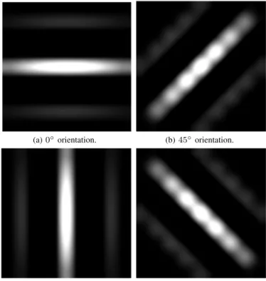
We use the Gabor wavelet feature extraction technique similar to the one used by Reddy et al [26] in their work. Gabor wavelets are a frequency decomposition method similar to Fourier analysis, but instead of decomposing the frequencies in the global manner Gabor wavelets do it in a localised manner. Here the local spectrum is established through (intermediate) features that are obtained by filtering the input image with a set of two-dimensional (2D) Gabor filters [31]. The convolution kernel of a Gabor wavelet is obtained by multiplying a Gaus-sian kernel with a cosine function. Here the Gabor wavelets have two properties to analyse the texture features. The first property is the orientation of the wavelet and the second is the spatial frequency. Further variance of the Gaussian function can be used to fine tune the localisation property of the Gabor wavelet.

The Gabor function is given below,

ψ(x, y, ω0, θ) =√ω0

2πke −ω20

8k2(4(xcosθ+ysinθ)2+(−xsinθ+ycosθ)2) .ei(ω0xcosθ+ω0ysinθ)

(1) where:

ω0=2_λπ and k=π

Here (x,y) is the element location,θ is the orientation and

λ is the wavelength. Elements of the kernel matrix are the real part of the function ψ(x, y, ω₀, θ) and we have chosen the kernel size as 9×9 andλ= 3

Gabor kernels with four different orientations, 0◦_,₄₅◦_,₉₀◦_,₁₃₅◦ _{in the spatial domain are shown in}

Figure 1.

Gabor filters of of these four different orientations (see Figure 1) are applied to the image to extract the image texture features.

In addition to the above features other features such as: 1) Location features

The center coordinate of the spatial block or the spatio temporal cuboid.

2) Motion information. This is the summation of optical flow vectors inside a block [28]. To calculate the the optical flow vectors, we have used Black and Anandan’s algorithm [5].The motion features across a blockB are given by,

(a)0◦orientation. (b)45◦orientation.

(c)90◦orientation. (d)135◦orientation.

Fig. 1: Images of Gabor wavelets in spatial domain of different orientations. σu= (x,y)∈B u(x, y), (2) σv= (x,y)∈B v(x, y). (3) 3) Textures of optical flow [28]

This feature measures the uniformity of the motion, is computed from the dot product of flow vectors at dif-ferent offsets. Uniformity computed at difdif-ferent offsets is useful for detecting objects of various sizes [28]. 4) Image textures [26]

Gabor filters of all four orientations are applied to images as outlined above. This procedure generates a four dimensional feature vector.

These features are evaluated with the learning models outline in Section III. The following feature combinations are evaluated:

Following feature combinations are evaluated 1) Optical flow vector only.

f = [σu, σv]. (4) 2) Optical flow and location.

f = [σu, σv, x, y]. (5) 3) Optical flow, location and textures of optical flow (ToF)

(5)

(a) Van is closer to the camera (b) Van is distant from the camera

Fig. 2: Optical flow variation with scene depth due to perspec-tive distortion.

f =σu, σv, x, y, φ(1,1,0), φ(3,3,0), φ(5,5,0), (6)

whereφ₍_δ,δ,₀₎is uniformity feature value atδoffset [28]. 4) Optical flow, location, ToF at various scales {φ} and image textures at different orientations {α} as given in equation 7.

f = [σu, σv, x, y, φ(1,1,0), φ(3,3,0),φ(5,5,0),

α0, α45, α90, α135],

(7) whereφ₍_δ,δ,₀₎is uniformity feature value atδoffset [28] and α_θ is image texture feature value at θ degrees of orientation.

V. PERSPECTIVENORMALIZATION

Due to the perspective distortion in a scene, objects near to the camera appear to be large while distant objects appear to be small. This can significantly affect the feature extraction methods as the extracted features will vary according to their depth in the scene. Figure 2 shows the variation in the optical flow for the same van at two different depths.

In works related to crowd counting, perspective normaliza-tion has been applied extensively [20, 12, 8, 7, 29]. In these approaches, depth maps were created and features such as areas and edges are scaled appropriately to compensate for distortion due to perspective variation.

To create depth maps for a scene, a number of approaches have been used. Firstly, an infra-red sensor attached to the camera can be used to determine the depth values of objects in the scene [33]. Another approach to use stereo images of an object to estimate the depth information of an object in the scene [10]. However, as most of the publicly available datasets are monocular videos with no other information about the camera parameters, the only available solution is to use geometric correction to remove perspective distortion.

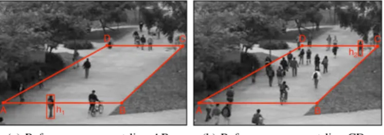
In our work we apply the geometric correction used in [7] and other crowd counting approaches. Here it is assumed that object size varies linearly with they coordinate of the image. A perspective map is approximated by linearly interpolating an object’s size between the two extremes of the scene [7]. As depicted in Figure 3, a rectangular pathway which is lying on the ground is marked and both the width of the pathway and the height of a pedestrian are measured at two locations in the scene. Based on these manual annotations, the width of

(a) Reference person at line AB. (b) Reference person at line CD.

Fig. 3: Geometric correction for perspective distortion. Images from [7].

the pathway w(y) and the height of the pedestrian h(y) are approximated by a linear function of the y coordinate. The perspective map,S(y), assigns a weight to each pixel in row

y as follows:

S(y) = _h₍h_y1₎w_w1₍_y₎ (8) where w₁ and h₁ denote fixed references (at line AB in Figure 4). Thus the perspective map assigns larger weights to smaller objects in the distant parts of the scene.

We weight raw optical flow byS(y)to compensate for the perspective distortion. The other features (location, textures of optical flow and image texture) are used without any change.

VI. EXPERIMENTALRESULTS

In this work we have tested new feature combinations with different modelling techniques [24, 28], and other existing feature combinations as outlined in Section IV. In addition, we evaluate the effect of applying perspective normalization on the publicly available UCSD datasets [21]. This video dataset contains bi-directional pedestrian traffic from two camera view points. Several video sequences (each of 200 frames duration) which contain normal pedestrian movements are used for the training. The testing video sequences contain abnormalities, such as the presence of abnormal objects, anomalous pedes-trian motions and spatial abnormalities, and are annotated with frame-level ground truth.

Perspective normalization is applied to different feature combinations and modelled using different learning models. Table I and II show the results for the Peds1 and Peds2 datasets respectively for these combinations of features with different models (the best performing feature vector for each learning model is shown in bold, and the best performing feature vector and learning model combination in each dataset is underlined). It can be seen that the Ped1 dataset gave best results with perspective normalization as most of the motion relating to the objects in the scene happens perpendicular to the camera plane, while the Ped2 dataset shows little improvement with perspective normalization as objects in the scene move in parallel to the camera plane.

For the Ped1 dataset, modelling only the optical flow features significantly improves with the perspective normaliza-tion. Previously without perspective normalization including the location feature allowed a system to compensate for the

(6)

GMM X-HMM Y-HMM

Without PN With PN Without PN With PN Without PN With PN

Feature Combinations EER AUC EER AUC EER AUC EER AUC EER AUC EER AUC

OF 32.07% 0.754 26.46% 0.819 31.30% 0.750 19.93% 0.878 29.09% 0.783 21.26% 0.868

OF, Location 24.36% 0.839 22.86% 0.850 26.01% 0.814 22.96% 0.854 21.83% 0.859 20.65% 0.854 OF, ToF, Location 23.94% 0.828 20.69% 0.866 29.71% 0.767 22.86% 0.857 26.14% 0.796 22.13% 0.860 OF, ToF, IT, Location 28.06% 0.783 24.19% 0.822 28.82% 0.779 26.31% 0.826 22.89% 0.833 22.03% 0.855

TABLE I: Comparison of performances of different feature combinations with different models on Peds1dataset: PN stands for perspective normalization, ToF stands for Textures of Optical Flow [28], IT stands for Image Textures, O/F stands for Optical Flow based features, EER stands for Equal Error Rate and AUC stands for Area Under Curve.

GMM X-HMM Y-HMM

Without PN With PN Without PN With PN Without PN With PN

Feature Combinations EER AUC EER AUC EER AUC EER AUC EER AUC EER AUC

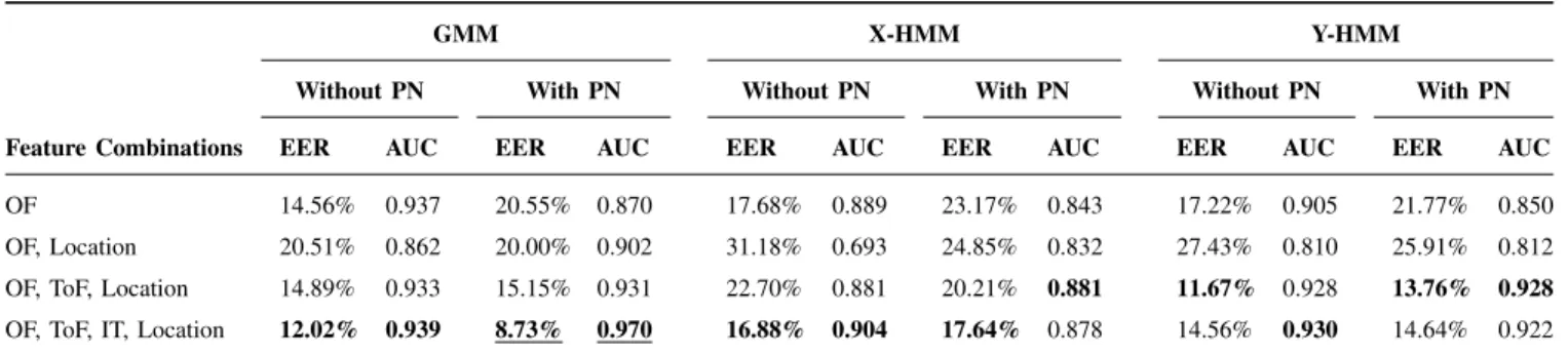
OF 14.56% 0.937 20.55% 0.870 17.68% 0.889 23.17% 0.843 17.22% 0.905 21.77% 0.850 OF, Location 20.51% 0.862 20.00% 0.902 31.18% 0.693 24.85% 0.832 27.43% 0.810 25.91% 0.812 OF, ToF, Location 14.89% 0.933 15.15% 0.931 22.70% 0.881 20.21% 0.881 11.67% 0.928 13.76% 0.928

OF, ToF, IT, Location 12.02% 0.939 8.73% 0.970 16.88% 0.904 17.64% 0.878 14.56% 0.930 14.64% 0.922

TABLE II: Comparison of performances of different feature combinations with different models on Peds2 dataset. The same notation as Table I is used here.

perspective distortion to some extent. Without location features results are poor, but once the optical flow features are per-spective normalized, results significantly improve with all the models. Other feature combinations also show improvements. The GMM gives best result for the perspective normalized feature combination of textures of optical flow, optical flow and location while the X-HMM and Y-HMM give best results for the perspectively normalized feature combination of optical flow only and optical flow with location respectively. Figures 5a, 6a, 7a show ROC curves for the different feature com-binations with different models and the improvements with the perspective normalization can be seen. Figures 4a and 4c show failures to detect the presence of a skateboarder and couple of bicycles in the far field of the camera without perspective normalization, whereas Figures 4b and 4d show that with the application of perspective normalization these distant abnormal objects can be detected.

For the Ped2 dataset Gabor wavelets for image textures are applied and the extracted 4 dimensional feature vector (differ-ent ori(differ-entations) is combined with the other optimum feature combinations [28] to achieve improvement in the results. After applying the perspective normalization the best result is achieved, allowing events such as the slow moving bicycle (see Figure 4f) to be detected for a longer duration. Here, it can be observed that with the perspective normalization the GMM performs well while the performance of the Y-HMM is better without the perspective normalization, and X-HMM

performs poorly compared to the other models in both cases. Figures 5b, 6b, 7b show the ROC curves for the different feature combinations with different models. Figures 4e and 4g show the failures to detect the slow moving bicycle and the presence of a partially occluded bicycle and skateboarder, while Figures 4f and 4h show that the addition of image textures to the previous combination enables the respective detections.

Regarding the models, it can be seen that X-HMM and Y-HMM perform best with a single feature (optical flow) for Ped1, but perform best with a more complex feature vector for Ped2. This is mainly because most of the anomalies in Ped1 can be detected with only motion information, including the abnormal objects such as vehicles and bicycles as their speed is significantly high compared to the normal walking pedestrians; whereas as in Ped2 abnormal events include slow moving bicycles which move at approximately the same speed as pedestrians. Hence the combination of multiple features with motion features performs well for Ped2. Further it can be seen that the GMM performs best with the inclusion of image textures while the X-HMM and Y-HMM performance degrades when these features are included. This is due to the possibility of the background being modelled with the image textures in the case of the X-HMM and Y-HMM, as their feature vectors are spanning a larger area in the spatial domain by taking in to account observations from the adjacent spatial locations. The models (and particularly the HMMs) are limited

(7)

(a) Skateboarder at very distance is not detected without PN

(b) Skateboarder at very distance is detected with PN

(c) Couple of bicycles at very distance is not detected without PN

(d) Couple of bicycles at very distance is detected with PN.

(e) Slow moving bicycle is not detected without image textures

(f) Slow moving bicycle is detected with image textures.

(g) Bicycle and skate border are not detected without image textures

(h) Bicycle and skate border are detect-ed with image textures

Fig. 4: Representative frames demonstrating the proposed anomaly detection algorithm. The left column is without the proposed techniques and the right column is with the proposed techniques [21], PN stands for Perspective Normalization

by the amount of data available. Hence lack of training data degrades the performance when additional features such as location are added to the HMM systems with a high number of states, which is especially the case for Ped1.

Overall, Table I shows that perspective normalization im-proves performance in every experiment on Ped1 except in a single case, while Table II shows that it has no major effect on Ped2 because perspective plays no significant role in that scene. Furthermore, the addition of the image textures feature to the state of the art feature combination of [28] achieves the best results for the Ped2 dataset.

Regarding the speed of the models, on average it takes 0.09 sec to process a frame (11 fps) for all three models on a computer with a 2.53 GHz Intel i5 processor and 4

0 0.1 0.2 0.3 0.4 0.5 0.6 0.7 0.8 0.9 1 0 0.1 0.2 0.3 0.4 0.5 0.6 0.7 0.8 0.9 1

False positive rate

True positive rate

Results for the UCSD Peds1 database for GMM

O/F without PN O/F with PN

O/F and Location without PN O/F and Location with PN O/F, ToF and Location without PN O/F, ToF and Location with PN O/F, ToF, IT and Location without PN O/F, ToF, IT and Location with PN

(a) ROC curves of Ped1 of different feature combinations with GMM.

0 0.1 0.2 0.3 0.4 0.5 0.6 0.7 0.8 0.9 1 0 0.1 0.2 0.3 0.4 0.5 0.6 0.7 0.8 0.9 1

False positive rate

True positive rate

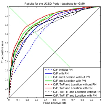
Results for the UCSD Peds2 database for GMM

(b) ROC curves of Ped2 of different feature combinations with GMM.

Fig. 5: ROC curves of Ped1 and Ped2 of different feature combinations with GMM

GB memory, running in a single threaded configuration. Both versions of the Semi-2D HMM require significantly more memory compared to the GMM approach.

VII. CONCLUSION ANDFUTUREWORK

We have evaluated different feature combinations applied to a variety of learning models. Perspective normalization was applied to compensate for the perspective distortion. It can be seen that the application of perspective normalization improves performance on scenes where the effects of perspective are strong. Optical flow features modelled by the Semi-2D

(8)

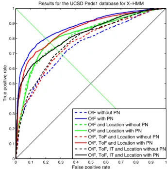
X-0 0.1 0.2 0.3 0.4 0.5 0.6 0.7 0.8 0.9 1 0 0.1 0.2 0.3 0.4 0.5 0.6 0.7 0.8 0.9 1

False positive rate

True positive rate

Results for the UCSD Peds1 database for Y−HMM

(a) ROC curves of Ped1 of different feature combinations with Y-HMM.

0 0.1 0.2 0.3 0.4 0.5 0.6 0.7 0.8 0.9 1 0 0.1 0.2 0.3 0.4 0.5 0.6 0.7 0.8 0.9 1

False positive rate

True positive rate

Results for the UCSD Peds2 database for Y−HMM

(b) ROC curves of Ped2 of different feature combinations with Y-HMM.

Fig. 6: ROC curves of Ped1 and Ped2 of different feature combinations with Y-HMM

HMM [24] yielded the best EER of 19.91%, compared to other state of the art works [24]. For the Ped2 dataset, the combi-nation of optical flow, textures of optical flow [28], image textures using Gabor wavelets and location with perspective normalization gave best EER of 8.44% compared to other state of the art works [24]. It was observed that the addition of image textures using Gabor wavelets doesn’t work as well for the Ped1 dataset, as some background objects such as waving trees are also included in the model captured by the image textures. 0 0.1 0.2 0.3 0.4 0.5 0.6 0.7 0.8 0.9 1 0 0.1 0.2 0.3 0.4 0.5 0.6 0.7 0.8 0.9 1

False positive rate

True positive rate

Results for the UCSD Peds1 database for X−HMM

(a) ROC curves of Ped1 of different feature combinations with X-HMM. 0 0.1 0.2 0.3 0.4 0.5 0.6 0.7 0.8 0.9 1 0 0.1 0.2 0.3 0.4 0.5 0.6 0.7 0.8 0.9 1

False positive rate

True positive rate

Results for the UCSD Peds2 database for X−HMM

(b) ROC curves of Ped2 of different feature combinations with X-HMM.

Fig. 7: ROC curves of Ped1 and Ped2 of different feature combinations with X-HMM

Future works will be seek to extend this evaluation to other databases, features and learning models. Based on these results, approaches which can perform effectively over a variety of conditions will be developed.

REFERENCES

[1] A. Adam, E. Rivlin, I. Shimshoni, and D. Reinitz, “Robust realtime unusual event detection using multiple fixed-location monitors,” inIEEE Trans. Pattern Anal. Mach. Intell, vol. 30, no. 3, Mar 2008, pp. 555–560. [2] E. Andrade, S. Blunsden, and R. Fisher, “Hidden markov models for

(9)

[3] ——, “Modelling crowd scenes for event detection,” in ICPR, vol. 1, 2006, p. 4.

[4] Y. Benezeth, P. Jodoin, V. Saligrama, and C. Rosenberger, “Abnormal events detection based on spatio-temporal co-occurrences,,” in IEEE Conf. Comput. Vision Pattern Recog.Workshops, Jun.2025 2009, pp. 2458–2465.

[5] M. J. Black and P. Anandan, “The robust estimation of multiple motions: parametric and piecewise-smooth flow fields.” inComput. Vis. Image Underst, 1996.

[6] G. R. Bradski and J. W. Davis, “Motion segmentation and pose recog-nition with motion history gradients,,” inMach. Vision Appl, vol. 13, no. 3, 2002, pp. 174–184.

[7] A. B. Chan, Z.-S. J. Liang, and N. Vasconcelos, “Privacy preserving crowd monitoring: Counting people without people models or tracking,” inCVPR, 2008.

[8] A. B. Chan and N. Vasconcelos, “Counting people with low-level features and bayesian regression,” in IEEE Transactions on Image Processing, 2012.

[9] Y. Chen, G. Liang, K. K. Lee, and Y. Xu, “Abnormal behavior detection by multi-svm-based bayesian network,” inInt. Conf. Inf. Acquisition, 2007, pp. 298–303.

[10] L. Falkenhagen, “Depth estimation from stereoscopic image pairs assum-ing piecewise continuos surfaces,” inImage Processing for Broadcast and Video Production, 1994.

[11] T. Hospedales, S. Gong, and T. Xiang, “A markov clustering topicmodel for mining behaviour in video,” inIEEE 12th Int. Conf. Comput. Vision, 2009, pp. 1165–1172.

[12] Y.-L. Hou and G. Pang, “People counting and human detection in a challenging situation,” inSystems, Man and Cybernetics, Part A: Systems and Humans, IEEE Transactions, 2011.

[13] W. Hu, X. Xiao, Z. Fu, D. Xie, T. Tan, and S. Maybank, “A system for learning statistical motion patterns,” inIEEE Trans. Pattern Anal. Mach. Intell, vol. 28, no. 9, Sep 2006, pp. 1450–1464.

[14] J. Kim and K. Grauman, “Observe locally, infer globally: A space-time mrf for detecting abnormal activities with incremental updates,” inIEEE Conf. Comput. Vision Pattern Recog, 2009, pp. 2921–2928.

[15] L. Kratz and K. Nishino, “Anomaly detection in extremely crowded scenes using spatio-temporal motion pattern models,” inIEEE Conf. Comput. Vision Pattern Recog, 2009, pp. 1446–1453.

[16] C. K. Lee, M. F. Ho, W. S. Wen, and C. L. Huang, “Abnormal event detection in video using n-cut clustering,” inInt. Conf. Intell. Inf. Hiding Multimedia Signal Process, 2006, pp. 407–410.

[17] T. S. Lee, “Image representation using 2d gabor wavelets,” Pattern Analysis and Machine Intelligence, IEEE Transactions, vol. 18, pp. 959 – 971, 1996.

[18] H. Li, Z. Hu, Y. Wu, and F. Wu, “Behavior modeling and abnormality detection based on semi-supervised learning method,” inRuan Jian Xue Bao/J. Software, vol. 18, 2007., pp. 527–537,.

[19] J. Li, T. M. Hospedales, S. Gong, and T. Xiang, “Learning rare behaviours,,” in10th Asian Conf. Computer Vision, 2010, pp. 293–307. [20] R. Ma, L. Li, W. Huang, and Q. Tian, “On pixel count based crowd density estimation for visual surveillance,” inIn IEEE Conference on Cybernetics and Intelligent Systems, 2004, 2005.

[21] V. Mahadevan, W. Li, V. Bhalodia, and N. Vasconcelos, “Anoma-ly detection in crowded scenes,” in Computer Vision and Pattern Recognition, 2010 IEEE Conference, jun 2010, pp. 1975–1981,, http://www.svcl.ucsd.edu/projects/anomaly/.

[22] R. Mehran, A. Oyama, and M. Shah, “Abnormal crowd behavior detection using social force model,” in IEEE Conf. Computer Vision Pattern Recog, 2009, pp. 935–942.

[23] B. T. Morris, “Trajectory learning for activity understanding : Unsuper-vised, multilevel, and long-term adaptive approach.” inIEEE Transac-tions on Pattern Analysis and Machine Intelligence., 2011.

[24] H. Nallaivarothayan, D. Ryan, S. Denman, S. Sridharan, and C. Fookes, “Anomalous event detection using a semi-two dimensional hidden markov model,” inDigital Image Computing Techniques and Applica-tions (DICTA), 2012 International Conference, 2012, pp. 1 – 7. [25] O. P. Popoola and K. Wang, “Video-based abnormal human behavior

recognitiona review,” inIEEE TRANSACTIONS ON SYSTEMS, MAN, AND CYBERNETICSPART C: APPLICATIONS AND REVIEWS, 2011. [26] V. Reddy, C. Sanderson, and B. C. Lovell, “Improved anomaly detection in crowded scenes via cell-based analysis of foreground speed, size and texture,” inIEEE Comput. Soc. Conf. Comput. Vision Pattern Recog. Workshops, 2011, pp. 55–61.

[27] C. Rougier, J. Meunier, A. St-Arnaud, and J. Rousseau, “Fall detection from human shape and motion history using video surveillance,,” in21st Int. Conf. Adv. Inf. Netw. Appl. Workshops, 2007, pp. 875–880. [28] D. Ryan, S. Denman, C. Fookes, and S. Sridharan, “Textures of optical

flow for real-time anomaly detection in crowds,” in8th IEEE Int. Conf. Adv. Video Signal Based Surveillance, 2011, pp. 230–235.

[29] D. Ryan, S. Denman, S. Sridharan, and C. Fookes, Scene invariant crowd counting and crowd occupancy analysis. Springer-Verlag, Germany, 2012, ch. Video Analytics for Business Intelligence [Studies in Computational Intelligence, Volume 409], pp. 161–198.

[30] G. Schwarz, “Estimating the dimension of a model,”The An-nals of Statistics, vol. 6, p. 461464, 1978.

[31] G. S.E, P. N, and K. P, “Comparison of texture features based on gabor filters,”Image Processing, IEEE Transactions on, vol. 11, pp. 1160 – 1167, 2002.

[32] J. Snoek, J. Hoey, L. Stewart, and R. S. Zemel, “Automated detection of unusual events on stairs,” in3rd Canadian Conf. Comput. Robot Vision, 2006, p. 5.

[33] E. Stone and M. Skubic, “Evaluation of an inexpensive depth camera for passive in-home fall risk assessment,” in Pervasive Computing Technologies for Healthcare (PervasiveHealth), 2011 5th International Conference on, 2011.

[34] X. Wu, Y. Ou, H. Qian, and Y. Xu, “A detection system for human abnormal behavior,” in IEEE/RSJ Int. Conf. Intell. Robots Syst, 2005, pp. 1204–1208.

[35] T. Xiang and S. Gong, “Incremental and adaptive abnormal behaviour detection .” inComput. Vis. Image Understanding,, vol. 111, 2008, pp. 59–73,.

[36] T. XIANG and S. GONG, “Beyond tracking : Modelling activity and understanding behaviour,” inInternational Journal of Computer Vision, 2006.

[37] X. Zhang, H. Liu, Y. Gao, and D. H. Hu, “Detecting abnormal events via hierarchical dirichlet processes,” in13th Pacific-Asia Conf. Knowledge Discovery Data Mining, Apr.2730 2009, pp. 278–289.

[38] B. Zhao and E. P.Xing, “Online detection of unusual events in videos via dynamic sparse coding,” inCVPR11, 2011, pp. 3313–3320. [39] H. Zhou and D.Kimber, “Unusual event detection via multi-camera video

mining,” in18th Int. Conf. Pattern Recog, 2006, pp. 1161–1166. [40] X. Zou and B. Bhanu, “Anomalous activity classification in the

distribut-ed camera network,” in15th IEEE Int. Conf. Image Process, 2008, pp. 781–784.