Selection of our books indexed in the Book Citation Index in Web of Science™ Core Collection (BKCI)
Interested in publishing with us?
Contact [email protected]
Numbers displayed above are based on latest data collected.For more information visit www.intechopen.com Open access books available
Countries delivered to Contributors from top 500 universities
International authors and editors
Our authors are among the
most cited scientists
Downloads
We are IntechOpen,
the world’s leading publisher of
Open Access books
Built by scientists, for scientists
12.2%
122,000
135M
TOP 1%
154
A New Non-dominated Sorting Genetic Algorithm for Multi-Objective
Optimization
Chih-Hao Lin and Pei-Ling Lin
X
A New Non-dominated Sorting Genetic
Algorithm for Multi-Objective Optimization
Chih-Hao Lin and Pei-Ling Lin
Department of Information Management, Chung Yuan Christian University
Taiwan, R.O.C.
1. Introduction
Multi-objective optimization (MO) is a highly demanding research topic because many real-world optimization problems consist of contradictory criteria or objectives. Considering these competing objectives concurrently, a multi-objective optimization problem (MOP) can be formulated as finding the best possible solutions that satisfy these objectives under different tradeoff situations. A family of solutions in the feasible solution space forms a Pareto-optimal front, which describes the tradeoff among several contradictory objectives of an MOP. Generally, there are two goals in finding the Pareto-optimal front of a MOP: 1) to converge solutions as near as possible to the Pareto-optimal front; and 2) to distribute solutions as diverse as possible over the obtained non-dominated front. These two goals cause enormous search space in MOPs and let deterministic algorithms feel difficult to obtain the Pareto-optimal solutions. Therefore, satisfying these two goals simultaneously is a principal challenge for any algorithm to deal with MOPs (Dias & Vasconcelos, 2002). In recent years, several evolutionary algorithms (EAs) have been proposed to solve MOPs. For example, the strength Pareto evolutionary algorithm (SPEA) (Zitzler et al., 2000) and the revised non-dominated sorting genetic algorithm (NSGA-II) (Deb et al., 2002) are two most famous algorithms. Several extensions of genetic algorithms (GAs) for dealing with MOPs are also proposed, such as the niche Pareto genetic algorithm (NPGA) (Horn et al., 1994), the chaos-genetic algorithm (CGA) (Qi et al., 2006), and the real jumping gene genetic algorithm (RJGGA) (Ripon et al., 2007).
However, most existing GAs only evaluate each chromosome by its fitness value regardless of the schema structure, which is a gene pattern defined by fixing the values of specific gene loci within a chromosome. The schemata theorem proved by Goldberg in 1989 is a central result of GA’s theory in which a larger of effective genomes implies a more efficient of searching ability for a GA (Goldberg, 1989).
Inspired by the outstanding literature of Kalyanmoy Deb, this study proposes an evaluative crossover operator to incorporate with the original NSGA-II. The proposed evaluative version of NSGA-II, named E-NSGA-II, can further enhance the advantages of the fast non-dominated sorting and the diversity preservation of the NSGA-II for improving the quality of the Pareto-optimal solutions in MOPs. The proposed evaluative crossover imitates the therapy process at the forefront of medicine and therefore integrates a new
evaluation method with a gene-therapy approach in the traditional uniform crossover scheme. The gene-evaluation method evaluates the merit of different genes between two mating parents by mutually exchanging these therapeutic genes one-by-one and observing the fitness variances. And then, the proposed evaluative crossover adopts a gene-therapy approach to cure the mating parents mutually with respect to their gene contribution to retain superior genomes in the evolutionary population.
The particular advantage of E-NSGA-II is that the gene-evaluation method can implicitly generate effective genome without explicitly analyzing the solution space by classical local search techniques. The performance of the proposed algorithm is experimented on nine unconstrained benchmark MOPs. The experiment results show that the E-NSGA-II not only can converge the nondominated solutions to the Pareto-optimal front but also can enhance the solution diversity to spread the achieved extent for all test MOPs.
The rest of this chapter is organized as follows. Section 2 introduces the genetic operators of the proposed E-NSGA-II. Section 3 describes numerical implementation and parameter setting. Section 4 reports the computational experiments on unconstrained MOPs and discusses the characteristics of E-NSGA-II. Finally, this chapter concludes with a summary in Section 5.
2. Algorithm Description
The NSGA proposed by Srinivas and Deb (1994) is one of the first EAs for MOPs (Srinivas & Deb, 1994). The main idea of the NSGA is the ranking process executed before the selection operation. In 2002, Deb et al. proposed a revised version, named NSGA-II, by introducing fast non-dominated sorting and diversity preservation policies (Deb et al., 2002). Three features of NSGA-II are summarized as follows:
1) Computational complexity: NSGA-II uses a fast non-dominated sorting approach to substitute for the original sorting algorithm of NSGA in order to reduce its computational complexity from O(MP3) to O(MP2), where M is the number of objectives and P is the
population size. This feature makes NSGA-II more efficient than NSGA for large population cases.
2) Elitism preservation: Replacement-with-elitism methods can monotonously enhance the solution quality and speed up the performance of GAs significantly (Ghomsheh et al., 2007). NSGA-II adopts (μ+λ)-evolution strategy to keep elitism solutions and prevent the loss of good solutions once they are found. Successive population is produced by selecting μ better solutions from μ parents and λ children.
3) Parameter reduction: Traditional sharing approach is a diversity ensuring mechanism that can get a wide variety of equivalent solutions in a population. However, a sharing parameter should be specified to set the sharing extent desired in a problem. Therefore, NSGA-II defines a density-estimation metric and applies the crowded-comparison operator with less required parameters to keep diversity between solutions.
In this study, the proposed E-NSGA-II stems from a concept different from traditional NSGA-II, particularly in terms of the gene-evaluation method. That is, the E-NSGA-II inherits the advantages of the NSGA-II and emphasizes the development of a new crossover operator and a modified replacement policy (Lin & Chuang, 2007).
2.1 Generation of Initial Population
A real coding representation is efficiently applied to solve numerical MOPs. Each test MOP is structured in the same manner and consists of M objective functions (Deb, 1999):
( ), , ( )
) ( Minimize T x f1 x fM x (1)
T n x x x x , , , where 1 2 . (2)Each decision variable is treated as a gene and encoded by a floating-point number. Each chromosome representing a feasible solution is encoded as a vector T n
n x x x x[ 1 2 ] ,
where xi denotes the value of the ith gene and n is the number of design variables in an MOP. Because the lower bound T
n l l l l [1 2 ]
and the upper bound T
n
u u u
u[ 1 2 ] define
the feasible solution space, the domain of each xi is denoted as interval [li, ui].
The main components of the E-NSGA-II are chromosome encoding, fitness function, selection, recombination and replacement. An initial population with P chromosomes is randomly generated within the predefined feasible region. At each generation, E-NSGA-II applies the fast non-dominated sorting of NSGA-II to identify non-dominated solutions and construct the non-dominated front. And then, E-NSGA-II executes the rank comparison in selection operation to decide successive population by elitism strategy as the diversity preservation in NSGA-II (Deb et al., 2002). Therefore, the following sections only describe the details of the evaluative crossover operator and the diverse replacement.
2.2 Evaluative Crossover
For evaluation purpose, this study applies the crowding distance as an evaluation of chromosome’s quality in the evaluative crossover. The crowding distance proposed in NSGA-II is used to estimate the density quantity of a particular solution in the population by calculating the average distance between other surrounding solutions with respect to each objective (Deb et al., 2002).After two parents have been selected from population, let the parent with larger crowding distance be named as the better parent (xb) and the other one is the worse parent (xw). Their crossover child is denoted as
y
.The proposed evaluative crossover imitates the gene-therapy process at the forefront of medicine, which inserts genes into an individual's cells to treat a disease by replacing a defective mutant allele by a functional one. Therefore, the evaluative crossover integrates a gene-evaluation method with a gene-therapy approach in the traditional uniform crossover scheme. By randomly generating a therapeutic mask with the same length as chromosomes, each parity bit in the therapeutic mask indicates whether the gene locus should be cured or not. For each gene locus, a random number in the interval [0, 1] is generated and compared to a pre-defined crossover rate pc. If the random number is larger than the crossover rate, the parity bit in the therapeutic mask is assigned as 0 and no crossover occurs at this locus (iGc). Otherwise, the parity bit in the therapeutic mask is assigned as 1 and the child’s gene is generated by the gene-therapy approach (iGc).
Firstly, the gene-evaluation method mutually exchanges two parity genes between two mating parents and then compares their fitness variance as a measurement of these genes’ merit. The exclusive features of the gene-evaluation method include that 1) the contribution
of each gene is evaluated individually; and 2) the gene merit is estimated by the improvement of their density quantity during the gene-swap process (Lin & He, 2007). Secondly, one temporary chromosome is generated for crossover locus i, denoted as
T bn i b i b b i x x x xt 1,, (1),xwi, (1),, . This temporary chromosome clones all alleles in the better
parent and then replaces the selected gene of the better parent (xbi) with the one of the worse parent (xwi) in the same locus. The contribution of the gene xwi is denoted as dwi and approximated by the Euclidean distance between ti and xw by Equation (3). For comparison purpose, the Euclidean distance between xb and xw calculating by Equation (4) is the contribution of the gene xbi and denoted as dbi. Therefore, comparing dbi with dwi can reveal the contributions of xbi and xwi with respect to the genetic material of the better parent.
M m m i m w w i wi dist t x f t f x d 1 2 ) ( ) ( ) , ( (3)
M m m b m w w b bi dist x x f x f x d 1 2 ) ( ) ( ) , ( (4)Finally, the gene-therapy approach can cure some defective genes in the better parent (i.e. xbi) according to the genetic material of the other parent (i.e. xwi) and then produce a child gene (i.e. yi) for the evolutionary process. If the parity bit in the therapeutic mask is 0 (e.g. iGc), the offspring directly inherits the parity gene from the better parent, i.e. the gene in the better parent (xbj) is equal to that in the child (i.e. yj = xbj) at the same locus. On the other hand, if the parity bit in the therapeutic mask is 1 (e.g. iGc), the therapy gene of the child at the same locus (i.e. yj) is arithmetically combined from the parity genes of the mated parents (i.e. xbj and xwj) according to their gene contributions. Each gene in the crossover child can be reproduced by Equation (5) in which coef is a random number in interval [0.5, 1.0].
) ( and ) ( if ) ( and ) ( if ) ( if , ) 1 ( ), 1 ( , wi bi c wi bi c c wi bi wi bi bi i d d G i d d G i G i coef x coef x coef x coef x x y (5)
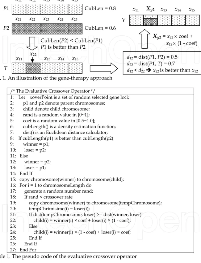
Example: In Fig. 1, the better parent with larger crowding distance (Cub_len = 0.8) is P1 and
the worse parent (Cub_len = 0.6) is P2. The therapy gene is the 2nd gene in chromosomes. The temporary chromosome T clones all of genes in P1 except for the 2nd gene, which copies from x22 in P2. We assume that the Euclidean distance (d12) between P1 and P2 is 0.5
and the distance (d22) between P1 and T is 0.7, which are used to estimate the gene
contribution of x12 and x22, respectively. Because d22 is larger than d12, the 2nd gene in P2 (x22)
is better than that in P1 (x12). Therefore, the child’s gene (xy2) inherits more genetic material
from x22 than x12.The pseudo code of the evaluative crossover is described in Table 1.
2.3 Polynomial Mutation
Mutation operator is applied to enlarge the population diversity to escape from local optima and therefore enhance the exploration ability. E-NSGA-II inherits the polynomial mutation used by NSGA-II and operates as Equation (6) and (7) (Deb & Goyal, 1996).
Fig. 1. An illustration of the gene-therapy approach
/* The Evaluative Crossover Operator */
1: Let xoverPoint is a set of random selected gene loci; 2: p1 and p2 denote parent chromosomes;
3: child denote child chromosome; 4: rand is a random value in [0~1]; 5: coef is a random value in [0.5~1.0];
6: cubLength() is a density estimation function; 7: dist() is an Euclidean distance calculator; 8: If cubLength(p1) is better than cubLength(p2) 9: winner = p1; 10: loser = p2; 11: Else 12: winner = p2; 13: loser = p1; 14: End If
15: copy chromosome(winner) to chromosome(child); 16: For i = 1 to chromosomeLength do
17: generate a random number rand; 18: If rand < crossover rate
19: copy chromosome(winner) to chromosome(tempChromosome); 20: tempChrimisime(i) = loser(i);
21: If dist(tempChromosome, loser) >= dist(winner, loser) 22: child(i) = winner(i) × coef + loser(i) × (1 - coef); 23: Else
24: child(i) = winner(i) × (1 - coef) + loser(i) × coef; 25: End If
26: End If 27: End For
Table 1. The pseudo code of the evaluative crossover operator
i L i u i t i t i x x x y(1,1) (1,1)( ( ) ( )) (6) , )] 1 ( 2 [ 1 , 1 ) 2 ( ) 1 /( 1 ) 1 /( 1 m m i i i r r 5 . 0 5 . 0 i i r if r if (7) x11 x12 x13 x14 x15 P1 P2 CubLen = 0.8 CubLen = 0.6 Y CubLen(P2) < CubLen(P1) P1 is better than P2
X
y2 = x22 coef + x12 (1 - coef) T d12 = dist(P1, P2) = 0.5 d22 = dist(P1, T) = 0.7 d12 < d22x22 is better than x12 x21 x22 x23 x24 x25 x11x
22 x13 x14 x15 x11X
y2 x13 x14 x15of each gene is evaluated individually; and 2) the gene merit is estimated by the improvement of their density quantity during the gene-swap process (Lin & He, 2007). Secondly, one temporary chromosome is generated for crossover locus i, denoted as
T bn i b i b b i x x x xt 1,, (1),xwi, (1),, . This temporary chromosome clones all alleles in the better
parent and then replaces the selected gene of the better parent (xbi) with the one of the worse parent (xwi) in the same locus. The contribution of the gene xwi is denoted as dwi and approximated by the Euclidean distance between ti and xw by Equation (3). For comparison purpose, the Euclidean distance between xb and xw calculating by Equation (4) is the contribution of the gene xbi and denoted as dbi. Therefore, comparing dbi with dwi can reveal the contributions of xbi and xwi with respect to the genetic material of the better parent.
M m m i m w w i wi dist t x f t f x d 1 2 ) ( ) ( ) , ( (3)
M m m b m w w b bi dist x x f x f x d 1 2 ) ( ) ( ) , ( (4)Finally, the gene-therapy approach can cure some defective genes in the better parent (i.e. xbi) according to the genetic material of the other parent (i.e. xwi) and then produce a child gene (i.e. yi) for the evolutionary process. If the parity bit in the therapeutic mask is 0 (e.g. iGc), the offspring directly inherits the parity gene from the better parent, i.e. the gene in the better parent (xbj) is equal to that in the child (i.e. yj = xbj) at the same locus. On the other hand, if the parity bit in the therapeutic mask is 1 (e.g. iGc), the therapy gene of the child at the same locus (i.e. yj) is arithmetically combined from the parity genes of the mated parents (i.e. xbj and xwj) according to their gene contributions. Each gene in the crossover child can be reproduced by Equation (5) in which coef is a random number in interval [0.5, 1.0].
) ( and ) ( if ) ( and ) ( if ) ( if , ) 1 ( ), 1 ( , wi bi c wi bi c c wi bi wi bi bi i d d G i d d G i G i coef x coef x coef x coef x x y (5)
Example: In Fig. 1, the better parent with larger crowding distance (Cub_len = 0.8) is P1 and
the worse parent (Cub_len = 0.6) is P2. The therapy gene is the 2nd gene in chromosomes. The temporary chromosome T clones all of genes in P1 except for the 2nd gene, which copies from x22 in P2. We assume that the Euclidean distance (d12) between P1 and P2 is 0.5
and the distance (d22) between P1 and T is 0.7, which are used to estimate the gene
contribution of x12 and x22, respectively. Because d22 is larger than d12, the 2nd gene in P2 (x22)
is better than that in P1 (x12). Therefore, the child’s gene (xy2) inherits more genetic material
from x22 than x12.The pseudo code of the evaluative crossover is described in Table 1.
2.3 Polynomial Mutation
Mutation operator is applied to enlarge the population diversity to escape from local optima and therefore enhance the exploration ability. E-NSGA-II inherits the polynomial mutation used by NSGA-II and operates as Equation (6) and (7) (Deb & Goyal, 1996).
Fig. 1. An illustration of the gene-therapy approach
/* The Evaluative Crossover Operator */
1: Let xoverPoint is a set of random selected gene loci; 2: p1 and p2 denote parent chromosomes;
3: child denote child chromosome; 4: rand is a random value in [0~1]; 5: coef is a random value in [0.5~1.0];
6: cubLength() is a density estimation function; 7: dist() is an Euclidean distance calculator; 8: If cubLength(p1) is better than cubLength(p2) 9: winner = p1; 10: loser = p2; 11: Else 12: winner = p2; 13: loser = p1; 14: End If
15: copy chromosome(winner) to chromosome(child); 16: For i = 1 to chromosomeLength do
17: generate a random number rand; 18: If rand < crossover rate
19: copy chromosome(winner) to chromosome(tempChromosome); 20: tempChrimisime(i) = loser(i);
21: If dist(tempChromosome, loser) >= dist(winner, loser) 22: child(i) = winner(i) × coef + loser(i) × (1 - coef); 23: Else
24: child(i) = winner(i) × (1 - coef) + loser(i) × coef; 25: End If
26: End If 27: End For
Table 1. The pseudo code of the evaluative crossover operator
i L i u i t i t i x x x y(1,1) (1,1)( ( ) ( )) (6) , )] 1 ( 2 [ 1 , 1 ) 2 ( ) 1 /( 1 ) 1 /( 1 m m i i i r r 5 . 0 5 . 0 i i r if r if (7) x11 x12 x13 x14 x15 P1 P2 CubLen = 0.8 CubLen = 0.6 Y CubLen(P2) < CubLen(P1) P1 is better than P2
X
y2 = x22 coef + x12 (1 - coef) T d12 = dist(P1, P2) = 0.5 d22 = dist(P1, T) = 0.7 d12 < d22x22 is better than x12 x21 x22 x23 x24 x25 x11x
22 x13 x14 x15 x11X
y2 x13 x14 x15In Equation (6),
x
i(u)andx
i(L) are the upper and lower bounds of the mutation parameter. According to Deb’s research, the shape of the probability distribution is directly controlled by an external parameter ηm and the distribution is not dynamically changed with generations (Deb, 2001). Therefore, parameter ηm is also fixed in this study.2.4 Diverse Replacement
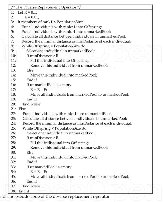
E-NSGA-II modifies the replacement strategy proposed by Ghomsheh et al. in 2007 to keep diversity and generate successive population (Ghomsheh et al., 2007). The replacement criteria relying on the fast non-dominated sorting and diversity metric can keep those better diversity individuals and provide larger search space for crossover and mutation operators. In this study, a competitive population is generated by combining the parent population and the offspring population. In the competitive population, if the number of individuals with rank=1 is less than the population size, the successive population is firstly filled with the best non-dominated solutions and then selects the highest diversity solutions from the remaining individuals with rank>1 until the pre-specified population size is achieved. On the other hand, the successive population is sequentially filled with the best diversity solution from individuals with rank=1 until the size of the successive population is equal to the population size. According to these replacement criteria, the successive population can be generated. The pseudo code of replacement procedure is described in Table 2.
3. Numerical Implementation
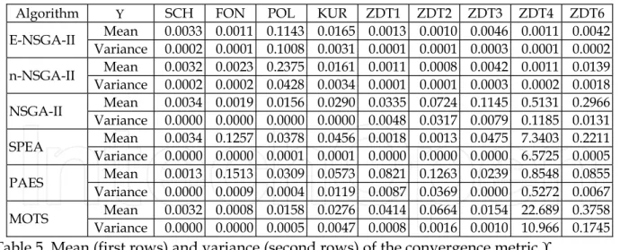
For each test MOP, E-NSGA-II performs 10 runs with different seeds to observe the consistency of the outcome. The mean value of the measures reveals the average evolutionary performance of E-NSGA-II and represents the optimization results in comparison with other algorisms.The variance of the best solutions in 10 runs indicates the consistency of an algorithm. E-NSGA-IIis implemented by MATLAB.
3.1 Performance Measures
Different performance measures for evaluating efficiency have been suggested in literature (Okabe et al., 2003). For comparison purpose, this study applies two metrics: 1) the convergence metric (Υ): approximating the average distance to the Pareto-optimal front; and 2) the diversity metric (Δ): measuring the extent of spread achieved among the obtained solutions (Deb, 2001).
For the convergence metric (Υ), a smaller metric value implies a better convergence toward the Pareto-optimal front. This study uses 500 uniformly spaced solutions to approximate the true Pareto-optimal. To measure the distance between the obtained non-dominated front (Q) and the set of Pareto-optimal solutions (P*), this study computes the minimum Euclidean distance of each solution from 500 chosen points on the Pareto-optimal front by Equation (8). The average of these distances is used as the convergence metric as Equation (9).
Mm k m i m P k i f f d | | 1 *( ) 2 1 ( )min
* (8) Q d Q i i
( 1 ) (9)/* The Diverse Replacement Operator */ 1: Let R = 0.1;
2: E = 0.01;
3: If members of rank1 < PopulationSize
4: Put all individuals with rank=1 into Offspring; 5: Put all individuals with rank>1 into unmarkedPool;
6: Calculate all distance between individuals in unmarkedPool; 7: Record the minimal distance as minDistance of each individual; 8: While Offspring < PopulationSize do
9: Select one individual in unmarkedPool; 10: If minDistance > R
11: Fill this individual into Offspring;
12: Remove this individual from unmarkedPool; 13: Else
14: Move this individual into markedPool; 15: End if
16: If unmarkedPool is empty 17: R = R – E;
18: Move all individuals from markedPool to unmarkedPool; 19: End if
20: End while 21: Else
22: Put all individuals with rank=1 into unmarkedPool;
23: Calculate all distance between individuals in unmarkedPool; 24: Record the minimal distance as minDistance of each individual; 25: While Offspring < PopulationSize do
26: Select one individual in unmarkedPool; 27: If minDistance > R
28: Fill this individual into Offspring;
29: Remove this individual from unmarkedPool; 30: Else
31: Move this individual into markedPool; 32: End if
33: If unmarkedPool is empty 34: R = R – E;
35: Move all individuals from markedPool to unmarkedPool; 36: End if
37: End while 38: End if
Table 2. The pseudo code of the diverse replacement operator
In Equation (8), di is the Euclidean distance between the solution iQ and the nearest member of P*. Indicator k denotes the kth member in P*. Notation M is the number of
objectives and *(k)
m
f is the mth objective function value of kth member in P*. Indicator i in
Equation (9) is the obtained non-dominated solution from E-NSGA-II.
For Diversity metric (Δ), the value of Δ would be close to zero if the non-dominated solutions of the obtained front widely and uniformly spread out. The diversity metric (Δ) measures the extent of spread achieved among the obtained non-dominated solutions and is calculated by Equation (10).
In Equation (6),
x
i(u)andx
i(L) are the upper and lower bounds of the mutation parameter. According to Deb’s research, the shape of the probability distribution is directly controlled by an external parameter ηm and the distribution is not dynamically changed with generations (Deb, 2001). Therefore, parameter ηm is also fixed in this study.2.4 Diverse Replacement
E-NSGA-II modifies the replacement strategy proposed by Ghomsheh et al. in 2007 to keep diversity and generate successive population (Ghomsheh et al., 2007). The replacement criteria relying on the fast non-dominated sorting and diversity metric can keep those better diversity individuals and provide larger search space for crossover and mutation operators. In this study, a competitive population is generated by combining the parent population and the offspring population. In the competitive population, if the number of individuals with rank=1 is less than the population size, the successive population is firstly filled with the best non-dominated solutions and then selects the highest diversity solutions from the remaining individuals with rank>1 until the pre-specified population size is achieved. On the other hand, the successive population is sequentially filled with the best diversity solution from individuals with rank=1 until the size of the successive population is equal to the population size. According to these replacement criteria, the successive population can be generated. The pseudo code of replacement procedure is described in Table 2.
3. Numerical Implementation
For each test MOP, E-NSGA-II performs 10 runs with different seeds to observe the consistency of the outcome. The mean value of the measures reveals the average evolutionary performance of E-NSGA-II and represents the optimization results in comparison with other algorisms.The variance of the best solutions in 10 runs indicates the consistency of an algorithm. E-NSGA-IIis implemented by MATLAB.
3.1 Performance Measures
Different performance measures for evaluating efficiency have been suggested in literature (Okabe et al., 2003). For comparison purpose, this study applies two metrics: 1) the convergence metric (Υ): approximating the average distance to the Pareto-optimal front; and 2) the diversity metric (Δ): measuring the extent of spread achieved among the obtained solutions (Deb, 2001).
For the convergence metric (Υ), a smaller metric value implies a better convergence toward the Pareto-optimal front. This study uses 500 uniformly spaced solutions to approximate the true Pareto-optimal. To measure the distance between the obtained non-dominated front (Q) and the set of Pareto-optimal solutions (P*), this study computes the minimum Euclidean distance of each solution from 500 chosen points on the Pareto-optimal front by Equation (8). The average of these distances is used as the convergence metric as Equation (9).
Mm k m i m P k i f f d | | 1 *( ) 2 1 ( )min
* (8) Q d Q i i
( 1 ) (9)/* The Diverse Replacement Operator */ 1: Let R = 0.1;
2: E = 0.01;
3: If members of rank1 < PopulationSize
4: Put all individuals with rank=1 into Offspring; 5: Put all individuals with rank>1 into unmarkedPool;
6: Calculate all distance between individuals in unmarkedPool; 7: Record the minimal distance as minDistance of each individual; 8: While Offspring < PopulationSize do
9: Select one individual in unmarkedPool; 10: If minDistance > R
11: Fill this individual into Offspring;
12: Remove this individual from unmarkedPool; 13: Else
14: Move this individual into markedPool; 15: End if
16: If unmarkedPool is empty 17: R = R – E;
18: Move all individuals from markedPool to unmarkedPool; 19: End if
20: End while 21: Else
22: Put all individuals with rank=1 into unmarkedPool;
23: Calculate all distance between individuals in unmarkedPool; 24: Record the minimal distance as minDistance of each individual; 25: While Offspring < PopulationSize do
26: Select one individual in unmarkedPool; 27: If minDistance > R
28: Fill this individual into Offspring;
29: Remove this individual from unmarkedPool; 30: Else
31: Move this individual into markedPool; 32: End if
33: If unmarkedPool is empty 34: R = R – E;
35: Move all individuals from markedPool to unmarkedPool; 36: End if
37: End while 38: End if
Table 2. The pseudo code of the diverse replacement operator
In Equation (8), di is the Euclidean distance between the solution iQ and the nearest member of P*. Indicator k denotes the kth member in P*. Notation M is the number of
objectives and *(k)
m
f is the mth objective function value of kth member in P*. Indicator i in
Equation (9) is the obtained non-dominated solution from E-NSGA-II.
For Diversity metric (Δ), the value of Δ would be close to zero if the non-dominated solutions of the obtained front widely and uniformly spread out. The diversity metric (Δ) measures the extent of spread achieved among the obtained non-dominated solutions and is calculated by Equation (10).
0 0.01 0.02 0.03 0.04 0.05 10 20 30 40 50 60 70 80 90 100 Crossover percentage C on ve rg en ce m et ric mean var. 0 0.1 0.2 0.3 0.4 0.5 0.6 10 20 30 40 50 60 70 80 90 100 Crossover percentage D iv er sit y m et ric mean var.
(a)Convergence metric (b) Diversity metric
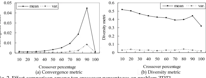
Fig. 2. Effect comparison among ten crossover percentages on problem ZDT1
d N d d d d d d l f N i i l f ) 1 ( 1 1
(10)The Euclidean distances between the extreme solutions of the Pareto front (P*) is df. The
distances between the boundary solutions of the obtained nondominated set (Q) is dl, and the distances between the consecutive solutions in the obtained non-dominated set is di. Notation d is the average of di.
3.2 Parameter Setting
To discover the best configuration for E-NSGA-II, some comprehensive investigations for parameter setting are performed on a benchmark problem. Especially, the performance of the evaluative crossover is influenced by three parameters: 1) crossover percentage; 2) crossover rate; and 3) therapeutic coefficient. The experimental results are averaged in 10 runs and evaluated by the convergence metric and the diversity metric. Problem ZDT1 is selected to analyze the effect of different parameters with a reasonable set of values in these experiments. The test function ZDT1 proposed by Zitzler et al. has a convex Pareto-optimal front and two objective functions without any constraint. The number of decision variables is 30 and the feasible region of each variable is in interval [0, 1].
( ), ( )
) ( Minimize T x f1 x1 f2 x (ZDT1) 1 1 1( ) where f x x (11)
1 / ( )
) ) ( ) ( 1 2 x g x x g x f (12) ) 1 /( ) ( 9 1 ) (x
2x n g in i . (13)1) Effect of Crossover Percentage
The crossover percentage decides how many successive individuals are produced by crossover operator. For example, 80% crossover percentage means that the crossover operator produces 80% offspring and the other 20% are produced by mutation operator. Especially, 100% crossover percentage means that all offspring are firstly recombined by crossover operator and then flipped one or more genes by mutation operator.
0 0.005 0.01 0.015 0.02 0.025 0.03 0.035 1 10 30 50 70 90 Crossover rate C on ve rg en ce m et ric mean var. 0 0.1 0.2 0.3 0.4 0.5 1 10 30 50 70 90 Crossover rate D iv er sit y m et ric mean var.
(a) Convergence metric (b) Diversity metric
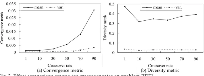
Fig. 3. Effect comparison among ten crossover rates on problem ZDT1
To analyze the best percentage of crossover children in each generation, ten crossover percentages (from 10% to 100%) were tested on problem ZDT1. The mean and variance of the convergence and diversity metrics are depicted in Fig. 2(a) and Fig. 2(b), respectively. In Fig. 2(a), a larger crossover percentage implies a worse convergence situation when the crossover percentage is assigned from 10% to 90%. However, the best convergence is obtained when the crossover percentage is 100%. For diversity metric, Fig. 2(b) shows that the diversity metric is slightly declined from 10% to 70% and then rises until 90%. In particular, the best diversity metric is also obtained when the crossover percentage is 100%. Therefore, all individuals in this study are firstly recombined by the evaluative crossover and then mutated by the polynomial mutation.
2) Effect of Crossover Rate
In the gene-evaluation method, a smaller crossover rate implies a lower computational effort because only the selected loci in the therapeutic mask need to be evaluated individually. To realize the effects of different crossover rates (pc), six simulations with crossover rates from 1% to 90% are conducted on problem ZDT1 to discover the best crossover rate.
The convergence and diversity metrics of experimental results are depicted in Fig. 3(a) and 3(b), respectively. In Fig. 3(a), the convergence metric remains stable between pc=1% and
pc=10%. Obviously, a larger crossover rate implies a worse convergence situation on problem ZDT1 while pc is larger than 10%. The diversity metric in Fig. 3(b) is monotonically decreased from pc=1% to pc=10% and then slightly increased until pc=90%. Considering the convergence and diversity metrics, the crossover rate applied in this study is 10%.
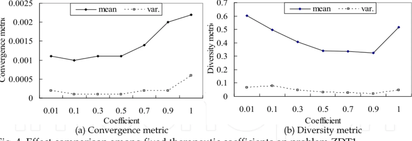
3) Effect of Therapeutic Coefficient
In the gene-therapy approach, each therapeutic gene of crossover child arithmetically combines two parity genes at the same locus of the mating parents. To test the effects of different therapeutic coefficient (coef), seven fixed coefficients and four variable ones for Equation (5) are tested on problem ZDT1. The mean and variance of the experimental results for seven fixed coefficients (from 0.01 to 1.0) are depicted in Fig. 4.The convergence metric depicted in Fig. 4(a) remains stable between 0.01 and 0.5. As the value of coef is larger than 0.5, the convergence situation is dramatically increased until coef=1. When the value of
coef increases from 0.01, the diversity metric in Fig. 4(b) is decreased and levels off between
0 0.01 0.02 0.03 0.04 0.05 10 20 30 40 50 60 70 80 90 100 Crossover percentage C on ve rg en ce m et ric mean var. 0 0.1 0.2 0.3 0.4 0.5 0.6 10 20 30 40 50 60 70 80 90 100 Crossover percentage D iv er sit y m et ric mean var.
(a)Convergence metric (b) Diversity metric
Fig. 2. Effect comparison among ten crossover percentages on problem ZDT1
d N d d d d d d l f N i i l f ) 1 ( 1 1
(10)The Euclidean distances between the extreme solutions of the Pareto front (P*) is df. The
distances between the boundary solutions of the obtained nondominated set (Q) is dl, and the distances between the consecutive solutions in the obtained non-dominated set is di. Notation d is the average of di.
3.2 Parameter Setting
To discover the best configuration for E-NSGA-II, some comprehensive investigations for parameter setting are performed on a benchmark problem. Especially, the performance of the evaluative crossover is influenced by three parameters: 1) crossover percentage; 2) crossover rate; and 3) therapeutic coefficient. The experimental results are averaged in 10 runs and evaluated by the convergence metric and the diversity metric. Problem ZDT1 is selected to analyze the effect of different parameters with a reasonable set of values in these experiments. The test function ZDT1 proposed by Zitzler et al. has a convex Pareto-optimal front and two objective functions without any constraint. The number of decision variables is 30 and the feasible region of each variable is in interval [0, 1].
( ), ( )
) ( Minimize T x f1 x1 f2 x (ZDT1) 1 1 1( ) where f x x (11)
1 / ( )
) ) ( ) ( 1 2 x g x x g x f (12) ) 1 /( ) ( 9 1 ) (x
2x n g in i . (13)1) Effect of Crossover Percentage
The crossover percentage decides how many successive individuals are produced by crossover operator. For example, 80% crossover percentage means that the crossover operator produces 80% offspring and the other 20% are produced by mutation operator. Especially, 100% crossover percentage means that all offspring are firstly recombined by crossover operator and then flipped one or more genes by mutation operator.
0 0.005 0.01 0.015 0.02 0.025 0.03 0.035 1 10 30 50 70 90 Crossover rate C on ve rg en ce m et ric mean var. 0 0.1 0.2 0.3 0.4 0.5 1 10 30 50 70 90 Crossover rate D iv er sit y m et ric mean var.
(a) Convergence metric (b) Diversity metric
Fig. 3. Effect comparison among ten crossover rates on problem ZDT1
To analyze the best percentage of crossover children in each generation, ten crossover percentages (from 10% to 100%) were tested on problem ZDT1. The mean and variance of the convergence and diversity metrics are depicted in Fig. 2(a) and Fig. 2(b), respectively. In Fig. 2(a), a larger crossover percentage implies a worse convergence situation when the crossover percentage is assigned from 10% to 90%. However, the best convergence is obtained when the crossover percentage is 100%. For diversity metric, Fig. 2(b) shows that the diversity metric is slightly declined from 10% to 70% and then rises until 90%. In particular, the best diversity metric is also obtained when the crossover percentage is 100%. Therefore, all individuals in this study are firstly recombined by the evaluative crossover and then mutated by the polynomial mutation.
2) Effect of Crossover Rate
In the gene-evaluation method, a smaller crossover rate implies a lower computational effort because only the selected loci in the therapeutic mask need to be evaluated individually. To realize the effects of different crossover rates (pc), six simulations with crossover rates from 1% to 90% are conducted on problem ZDT1 to discover the best crossover rate.
The convergence and diversity metrics of experimental results are depicted in Fig. 3(a) and 3(b), respectively. In Fig. 3(a), the convergence metric remains stable between pc=1% and
pc=10%. Obviously, a larger crossover rate implies a worse convergence situation on problem ZDT1 while pc is larger than 10%. The diversity metric in Fig. 3(b) is monotonically decreased from pc=1% to pc=10% and then slightly increased until pc=90%. Considering the convergence and diversity metrics, the crossover rate applied in this study is 10%.
3) Effect of Therapeutic Coefficient
In the gene-therapy approach, each therapeutic gene of crossover child arithmetically combines two parity genes at the same locus of the mating parents. To test the effects of different therapeutic coefficient (coef), seven fixed coefficients and four variable ones for Equation (5) are tested on problem ZDT1. The mean and variance of the experimental results for seven fixed coefficients (from 0.01 to 1.0) are depicted in Fig. 4.The convergence metric depicted in Fig. 4(a) remains stable between 0.01 and 0.5. As the value of coef is larger than 0.5, the convergence situation is dramatically increased until coef=1. When the value of
coef increases from 0.01, the diversity metric in Fig. 4(b) is decreased and levels off between
0 0.0005 0.001 0.0015 0.002 0.0025 0.01 0.1 0.3 0.5 0.7 0.9 1 Coefficient C on ve rg en ce m et ric mean var. 0 0.1 0.2 0.3 0.4 0.5 0.6 0.7 0.01 0.1 0.3 0.5 0.7 0.9 1 Coefficient D iv er sit y m et ric mean var.
(a)Convergence metric (b) Diversity metric
Fig. 4. Effect comparison among fixed therapeutic coefficients on problem ZDT1
0 0.0002 0.0004 0.0006 0.0008 0.001 0.0012 0.0014 0.0016 0.5~1 0~1 Increasing Decreasing Coefficient C on ve rg en ce m et ric mean var. 0 0.1 0.2 0.3 0.4 0.5 0.6 0.5~1 0~1 Increasing Decreasing Coefficient D iv er sit y m et ric mean var.
(a)Convergence metric (b) Diversity metric
Fig. 5. Effect comparison among variable therapeutic coefficients on problem ZDT1
E-NSGA-II Algorithm Setting
Population size 100
Maximum generation 1000
Simulation times 10
Percentage of offspring reproduction from crossover operator 100%
Percentage of offspring reproduction from mutation operator 100%
E-NSGA-II Crossover Operator
Crossover rate 0.1
Coefficient of arithmetical combination Random [0.5,1]
E-NSGA-II Mutation Operator
Mutation rate 1/ length of variable
Mutation scope Rank *20
Table 3. Parameter setting of E-NSGA-II
Fig. 5 depicts the experimental results of four variable type of therapeutic coefficients, which consist of 1) random value in interval [0.5, 1]; 2) random value in interval [0, 1]; 3) monotonically increasing value (from 0 to 1); and 4) monotonically decreasing value (from 1 to 0). Obviously, the random coefficient in interval [0.5, 1] achieves the best diversity metric in Fig. 5(b) although its convergence result in Fig. 5(a) is slightly worse than others about 0.0002. Considering the tradeoff between the convergence and diversity metrics, this study suggests the random value in interval [0.5, 1] as the therapeutic coefficient in this study.
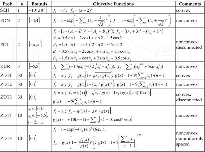
Table 4. Unconstrained test MOPs (All objectives are minimization functions) 3.3 Configuration of the E-NSGA-II
After these comprehensive experiments, the configuration and parameter setting of the proposed evaluative crossover are determined. Other parameters used in this study are the same as those in the original NSGA-II (Deb et al., 2002). The configuration of E-NSGA-II is summarized in Table 3 and used in the following section for performance comparison.
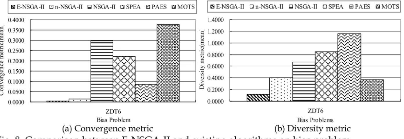
4. Computational Experiments
4.1 Test ProblemsNine test problems for MOPs are used in these experiments to systematically evaluate the performance of E-NSGA-II. These unconstrained benchmark problems suggested by Zitzler et al. cover a broad range of functionality characteristics with two objective functions (Zitzler et al., 2000). In this study, the test MOPs are denoted as SCH, FON, POL, KUR, ZDT1, ZDT2, ZDT3, ZDT4 and ZDT6. Table 4 describes the problem identifier, the number of variables, the feasible regions of decision variables, the function formulations, and the nature of the Pareto-optimal front for each problem (Deb et al., 2002).
Prob. n Bounds Objective Functions Comments
SCH 1
103,103
2; 1 x f 2 2(x2) f convex FON 2
4,4
31 2 1 3 1 2 1 ) 3 1 ( exp 1 ; ) 3 1 ( exp 1 i xi f i xi f nonconvex POL 2
,
2 2 1 1 2 2 2 1 1 1 2 1 2 2 2 1 2 2 2 2 2 1 1 1 cos 5 . 0 sin 2 cos sin 5 . 1 cos 5 . 1 sin cos 2 sin 5 . 0 2 cos 5 . 0 2 sin 2 1 cos 1 sin 5 . 1 2 cos 5 . 1 2 sin 1 cos 2 1 sin 5 . 0 ] ) 1 ( ) 3 [( ]; ) ( ) ( 1 [ x x x x B x x x x B A A x x f B A B A f nonconvex, disconnectedKUR 3
5,5 ( 10exp( 0.2 )); 1( 0.8 5sin 3))2 1 1 2 1 2 1
ni xi xi f in xi xi f nonconvex ZDT1 30
0,1 f1x1; f2g(x)
1 x1/g(x)
; g(x)19(
2x)/(n1) n i i convex ZDT2 30
0,1 ; ( )
1 ( / ( ))2
; ( ) 1 9( 2 )/( 1) 1 2 1 1x f g x x g x g x
x n f in i nonconvex ZDT3 30
0,1
) 1 /( ) ( 9 1 ) ( ) 10 sin( ) ( ) ( / 1 ) ( ; 2 1 1 1 2 1 1
x n x g x x g x x g x x g f x f n i i convex, disconnected ZDT4 10
n i x x i ,..., 2 , 5 , 5 1 , 0 1
n i xi xi n x g x g x x g f x f 2 2 1 2 1 1 ) 4 cos( 10 ) 1 ( 10 1 ) ( ) ( / 1 ) ( ; nonconvex ZDT6 10
0,1 1 2 2 0.25 2 1 6 1 1 1 9 1 ) ( ; ) ) ( ) ( ( 1 ) ( ); 6 ( sin ) 4 exp( 1
n x x g x g x f x g f x x f n i i nonconvex, nonuniformly spaced0 0.0005 0.001 0.0015 0.002 0.0025 0.01 0.1 0.3 0.5 0.7 0.9 1 Coefficient C on ve rg en ce m et ric mean var. 0 0.1 0.2 0.3 0.4 0.5 0.6 0.7 0.01 0.1 0.3 0.5 0.7 0.9 1 Coefficient D iv er sit y m et ric mean var.
(a)Convergence metric (b) Diversity metric
Fig. 4. Effect comparison among fixed therapeutic coefficients on problem ZDT1
0 0.0002 0.0004 0.0006 0.0008 0.001 0.0012 0.0014 0.0016 0.5~1 0~1 Increasing Decreasing Coefficient C on ve rg en ce m et ric mean var. 0 0.1 0.2 0.3 0.4 0.5 0.6 0.5~1 0~1 Increasing Decreasing Coefficient D iv er sit y m et ric mean var.
(a)Convergence metric (b) Diversity metric
Fig. 5. Effect comparison among variable therapeutic coefficients on problem ZDT1
E-NSGA-II Algorithm Setting
Population size 100
Maximum generation 1000
Simulation times 10
Percentage of offspring reproduction from crossover operator 100%
Percentage of offspring reproduction from mutation operator 100%
E-NSGA-II Crossover Operator
Crossover rate 0.1
Coefficient of arithmetical combination Random [0.5,1]
E-NSGA-II Mutation Operator
Mutation rate 1/ length of variable
Mutation scope Rank *20
Table 3. Parameter setting of E-NSGA-II
Fig. 5 depicts the experimental results of four variable type of therapeutic coefficients, which consist of 1) random value in interval [0.5, 1]; 2) random value in interval [0, 1]; 3) monotonically increasing value (from 0 to 1); and 4) monotonically decreasing value (from 1 to 0). Obviously, the random coefficient in interval [0.5, 1] achieves the best diversity metric in Fig. 5(b) although its convergence result in Fig. 5(a) is slightly worse than others about 0.0002. Considering the tradeoff between the convergence and diversity metrics, this study suggests the random value in interval [0.5, 1] as the therapeutic coefficient in this study.
Table 4. Unconstrained test MOPs (All objectives are minimization functions) 3.3 Configuration of the E-NSGA-II
After these comprehensive experiments, the configuration and parameter setting of the proposed evaluative crossover are determined. Other parameters used in this study are the same as those in the original NSGA-II (Deb et al., 2002). The configuration of E-NSGA-II is summarized in Table 3 and used in the following section for performance comparison.
4. Computational Experiments
4.1 Test ProblemsNine test problems for MOPs are used in these experiments to systematically evaluate the performance of E-NSGA-II. These unconstrained benchmark problems suggested by Zitzler et al. cover a broad range of functionality characteristics with two objective functions (Zitzler et al., 2000). In this study, the test MOPs are denoted as SCH, FON, POL, KUR, ZDT1, ZDT2, ZDT3, ZDT4 and ZDT6. Table 4 describes the problem identifier, the number of variables, the feasible regions of decision variables, the function formulations, and the nature of the Pareto-optimal front for each problem (Deb et al., 2002).
Prob. n Bounds Objective Functions Comments
SCH 1
103,103
2; 1 x f 2 2(x2) f convex FON 2
4,4
31 2 1 3 1 2 1 ) 3 1 ( exp 1 ; ) 3 1 ( exp 1 i xi f i xi f nonconvex POL 2
,
2 2 1 1 2 2 2 1 1 1 2 1 2 2 2 1 2 2 2 2 2 1 1 1 cos 5 . 0 sin 2 cos sin 5 . 1 cos 5 . 1 sin cos 2 sin 5 . 0 2 cos 5 . 0 2 sin 2 1 cos 1 sin 5 . 1 2 cos 5 . 1 2 sin 1 cos 2 1 sin 5 . 0 ] ) 1 ( ) 3 [( ]; ) ( ) ( 1 [ x x x x B x x x x B A A x x f B A B A f nonconvex, disconnectedKUR 3
5,5 ( 10exp( 0.2 )); 1( 0.8 5sin 3))2 1 1 2 1 2 1