How To Make A Query Safe On A Cloud Server

(1)

Fast Range Query Processing with

Strong Privacy Protection for Cloud Computing

Rui Li

1,3

_{Alex X. Liu}

2,3

_{Ann L. Wang}

2

_{Bezawada Bruhadeshwar}

3

College of Computer Science and Electronic Engineering, Hunan university, ChangSha, China1

Dept. of Computer Science and Engineering, Michigan State University, East Lansing, MI, U.S.A2

National Key Laboratory for Novel Software Technology, Nanjing University, Nanjing 210023, China3

Email: [email protected], [email protected], [email protected], [email protected]

ABSTRACT

Privacy has been the key road block to cloud computing as clouds may not be fully trusted. This paper concerns the problem of privacy preserving range query processing on clouds. Prior schemes are weak in privacy protection as they cannot achieve index indistinguishability, and therefore al-low the cloud to statistically estimate the values of data and queries using domain knowledge and history query results. In this paper, we propose the first range query process-ing scheme that achieves index indistprocess-inguishability under theindistinguishability against chosen keyword attack (IND-CKA). Our key idea is to organize indexing elements in a complete binary tree called PBtree, which satisfiesstructure indistinguishability (i.e., two sets of data items have the same PBtree structure if and only if the two sets have the same number of data items) and node indistinguishability (i.e., the values of PBtree nodes are completely random and have no statistical meaning). We prove that our scheme is secure under the widely adopted IND-CKA security model. We propose two algorithms, namely PBtree traversal width minimization and PBtree traversal depth minimization, to improve query processing efficiency. We prove that the worse case complexity of our query processing algorithm using PB-tree isO(|R|logn), wherenis the total number of data items andRis the set of data items in the query result. We imple-mented and evaluated our scheme on a real world data set with 5 million items. For example, for a query whose results contain ten data items, it takes only 0.17 milliseconds.

1. INTRODUCTION

1.1 Background and Motivation

Driven by lower cost, higher reliability, better perfor-mance, and faster deployment, data and computing services have been increasingly outsourced to clouds such as Ama-zon EC2 and S3 [1], Microsoft Azure [3], and Google App Engine [2]. However, privacy has been the key road block to cloud computing. On one hand, to leverage the computing and storage capability offered by clouds, we need to store

This work is licensed under the Creative Commons Attribution-NonCommercial-NoDerivs 3.0 Unported License. To view a copy of this li-cense, visit http://creativecommons.org/licenses/by-nc-nd/3.0/. Obtain per-mission prior to any use beyond those covered by the license. Contact copyright holder by emailing [email protected]. Articles from this volume were invited to present their results at the 40th International Conference on Very Large Data Bases, September 1st - 5th 2014, Hangzhou, China.

data on clouds. On the other hand, due to many reasons, we may not fully trust the clouds for data privacy. First, clouds may have corrupted employees who do not follow data privacy policies. For example, in 2010, a Google en-gineer broke into the Gmail and Google Voice accounts of several children [4]. Second, cloud computing systems may be vulnerable to external malicious attacks, and when in-trusions happen, cloud customers may not be fully informed about the potential implications on the privacy of their data. Third, clouds may base services on facilities in some foreign countries where privacy regulations are difficult to enforce.

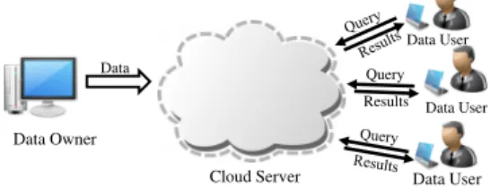
In this paper, we consider the following popular cloud computing paradigm: a data owner stores data on a cloud, and multiple data users query the data. For a simple exam-ple, a user stores his own data and queries his own data on the cloud. For another example, multiple doctors in a clinic store and query patient medical records in a cloud. Figure 1 shows the three parties in our model: a data owner, a cloud, and multiple data users. Among the three parties, the data owner and data users are trusted, but the cloud is not fully trusted. The problem addressed in this paper is range query processing on clouds in a privacy preserving and yet scalable manner. For a set of records where all records have the same attribute A, which has numerical values or can be represented as numerical values, given a range query specified by an interval [a, b], the query result is the set of records whose Aattribute falls into the interval. Range queries are fundamental operations for database SQL queries and big data analytics. In database SQL queries, thewhere

clauses often contain predicates specified as ranges. For ex-ample, SQl query select * from patients where 20 <=

age and age <= 30means to find all records of the patients

whose age is in the range of [20,30]. In big data analytics, many analyses involve range queries along dimensions such as time and human age.

Query Cloud Server Data Owner Data User Data User Data User Data Results

Figure 1: Cloud Computing Model

Given data items d1,· · ·, dn, the data owner encrypts these data using a symmetric key K, which is shared be-tween the data owner and data users, generates an in-dex, and then sends both the encrypted data denoted (d1)k,· · ·,(dn)kand the index to the cloud. Given a query,

(2)

the data user generates atrapdoor and then sends it to the cloud. The index and the trapdoor should allow the cloud to determine which data items satisfy the query. Yet, in this process, the cloud should not be able to inferuseful informa-tionabout the data and queries. The useful information in this context includes the values of the data items, the con-tent of the queries, and the statistical properties of the data items. Other than encrypted data and encrypted queries, to-gether with query results, the cloud may have information obtained from other channels, such as domain knowledge about the data (e.g., age distribution). However, even with such information, a privacy preserving range query scheme should not allow the cloud to infer additional information about the data based on past query results.

Besides privacy guarantees, a privacy preserving range query scheme should be efficient in terms of query process-ing time, storage overhead, and communication overhead. The query processing time needs to be small because many applications require real-time queries. The storage overhead refers to the data that cloud needs to store other than en-crypted data items. It needs to be small because the volume of data stored on the cloud is typically large. The commu-nication overhead refers to the data transferred between the data owner and the cloud, other than encrypted data items, and the data transferred between data users and the cloud, other than the precise query results. It needs to be small due to bandwidth limitations and the extra time involved in uploading and downloading.

1.2 Threat Model

For the cloud, we assume that the cloud is semi-honest (also called honest-but-curious), which was proposed by Canetti et al.in [13] and has been widely adopted includ-ing prior privacy preservinclud-ing range and keyword query work [8–11, 15–17, 19, 24–27, 31, 39]. A cloud is semi-honest means that it does follow required communication protocols and ex-ecute required algorithms correctly, but it may attempt to obtain information about the values of data items and the content of user queries with the help of domain knowledge about the data items and the queries (such as the distribu-tion of data items and queries). For the data owner and the data users, we assume that they are trusted.

1.3 Security Model

We adopt the IND-CKA security model proposed in [19], which has been widely accepted in prior privacy preserving keyword query work. This model has two key requirements: index indistinguishability (IND) andsecurity under chosen keyword attacks (CKA). Informally, a range query scheme is secure under the IND-CKA model if an adversaryAchooses two different sets S1 and S2 of data items, where the two sets have the same number of data items and they may or may not overlap, lets an oracle simulating the data owner to build indexes for S1 and S2, but A cannot distinguish which index is for which data set. The rationale is that if the problem is distinguishing the indexes for S1 and S2 is hard, then deducing at least one data item thatS1 and S2 do not have in common must also be hard. In other words, ifAcannot determine which data item is encoded in an in-dex with probability non-negligibly different from 1/2, then the index reveals nothing about the data items. Such in-dexes are calledsecure indexes. The IND-CKA model aims to prevent an adversaryAfrom deducing the plaintext val-ues of data items from the index, other than what it already

knows from previous query results or from other channels. Note that secure indexes do not hide information such as the number of data items. For applications that demand the privacy of data item numbers, they can inject dummy data items into small data sets to make all data sets to have equal sizes. Also, note that we are not interested in hiding search patterns, where a search pattern is defined as the set of trap-doors corresponding to different user queries. So far there are no searchable symmetric encryption schemes that can hide the statistical patterns of user searches because trapdoors are generated deterministically (i.e., the same trapdoor will always be generated for the same keyword) [27].

1.4 Summary and Limitation of Prior Art

Prior privacy preserving query schemes fall into two cat-egories according to their query types: range queries, which query all data items that fall into a given range, and keyword queries, which query all text documents that contain a given keyword. Privacy preserving range query schemes can also be called range searchable symmetric encryption schemes, and privacy preserving keyword query schemes can also be called keyword searchable symmetric encryption schemes. Prior privacy preserving range query schemes for the single-data-owner-multiple-data-user cloud paradigm fall into two categories: bucketing schemes [24–26] and order preserving schemes [9, 10, 31]. In bucketing schemes, the data owner partitions the whole data domain (e.g., [0,150] of human ages) into multiple buckets of varying sizes (e.g., 4 buckets of [0,12], [13,22], [23,60], [61,150]). The index consists of pairs of a bucket ID and the encrypted data items in the bucket. The trapdoor of a range query (e.g., [10,20]) consists of the IDs of the buckets that overlaps with the range (e.g., bucket IDs 1 and 2). All data items in a bucket are included in the query result as long as the bucket overlaps with the query. Bucketing schemes have two key limitations: weak privacy protection and high communication cost. Their privacy pro-tection is weak because the cloud can statistically estimate the actual value of both data items and queries using do-main knowledge and historical query results, as pointed out in [26]. Their communication cost is high because many data items in the query result do not satisfy the query. Reducing bucket sizes helps to reduce communication costs, but will worsen privacy protection because the number of buckets becomes closer to that of data items.

Order preserving schemes use encryption functions that preserve the relative ordering of data items even after en-cryption. For any two data items a and b, and an order preserving encryption function f, a ≤ b if and only if

f(a)≤f(b). In order preserving schemes, the index for data itemsd1,· · ·, dnaref(d1),· · ·, f(dn), and the trapdoor for query [a, b] is [f(a), f(b)]. Order preserving schemes have weak privacy protection because they allow the cloud to statistically estimate the actual values of both data items and queries [5].

The fundamental reason that the privacy protection pro-vided by the above prior schemes is weak is because their in-dexes are distinguishable for the same number of data items but with different distributions. In bucketing schemes, for the same number of data items, different distributions in data values will cause buckets to have different distributions in sizes because they need to balance the number of items among buckets. In order preserving schemes, for the same number of data items, different distributions in data values

(3)

will cause cipher-texts to have different distribution in the projected space. Leveraging domain knowledge about data distribution, both bucketing schemes and order preserving schemes allow the cloud to statistically estimate the values of data and queries.

1.5 Proposed Approach

In this paper, we propose the first privacy preserving range query scheme that achieves index indistinguishability. Our key idea for achieving index indistinguishability is to orga-nize all indexing elements in a complete binary tree where each node is represented using a Bloom filter, which we call aPBtree (where “P” stands for privacy and “B” stands for Bloom filter). PBtrees allow us to achieve index indistin-guishability because it has two important properties. First, a PBtree has the property ofstructure indistinguishability, that is, two sets of data items have the same PBtree struc-ture if and only if the two sets have the same number of data items. The structure of the PBtree of a set of data items is determined solely by the set cardinality, not the value of data items. Second, a PBtree has the property ofnode in-distinguishability, that is, for any two PBtrees constructed from data sets of the same cardinality, which have the same structure, and for any two corresponding nodes of the two PBtrees, the values of the two nodes are not distinguishable. Thus, our scheme prevents cloud from performing statistical analysis on the index even with domain knowledge.

1.6 Technical Challenges and Solutions

There are two key technical challenges. The first chal-lenge is the construction of PBtrees by data owners. We address this challenge by first transforming less-than and bigger-than comparisons into set membership testing (i.e., testing whether a number is in a set), which involves only equal-to comparisons, and then organize all the sets hierar-chically in a PBtree. This transformation helps us to achieve node indistinguishability because the less-than or bigger-than relationship among PBtree nodes is no longer statis-tically meaningful. The second challenge is the optimiza-tion of PBtrees for fast query processing on the cloud. We address this challenge by two ideas:PBtree traversal width minimizationandPBtree traversal depth minimization. The idea ofPBtree traversal width minimization is to minimize the number of paths that the cloud needs to traverse for pro-cessing a query. We prove that the PBtree traversal width minimization problem is NP-hard, and propose an efficient approximation algorithm. The idea ofPBtree traversal depth minimizationis to minimize the traversal depth of the paths that the cloud needs to traverse for processing a query; in other words, we want the traversal of many paths to termi-nate as early as possible.

1.7 Key Contributions

We make three key contributions. First, we propose the first privacy preserving range query scheme that is secure under the widely adopted IND-CKA model. Second, we pro-pose PBtrees, basic PBtree construction and query process-ing algorithms, and two PBtree optimization algorithms. Third, we implemented and evaluated our scheme on a large real world data set with 5 million data items. Experimental results show that our scheme is both fast and scalable. For example, for a query whose results contain ten data items, it takes only 0.17 milliseconds.

The rest of the paper proceeds as follows. We first review related work in Section 2. In Sections 3 and 4, we present our

basic PBtree construction and query processing algorithms and two PBtree optimization algorithms. In Section 5, we prove that our scheme is secure under the IND-CKA security model. In Section 6, we show our experimental results. We conclude the paper in Section 7.

2. RELATED WORK

There are some privacy preserving range query work that does not fit into our cloud computing paradigm and cannot be used to solve the problem addressed in this paper. In the public-key domain, the approach in [38] supports range querying using identity based encryption primitives [12, 37]. Their encryption scheme allows a network gateway to en-crypt summaries of network flows before submitting them to an untrusted repository; when a network operator suspects that an intrusion happens, a trusted third party can release a key to the operator to allow the operator to decrypt flows whose attributes fall within specified ranges, but not other flows. However, the user query privacy is not preserved.

A significant amount of work has been done in privacy preserving keyword queries [7,8,11,14–19,21,22,27,28,36,39]. However, these solutions are not optimized for range queries. Prior work on outsourced databases has addressed prob-lems such as secure kNN processing [32, 40, 41], privacy pre-serving data mining [6, 35], and query result integrity verifi-cation [30, 34, 42]. In [32, 40, 41], order preserving encryption techniques were used to compute the k-nearest neighbors of a given encrypted query point in an encrypted database. For the privacy preserving clustering mechanisms in [6, 35], certain confidential numerical attributes are perturbed in a uniform manner so that preserve the distances between any two points. Significant work has been done on query result integrity verification [30, 34, 42]. The basic idea is to include verifiable digital signatures for each returned tuple, which allow the client to verify the integrity of query results.

3. PBTREE CONSTRUCTION AND

TRAP-DOOR COMPUTATION

In this section, we first present our PBtree construction algorithm, which is executed by the data owner. This algo-rithm consists of three steps: prefix encoding, tree construc-tion, and node randomization using Bloom filters. Second, we present our algorithm for computing the trapdoor for a given query, which is executed by the data users. With the PBtree ofndata items and the trapdoor for a given query, the cloud is able to process the query on the PBtree without knowing the value of the data items and the query.

3.1 Prefix Encoding

The key idea of this step is to convert the testing of whether a data item falls into a range to the testing of whether two sets have common elements, where the basic step is testing whether two numbers are equal. To achieve this, we adopt the prefix membership verification scheme in [33]. Given a numberxof w bits whose binary representa-tion isb1b2· · ·bw, its prefix family denoted asF(x) is defined as the set of w+ 1 prefixes{b1b2· · ·bw, b1b2· · ·bw−1∗, · · ·,

b1∗· · · ∗,∗∗...∗}, where thei-th prefix isb1b2· · ·bw−i+1∗· · · ∗. For example, the prefix family of number 6 of 5 bits is

F(6) = F(00110) ={00110, 0011*, 001**, 00***, 0****, *****}. Given a range [a, b], we first convert the range [a, b] to a minimum set of prefixes, denoted S([a, b]), such that

(4)

the union of the prefixes is equal to [a, b]. For example,

S([0,8]) ={00***,1000}. Given a range [a, b], whereaandb

are two numbers ofwbits, the number of prefixes inS([a, b]) is at most 2w−2 [23]. For any numberxand range [a, b],

x∈ [a, b] if and only if there exists prefix p ∈ S([a, b]) so thatx∈pholds. Furthermore, for any numberxand prefix

p,x ∈p if and only if p∈ F(x). Thus, for any numberx

and range [a, b],x∈[a, b] if and only ifF(x)∩S([a, b])6=∅. From the above examples, we can see that 6 ∈ [0,8] and

F(6)∩S([0,8]) = {00∗ ∗∗}. In this step, given n data itemsd1,· · ·, dn, the data owner computes the prefix fam-ilies F(d1),· · ·, F(dn); given a range [a, b], the data user computesS([a, b]).

3.2 Tree Construction

To achieve sub-linear search efficiency, we organizeF(d1),

· · ·,F(dn) in a tree structure that we callPBtree. We cannot use existing database indexing structures likeB+ trees be-cause of two reasons. First, searching on such trees (such as B+ trees) requires the operation of testing which of two numbers is bigger; however, PBtrees cannot support such operations for the cloud because otherwise PBtrees will share the same weaknesses with prior order preserving schemes [24–26]. Second, their structures for different sets of data items are often different even if the two sets have equal sizes; however, for any two sets of the same size, their PBtrees are required to have the same structure,i.e., the two PBtrees are indistinguishable. In this paper, we orga-nizeF(d1),· · ·, F(dn) using our PBtree structure.

Definition 3.1 (PBtree). A PBTree forndata items

is a full binary tree withnterminal nodes andn−1 nonter-minal nodes, where alln terminal nodes form a linked list from left to right and each node is represented using a Bloom filter. Each terminal node contains one data item, and each nonterminal node contains the union of its left and right children. For any nonterminal node, the size of its left child either equals to that of its right child or exceeds by one.

According to this definition, a PBtree is a highly bal-anced binary search tree. The height of the PBtree for n

data items is ⌊logn⌋+ 1. We construct the PBtree from

F(d1),· · ·, F(dn) in a top-down fashion. First, we construct the root node, which is labeled with the n prefix families

{F(d1),· · ·, F(dn)}. Second, we partition the set ofnprefix families{F(d1),· · ·, F(dn)}into two subsets of prefix fam-iliesSleft and Sright such that|Sleft|=|Sright|ifnis even

and|Sleft|=|Sright|+ 1 ifnis odd, and then construct two

child nodes for the root, where the left child is labeled with

Sleft and the right child is labeled with Sright. We

recur-sively apply the above step to the left child and the right child, respectively, until every terminal node contains only one prefix family. At the end, we link all terminal nodes by a linked list. Figure 2 shows the PBtree for the set of prefix familiesS={F(1),F(6),F(7),F(9),F(11),F(12),F(13),

F(16),F(20),F(25)}.

The key property of PBtrees is stated in Theorem 3.1, which is straightforward to prove according to its construc-tion algorithm. Note that the constraint 0 ≤ |Sleft| −

|Sright| ≤ 1 makes the structure of the PBtree for a set

of data items to solely depend on the number of data items.

Theorem 3.1 (Structure Indistinguishability).

For any two sets of data items S1 and S2, their PBtrees have exactly the same structure if and only if|S1|=|S2|.

F(1), F(6), F(7), F(9) ,F(11), F(12), F(13), F(16), F(20), F(25) F(1), F(6), F(7),F(16), F(20) F(9), F(11), F(12),F(13), F(25) F(1), F(6), F(7) F(16), F(20) F(12), F(13), F(25) F(6),F(7) F(1) F(6) F(7) F(20) F(16) F(12), F(13) F(12) F(13) F(25) F(9) F(11) F(9), F(11)

Figure 2: PBtree Example

We now describe the query processing algorithm on the above tree. For a PBtreeT, we useT.rootto denote the root node ofT,T.lef tto denote the left subtree ofT, andT.right

to denote the right subtree ofT. For a nodev, we useL(v) to denote the label of v, which is a set of prefix families, andU(v) to denote the union of all prefix families inL(v). For example, if L(v) ={F(6), F(7)}, then U(v) = F(6)∪ F(7). Given a range [a, b], starting from the root T.root

of a PBtree T, where L(T.root) = {F(d1),· · ·, F(dn)}

and U(T.root) = F(d1)∪ · · · ∪F(dn), we check whether

U(T.root)∩S([a, b]) =∅. IfU(T.root)∩S([a, b]) =∅, then

none of then data itemsd1,· · ·, dn falls into the range of [a, b] and therefore we do not need to continue searching tree

T. IfU(T.root)∩S([a, b])6=∅, then there exists at least one

of then data itemsd1,· · ·, dn falls into the range of [a, b]; thus, we need to continue to recursively conduct the same search onT.lef tandT.right, if they exist. The pseudocode of the algorithm is in Algorithm 1.

Algorithm 1: PBtreeSearch(T, a, b) Input:S

Output: PBtree nodes whose data item is in [a, b]

1 if U(T.root)∩S([a, b]) =∅then 2 returnnull ; 3 else 4 if T is leaf then 5 returnL(T.root); 6 else 7 PBtreeSearch(T.lef t, [a, b]); PBtreeSearch(T.right, [a, b]);

Now, we analyze the time complexity of our query process-ing algorithm 1 and show that it is sub-linear in the number of data items. Letnbe the number of data items indexed by the PBtree, [a, b] be the query, and R be the query result. The average run-time of the search algorithm depends on

|R|, the number of data items in the query result. Theoreti-cally, if|R|= 0, then only the root of the PBtree needs to be checked and the time complexity isO(1); if|R|=n, then all data items indexed by the PBtree need to be traversed via the linked list and the time complexity isO(n). In reality, we have|R| ≪nasnis typically large. For each data item in R, we need to traverse at most 2 logn−1 nodes. Thus, the time complexity isO(|R|logn)

3.3 Node Randomization Using Bloom Filters

Next, we present a solution based on secure keyed hash functions (HMAC) and Bloom filters to make our PBtree privacy preserving. For each node v, we use a Bloom filter denoted byv.B to store the prefixes of a node’s prefix fam-ilies. We assume that the data owner and the users share

(5)

rsecret keys, denotedk1,· · ·, kr, other than the symmetric key for encrypting and decrypting data items. Consider a PBtree nodev, where set L(v) consists ofnprefix families and setU(v) consists ofmprefixesp1,· · ·, pm. Letwbe the number of bits that each data item contains. Our node ran-domization algorithm consists of the following three steps.

One-wayness: For each prefixpi, we use thersecret keys to compterhashes:HMAC(k1, pi),· · ·,HMAC(kr, pi). The pur-pose of this step is to achieve one-wayness, that is, given prefix pi and the r secret keys, it is computationally effi-cient to compute ther hashes; but given therhashes, it is computationally infeasible to compute thersecret keys and

pi; furthermore, even given therhashes andpi, which is the case in chosen plaintext attacks (CPA), it is still computa-tionally infeasible to compute thersecret keys.

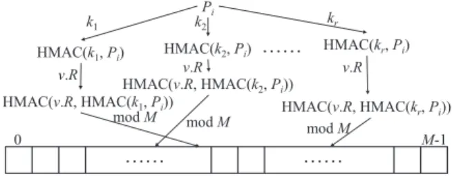
Decorrelation: For node v, we generate a random num-berv.R, which has the same number of bits as a secret key. We use v.R to compute r hashes: HMAC(v.R,HMAC(k1, pi)),

· · ·,HMAC(v.R,HMAC(kr, pi)). For each prefixpi and for each 1≤j≤r, we let v.B[HMAC(v.R,HMAC(kj, pi))mod M] := 1. The purpose of the random number that is unique for each node is to eliminate the correlation among different Bloom filters for different nodes. For the same prefix p, this ran-dom number allows us to hashpindependently for different Bloom filters. Without the use of this random number, if prefixpiis shared byU(v1) andU(v2) of two different nodes

v1 andv2, then for all therlocationsHMAC(k1, pi) mod M,

· · ·,HMAC(kr, pi)mod M, both Bloom filters have the value 1. Although two Bloom filters both having 1 for all theser

locations does not necessarily mean that U(v1) and U(v2) share a common prefix, without the use of this random num-ber, if two Bloom filters have more 1s at the same locations than other pairs, then the probability that they share com-mon prefixes is higher. Figure 3 shows the above hashing process for Bloom filters.

Pi HMAC(k1, Pi) k₁ HMAC(k2, Pi) …… HMAC(kr, Pi) k₂ kr HMAC(v.R, HMAC(k₁, P_i)) HMAC(v.R, HMAC(k2, Pi)) HMAC(v.R, HMAC(kr, Pi)) v.R v.R v.R …… …… 0 M-1 mod M _mod_M mod M

Figure 3: Secure Hashing in Bloom filters

Padding: Ifm <(w+1)∗n, which means that some prefix families share common prefixes, we generate ((w+1)∗n−m)∗ rrandom numbers and for each numberx,v.B[x mod M] := 1. At last, we use this Bloom filter together with the random numberv.R to replace the label of v. The purpose of this step is to avoid a Bloom filter to expose the information how much its prefix families share common prefixes. Without the padding, some Bloom filters are inserted with less number of elements than others, which will cause it to have less 1s than others in the statistical sense.

By now the PBtree is fully constructed from data items

d1,· · ·, dn by the data owner. The data owner sends the encrypted data items and the PBtree to the cloud.

3.4 Trapdoor Computation

Given a query [a, b], suppose S([a, b]) consists of z pre-fixesp1,· · ·, pz, for each prefixpi, 1≤i≤z, the data user

d_j-₁ d_j d_j+₁ d_j+₂ d_l

…

Figure 4: PBtree Example

computesrhashes:HMAC(k1, pi),· · ·,HMAC(kr, pi). The trap-door for query [a, b], denoted asM[a,b], is a matrix of z∗r hashes:HMAC(k1, p1),· · ·,HMAC(kr, p1),· · ·,HMAC(k1, pz),· · ·,

HMAC(kr, pz). We organize thesez∗rhashes in a matrix be-cause the cloud needs to know whichrhashes are all corre-spond to the same prefix. The trapdoor ofpicorresponds to theith row of the trapdoor matrix. After the computation, the data user sendsM[a,b]to the cloud.

3.5 Query Processing

After receiving a query represented as a trapdoor, the cloud uses the trapdoor to search over the PBtree. The query processing algorithm on PBtrees (i.e., Algorithm 1) still ap-plies except that the checking of whetherU(v)∩S([a, b])6=∅

is implemented as checking whether there exists a row

i(1≤i≤z) in matrixM[a,b]so that for everyj(1≤j≤r) we havev.B[HMAC(v.R,HMAC(kj, pi))mod M] = 1.

The straightforward implementation of the above query processing algorithms requires to check each row ofM[a,b]at each visited PBTree node. Note that for a rowiinM[a,b], if there existsj(1≤j≤r) so thatv.B[HMAC(v.R,HMAC(kj, pi))

mod M] = 0, thenU(v)∩pi=∅. IfU(v)∩pi=∅, then for any

descendent nodev′_{of node}_v_{, we have}_U₍_v′₎_∩_p

i=∅because

U(v′₎ _⊂_U₍_v_{). Based on this fact, when we take}_M [a,b] to search over the PBtree, for any such row inM[a,b], we remove it from M[a,b] when we continue to search the descendent nodes of v. The searching process terminates when M[a,b] becomes empty or we finish searching terminal nodes.

3.6 False Positive Analysis

As each node in a PBtree is represented by a Bloom filter, which inherently has false positives, the query result on a PBtree may contain false positives. For simplicity, consider a PBtree with n = 2hleaf nodes, where the height of the PBtree ish+ 1. LetRbe the query result, which is a set of data items. We color all the terminal and nonterminal nodes on the path from a data item inRto the root of the PBtree to be grey and others to be white. Figure 4 shows such a marked PBtree where dj ∈ R. Let f be the false positive rate of a Bloom filter in the PBtree. Note that although nodes of different levels in a PBtree may have a Bloom filter of different length, we always choose the number of hash functionsrto be m

n×ln 2 to minimize the false positive rate to be (1−(1− 1

m rn

)r_≈₍₁₋_e−rn/m₎r_{= 2}−r_≈₀_.₆₁₈₅m/n_; thus, by choosing the same m/n value for each node, the false positive of the Bloom filter at each node is the same. For any nodedi∈/R, letlen(di, R) be the number of white nodes on the path fromdito the root, the probability thatdi is a false positive isflen(di,R)_{. Thus, the expected number of}

false positives is Σdi∈/Rf

len(di,R)_{. Among all possible query}

result setsR of the same size a, we useMa be denote the maximum expected number of false positives. Thus,

Ma= max ∀R (

X

di∈/R

(6)

Fora= 0, we have

M0= 2h×ph+1 (3.2) Fora= 1, saydj∈Ras illustrated by Figure 4, the values of len(di, R) for di ∈/ R are 1,2,2,3,3,3,3,· · ·. Thus, we have:

M1=f+ 2f2+· · ·+ 2h−1fh=f1−(2f) h

1−2f (3.3)

For 1 < a ≤ n, according to Equation 3.1, Ma corre-sponds to the case where in the (⌈loga⌉+ 1)-th layer there are a nodes colored grey and for each subtree rooted at thesea nodes, there is one and only one terminal node is colored grey. Considering the 2⌈loga⌉subtrees rooted at the (⌈loga⌉+ 1)-th layer, theasubtrees have only one grey ter-minal node each and the rest 2⌈loga⌉−asubtrees have no grey terminal nodes. For each of theasubtrees, we can calcu-late the maximum expected number of false positives based on Equation 3.3; similarly, for each of the rest 2⌈loga⌉−a

subtrees, we can calculate that based on Equation 3.2. Thus,

Macan be calculated as follows:

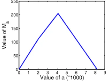
Ma=af×

1−(2f)h−⌈loga⌉ 1−2f + (2

⌈loga⌉

−a)f(2f)h−⌈loga⌉ Figure 5 shows the relation betweenMaanda, where we choosef= 0.05 andh= 13. 0 1 2 3 4 5 6 7 8 9 0 50 100 150 200 250 Value of a (*1000) Value of M a

Figure 5: Relation betweenMa and a

4. PBTREE SEARCH OPTIMIZATION

In this section, we optimize PBtree searching efficiency by minimizing the number of nodes that a query needs to traverse both horizontally and vertically.

4.1 Traversal Width Optimization

Recall that in the PBtree construction algorithm in Sec-tion 3.2, for a nonterminal node with prefix family setS, we partition this node into two child nodes S1, S2 so that 0≤ |S1| − |S2| ≤1. This partition is critical for the perfor-mance of query processing on the PBtree because querying the common prefixes that bothS1 andS2share will lead to the traversal of both subtrees. Thus, in partitioningS into

S1, S2, besides satisfying the condition 0≤ |S1| − |S2| ≤1, we want to minimizeM ax{Fi∩Fj|Fi∈S1, Fj∈S2}, which is the maximum number of prefixes in the intersection of two prefix families that one fromS1and the other fromS2. This condition is to let those prefix families that share more pre-fixes to be partitioned in the same set. We call this problem Equal Size Prefix Family Partition. We next formally define this problem and prove that it is NP-hard.

Definition 4.1 (Equal Size Prefix Family Partition).

Given a setSof prefix families, we want to partitionS into

S1, S2, such that the following two conditions are satisfied:

1. 0≤ ||S1| − |S2|| ≤1;

2. M ax{Fi∩Fj|Fi∈S1, Fj∈S2}is minimized.

Theorem 4.1. The Equal Size Prefix Family Partition

problem is NP-hard.

Proof. The decision version of the Equal Size Prefix

Family Partition Problem is the following: “Is it possible to partition a set S of prefix families into S1 and S2 such that 0≤ ||S1| − |S2|| ≤1 and M ax{Fi∩Fj|Fi ∈S1, Fj ∈

S2}< k?” We reduce theSet Partition Problem, a known

NP-Complete problem, to the decision version of Equal Size Prefix Family Partition Problem. The Set Partition Problem is as follows: “For a multiset of positive numbers

A = {a1, a2,· · ·, an}, is it possible to partitionA into A1 andA2 such thatP_a_i_∈_A1ai=

P

aj∈A2aj”.

Given an instance of the set partition problem with pos-itive number multiset A = {a1, a2,· · ·, an}, we convert it to an instance of our Equal Size Prefix Family Partition Problem with prefix family set S as follows. Let amax be the largest number inA. For each numberai inA, we first generateaidata itemsd1, d2,· · ·, dai where each data item

has ⌈logn⌉+⌈logamax⌉ bits, and for each data item dj (1 ≤ j ≤ ai), the value of the first ⌈logn⌉ bits is i and the value of the last ⌈logamax⌉bits is j−1. For example, suppose A = {2,3,4}, for number 2 in A, we generate 2 data items 0000 and 0001 in their binary representation. Second, for each data itemdj (1≤j≤ai), we generate its prefix family F(dj). Finally, we map each number ai in A to ai prefix families F(d1), F(d2),· · ·, F(dai) in S, and let k=⌈logn⌉.

Suppose the prefix family set S constructed above has an equal size prefix family partition solution S1 and S2 with M ax{Fi∩Fj|Fi ∈ S1, Fj ∈ S2} ≤ k = ⌈logn⌉. We next prove thatAhas a set partition solution. Note that if

P

ai∈Aaiis odd, then the set partition problem has no

solu-tion. Thus, we only need to consider cases where P_a

i∈Aai

is even, which means that|S1|=|S2|. A notable property of the ai prefix families F(d1), F(d2),· · ·, F(dai) constructed

above is that any two of these prefix families share at least

⌈logn⌉prefixes. For example,F(0001) andF(0001) share 3 prefixes. Thus,M ax{Fi∩Fj|Fi∈S1, Fj∈S2} ≤k=⌈logn⌉ implies that for anyai inA, the constructedai prefix fam-ilies F(d1), F(d2),· · ·, F(dai) are either all in S1 or all in S2. Otherwise, suppose F(d1) ∈ S1 and F(d2) ∈ S2, then

|F(d1)∩F(d2)| ≥ ⌈logn⌉ = k. Thus, |S1| is equal to the sum of some numbers in A and |S1| is equal to the sum of the remaining numbers inA. Finally,|S1|=|S2|implies thatAhas a set partition solution. Thus, the Set Partition Problem≤pthe decision version of Equal Size Prefix Family Partition Problem, which means that the Equal Size Prefix Family Partition Problem is NP-hard.

Next, we present our approximation algorithm to the equal size prefix family partition problem. Our algorithm consists of two phases: partition phase and re-organization phase. In the partition phase, we partition the input prefix family set into two or three subsets so that the size of each subset is no larger than⌈n

2⌉, wherenis the size of the pre-fix family set. In the re-organization phase, if the first phase outputs two subsets, then we do nothing because the two subsets must satisfy the condition of 0≤ ||S1| − |S2|| ≤1; if the first phase outputs three subsets, then we first choose one subset to split into multiple smaller subsets, and then merge

(7)

these new subsets with the two other subsets to obtain two subsets that satisfy the condition of 0≤ ||S1| − |S2|| ≤1.

To help to present the details of these two phases, we first define two concepts: longest common prefix and child prefixes. The longest common prefix of a set of prefix families

S = {F1, F2,· · ·, Fn}, denoted by LCP(S), is the longest prefix inF1∩F2∩· · ·∩Fn. For example, the longest common prefix of{F(1101), F(1100)}is 110∗. Note that for any set of prefix families, it has only one longest common prefix because no prefix family consists of two prefixes of the same length. For any prefixb1b2· · ·bw−i+1∗ · · · ∗, it has two child prefixes b1b2· · ·bw−i+10∗ · · · ∗ and b1b2· · ·bw−i+11∗ · · · ∗, which are obtained by replacing the first∗by 0 and 1 and called child-0 and child-1 prefixes, respectively. For example, prefix 11∗ ∗has two child prefixes 110∗ and 111∗. For any prefixp, we usep0 _and _p1 _{to denote}_p_{’s child-0 and child-1} prefixes, respectively.

Given a set of prefix families S = {F1, F2,· · ·, Fn}, the partition phase of our approximation algorithm works as follows. First, we compute LCP(S), the longest common prefix of S. Second, we partition S into two subsets, one subset whose each prefix family containsLCP(S)0 _{and one} subset whose each prefix family containsLCP(S)1. If any of the two subsets has a larger size than⌈n

2⌉, then we recur-sively apply the above two partition process to that subset. This process terminates when all subsets have a smaller size than ⌈n

2⌉. Third, for any two subsets whose union has a size smaller than⌈n

2⌉, we call themmergeableand we merge them (i.e., union them into one set). This process terminates when no two subsets are mergeable. Thus, we result in ei-ther two subsets or three subsets. It is impossible to result in four subsets or more because otherwise there are at least two subsets can be merged.

If the partition phase results in two subsets, then the re-organization phase does nothing. LetS1 andS2 be the two subsets. Because|S1|+|S2|=n,|S1| ≤ ⌈n₂⌉, and|S2| ≤ ⌈n₂⌉, we have 0≤ ||S1| − |S2|| ≤1. Thus,S1 andS2 represent the final partition result.

If the partition phase results in three subsets, then the re-organization phase chooses one subset to split into multi-ple smaller subsets, and then union these new subsets with the two other subsets to obtain two subsetsS1 andS2 that satisfy the condition of 0≤ ||S1| − |S2|| ≤1. LetS1,S2, and

S3be the three subsets. We choose the subset whose longest common prefix is the smallest, that is, the subset whose prefix families share the least number of prefixes. Let S3 be the subset that we choose. We first compute its longest common prefix LCP(S3). Note that for any prefix family in S3, it contains either LCP(S3)0 or LCP(S3)1. Second, we split S3 into two subsets S31, whose each prefix fam-ily contains LCP(S3)0_{, and}_S_{32, whose each prefix family} containsLCP(S3)1. Without loss of generality, we suppose

|S31| ≤ |S32|. Thus, eitherS1orS2can be merged withS31. Otherwise, if both|S1|+|S31|>⌈n₂⌉and|S2|+|S31|>⌈n₂⌉, then|S1|+|S2|+|S3|=|S1|+|S2|+|S31|+|S32| ≥ |S1|+|S2|+

|S31|+|S31|= (|S1|+|S31|) + (|S2|+|S31|)>⌈n₂⌉+⌈n₂⌉ ≥n. Again, suppose|S1| ≥ |S2|andS1 can be merged withS31, we mergeS1withS31. After mergingS1withS31, we check whetherS2 can be merged withS32. If they can, we merge them and output the partition resultS1∪S31andS2∪S32. IfS2 and S32 can not be merged, we further splitS32, and repeat the above process. IfS1 can not be merged withS31, we merge S31 with S2 and split S32, and then repeat the

above process. The pseudocode of this algorithm is shown in Algorithm 2.

We now analyze the worst case computational complexity of Algorithm 2. Let n be the size of the input set of pre-fix families and T(n) be the corresponding time complex-ity. Each set partition operation takes O(n) time and each subset merging takesO(1) time. The worse case time com-plexity is when each set partition operation produces two subsets where the size of one subset is one. Thus, we have:

T(n) =T(n−1) +O(n). The computational complexity of Algorithm 2 is thereforeO(n2_{) in the worst case.}

Algorithm 2: EqualSizePrefixFamilyPartition(S) Input:S={F1, F2,· · ·, Fn}

Output:S1 andS2whereS1⊂S,S2⊂S, and 0≤ ||S1| − |S2|| ≤1

1 Initiate an empty partition subset listL. 2 while(|S|>⌈n

2⌉)do

3 ComputepSfor S. ParitionS into

S1={∀Fi|LCP(S)0∈Fi, Fi∈S}, and S2={∀Fi|LCP(S)1∈Fi, Fi∈S}. 4 if (|S1| ≥ |S2|)then 5 InserteS2intoL;S:=S1. 6 else 7 InsertS1 intoL;S:=S2. 8 InsertS intoL.

9 while(subsetsSi andSj are mergable inL)do 10 MergeSi andSjinto one subsetSij. ReplaceSi

andSj withSijinL.

11 if Lcontains only two subsetsS1 andS2 then 12 returnS1 andS2.

13 else

14 LetS3 be the subset that has| ∩Fi∈S3| ≤ | ∩Fi∈S1|, and| ∩Fi∈S3| ≤ | ∩Fi∈S2|holds.

15 whileLhas 3 subsets denoted byS1,S2, andS3 do 16 RemoveS3 fromL. SplitS3intoS31, andS32.

Let|S1| ≥ |S2|, and|S31| ≤ |S32|. 17 if (|S1|+|S31| ≤ ⌈n₂⌉)then 18 MergeS31withS1. 19 if (|S2|+|S32| ≤ ⌈n₂⌉)then 20 MergeS32 withS2. 21 else 22 S3 :=S32. InsertS3intoL. 23 else 24 MergeS31withS2. 25 S3:=S32. InsertS3 intoL. 26 returnLabels of the two subsets inL.

4.2 Traversal Depth Optimization

Our idea for optimizing searching depth is based on the following observation: for any internal node v with label

{F(d1), F(d2),· · ·, F(dm)} that a query prefixptraverses, ifp∈F(d1)∩F(d2)∩ · · · ∩F(dm), then all terminal nodes of the subtree rooted at v satisfy the query; thus, we can directly jump to the left most terminal node of this subtree and collect all terminal nodes using the linked list, skipping

(8)

the traversal of all nonterminal node underv in this sub-tree. This optimization opportunity is the motivation that we chain the terminal nodes in PBtrees. Note that here

F(d1)∩F(d2)∩ · · · ∩F(dm) 6= ∅because it must contain the prefix of w *s. Furthermore, our searching width op-timization technique significantly increases the probability that the prefix families in a nonterminal node share more than one common prefix.

For a node v labeled with {F(d1), F(d2),· · ·, F(dm)}, we split Sm_i=1F(di) into two sets: the common set C ₌

Tm

i=1F(di) and the uncommon set N =

Sm

i=1F(di) −

Tm

i=1F(di). With this splitting, query processing at node

v is modified to be the following. First, we check whether

p∈N_{. If}_p_∈N_{, then we continue to use the query processing} algorithm in 3.5 to searchponv’s left and right child nodes. Ifp /∈N, then we further check p∈C; ifp /∈Nbutp∈C, then we directly jump to the bottom to collect all terminal nodes in the subtree rooted atv; if pis in neither set, then we skip the subtree rooted atv.

The key technical challenge in searching depth optimiza-tion is how to store the common setCand the uncommon set N for each nonterminal node using Bloom filters. The straightforward solution is to use two Bloom filters, stor-ing Cand N, respectively. However, this will not be space efficient as we need two bit vectors. In this paper, we pro-pose an space efficient way to represent two Bloom filters using two sets ofk hash functions {hc1, hc2,· · ·, hcr} and

{hn1, hn2,· · ·, hnr} but only one bit vector B of m bits. In the PBtree construction phase, for a prefixp ∈ C_∪N_, ifp∈C_{, we set}_B_[_hc₁₍_p_)]_{, B}_[_hc₂₍_p_)]_,_{· · ·}_{, B}_[_hc_r(_p_{)] to be 1;} ifp ∈ N, we setB[hn1(p)], B[hn2(p)],· · ·, B[hnr(p)] to be 1. Thus, we check whether a p ∈ C by checking whether

∧r

i=1(B[hci(p)] == 1) holds and check whether p ∈ N by checking whether∧r

i=1(B[hni(p)] == 1) holds.

Next, we analyze the false positives of this Bloom filter with two sets ofr hash functions and a bit vectorB ofm

bits. Suppose we have insertednelements (i.e.,|C_|₊_|N_|₌

n) into this bloom filter. Recall that our query processing algorithm conducts two times of set membership testing of a query prefix p at node v: first, we test whether p ∈ N; second, on the condition thatp /∈ N, we test whether p∈

C_{. Let} _fN be the probability of a false positive occurs at

the first membership testing, andfC be the probability of

a false positive occurs at the second membership testing. As thenelements are randomly and independently inserted into the bit vectorB, the false positive probability at the first membership testing is the same as the false positive probability of the standard Bloom filter. Thus, we have

fN= (1−(1−

1

m)

rn

)r= (1−e−rnm₎r _(4.1)

As the second testing is only performed on the condition thatp /∈N, and similarly, when the conditionp /∈Nholds, the false positive probability at testing whetherp∈Cis the same as that at testing whetherp∈N_{, we have}

fC= (1−fN)×(1−(1− 1 m) rn₎r_{= (1} −(1−e−rnm)r)×(1−e− rn m)r (4.2) To further reduce the false positive probability in testing

p∈C_{at node} _v_{, when we collect the leaves of the subtree} rooted at v, we can randomly choose xleaf nodes to test whether they indeed matchp; if any of the leaf nodes does not match p, which means that p /∈ C, then we exclude all leaves of the subtree rooted atv from the query result.

Thus, with the testing of thexleaf nodes, the false positive probability in testing whetherp∈Cbecomes the following:

fC×(1−e−

rn

m)rx= (1−(1−e−rnm)r)×(1−e−rnm)rx+r (4.3)

Note that we testp∈N_{first and only when}_{p /}_∈N_{we test}

p∈C_{. Otherwise, if we use the above mentioned leaf testing} method to further reduce the false positive probability in testing p ∈ C_{, we may introduce false negatives, which is} not allowed in our scheme. Suppose we first testp∈C_first and only when p /∈ C we test p ∈ N. For a query prefix

p, if p ∈N _and_{p /}_∈C_{, but false positive occurs in testing}

p /∈C_{, when we collect the leaves of the subtree rooted at}

v, if we test a leaf node and find it is not in C, according to the above leaf testing method, we exclude all leaves of the subtree rooted at v from the query result; however, as

p∈N, some of these excluded leaves should be included in the query result, which are false negatives.

5. SECURITY ANALYSIS

5.1 Security Model

To achieve IND-CKA security, our PBtree uses pseudo-random functions, which are keyed functions and cannot be distinguished from a truly random function with non-negligible probability [29]. Letg:{0,1}n_×{₀_,₁_}s_{→ {}₀_,₁_}m be a keyed function which takes as inputn-bit strings and

s-bit keys and maps to m-bit strings. Let G : {0,1}n _→

{0,1}m_{be a random function which maps}_n_{-bit strings to}_m -bit strings. Now,gis a pseudo-random function if, for a fixed value k ∈ {0,1}s_{, the function} _g₍_{x, k}_{), where} _x _{∈ {}₀_,₁_}n_, can be computed efficiently and if a probabilistic polyno-mial time adversaryAwith access to r chosen evaluations of g, i.e., (xi, g(xi, k)) where i∈ [1, r], cannot distinguish the valueg(xr+1, k) from the output of a random function

G with non-negligible probability. We have used HMAC for our scheme as the pseudo-random function. From the re-sults in [17, 29], a searchable symmetric encryption scheme is secure if a probabilistic polynomial time adversary cannot distinguish between the output of a real index, which uses pseudo-random functions, and a simulated index, which uses random functions, with non-negligible probability. We show the construction of such a simulator for our scheme and thereby, prove its security under the IND-CKA model.

5.2 Security Proof

Without loss of generality, we view the PBtree as a list of Bloom filters, where each Bloom filter stores a distinct set of prefixes and answers user queries. Therefore, we note that, that the proof of security of PBtree is equivalent to proving that any given Bloom filter is IND-CKA secure satisfying the following properties: (a) the contents of the data items are not revealed from the structure of the Bloom filter in which they are stored or from the contents of other Bloom filters, and (b) given any two Bloom filters, with different number of data items, they are indistinguishable to an ad-versary. We consider a non-adaptive adversary, which has a one-time finite trace of the search history consisting of a finite set of secure trapdoors and their corresponding search results. To complete the proof, we demonstrate the construc-tion of a probabilistic polynomial time simulator S, which can simulate the secure index using only this finite trace of the search history. The adversary interacts with the simula-tor as well as the real index and is challenged to distinguish between the results of the two indexes with non-negligible

(9)

probability. We consider the length of the keysas the secu-rity parameter in the following definitions:

History:Hq. LetD={D1, D2,· · ·, Dn}denote the set of data items whereDidenotes theith data item. LetR1:q= {R1, R2,· · ·, Rq}, denote a sequence of q range queries where each range query is of the form, Ri = {ai, bi} for

ai, bi, q∈N. The history Hq is defined asHq ={D,R1:q}, where the set D consists of data items, which match one or more of the range queries inR1:q. An important

require-ment is thatqmust be polynomial in the security parameter

s, the key size, in order for the adversary to be polynomially bounded.

Adversary View: Av. This is the view of the adversary of a history Hq. Each range query, Ri = {ai, bi} gener-ates a set of ri trapdoors, Ti = {ti,1, ti,2,· · ·, ti,ri} which

are secure under an encryption keyK. Now, the adversary view consists of: the set of trapdoors corresponding to the range queriesT, the secure index I for D and, set of the encrypted data items,EncK(D)={EncK(D1), EncK(D2),

· · ·,EncK(Dn)}. Formally,Av(Hq) ={T;I;EncK(D)}. In addition, the adversary may also know the size of the en-crypted data items.

Result Trace This is defined as theaccessandsearch pat-terns observed by the adversary afterTis matched against the encrypted index I. The access pattern is the set of matching data items, M(T)={ m(t1), m(t2) · · ·, m(tq)}, where m(ti) denotes the set of matching data item iden-tifiers for trapdoor ti. The search pattern is a symmetric binary matrixΠT defined overT, such that,ΠT[p, q] = 1 if

tp=tq, for, 1≤p, q≤σ|Ti|. We denote the matching result trace overHq as:M(Hq)={M(R1:q), ΠT[p, q]}. The

adver-sary can only see a set of matching data items for each trap-door, which is captured using these two patterns. Therefore, each Bloom filter can be viewed as a match for a distinct, but not necessarily unique when viewed along the PBtree, set of trapdoors. The uniqueness is not possible since each range query can match multiple distinct trapdoors.

Theorem 1. The PBtree scheme is IND-CKA secure under the pseudo-random functionf and the encryption al-gorithmEnc.

Proof. We consider a sample adversary viewAv(Hq) and show that, given a real matching result traceM(Hq), it is

pos-sible to construct a polynomial time simulatorS={S0, Sq} that can simulate this view with non-negligible probability. We denote the simulated adversary view asA∗v(Hq), the sim-ulated index as I∗_{, the simulated encrypted documents as}

EncK(D∗_{), and the trapdoors as} _T∗_{. By definition, each} Bloom filter matches a distinct set of trapdoors, which are visible in the result trace of the query. LetIDj denote the unique identifier of a Bloom filter. The final result of the simulator is to output trapdoors based on the chosen range query history submitted by the adversary; given that the adversary is not allowed to see the index or the trapdoors prior to submitting the history.

Step 1. Index Simulation To simulate the indexI∗_{, given} that the size and number of Bloom filters is known fromI, we generate same sized bit-arrays,B∗, where random bits are set to 1 while ensuring that each Bloom filter at the same layer has approximately equal number of bits. Next, we generate random EncK(D∗), such that each simulated data item has same size as an original encrypted data item inEncK(D) and|EncK(D∗)|=|EncK(D)|.

Now, for the first Bloom filter, which represents the root

of PBtree, in I∗_{, we associate the entire set} _Enc K(D∗), i.e., this filter points to the entire data item set. For the next two Bloom filters, corresponding to the child sub-sets, we consider each data item and probabilistically, where

P rob[Assign] = 1/2 with a fair coin toss, and assign it to

one of the Bloom filters. Finally, if there are any left over data items, we randomly assign them to the filters such that both the child sub-sets differ by at most one item.

Step 2. Simulator State S0 For Hq, where q = 0, we denote the simulator state by S0. We construct the adver-sary view as follows:A∗

v(H0) ={EncK(D∗),I∗, T∗}, where

T∗ _{denotes the set of trapdoors. To generate} _T∗_{, we first} note that, each data item in EncK(D∗) corresponds to a set of matching trapdoors. The length of each trapdoor is given by the pseudo-random functiong, and the maximum possible size of trapdoors matching the data item is given by the length of the prefix family of the data item: n+ 1 where,nis the length of the data items. Therefore, we gen-erate (n+ 1)∗ |EncK(D∗)|random trapdoors of length|g(.)| each and, with a uniform probability defined over these trap-doors, we associate at most n+ 1 trapdoors for each data item in EncK(D∗). Note that, some trapdoors might re-peat, which is desirable as two data items might match the same trapdoor. The distribution of trapdoors is now straightforward; for each Bloom filter inI∗_{, we consider the} data items and perform a union of the trapdoors. This dis-tribution is consistent with the trapdoor disdis-tribution in the original index I, i.e., this simulated index satisfies all the structural properties of a real PBtree index. Now, given that

gis pseudo-random, and the probability of trapdoor distri-bution is consistent, this distridistri-bution is indistinguishable by any probabilistic polynomial time adversary.

Step 3. Simulator StateSq ForHqwhereq≥1, we denote the simulator state bySq. The simulator constructs the ad-versary view as follows: A∗

v(Hq) ={EncK(D∗),I∗, T∗, Tq} whereTqare trapdoors corresponding to the query trace. To construct, I∗, givenM(R1:q), consider the set of matching data items for each trapdoor,M(Ti)={m(ti,1),m(ti,2),· · ·,

m(ti,ri) }where 1≤i≤q. Let M(R1:q) containp unique

data items. For each data item in the trace, EncK(Dp), the simulator associates the corresponding trapdoor from

M(Ti) and if more than one trapdoor matches the data item, then the simulator generates a union of the trapdoors. Since

p <|D|, the simulator generates 1≤i≤ |D| −q+ 1 random

strings, Enc∗

K(Di) of size |EncK(D)| each and associates up ton+ 1 trapdoors uniformly, as done in Step 2, ensur-ing that these strensur-ings do not match any strensur-ings fromM(Ti). The simulator maintains an auxiliary stateSTq to remem-ber the association between the trapdoors and the matching data items. Now, for the first Bloom filter, we map all the data item identifiers : EncK(D∗_{) =} _M₍_R

1:q)∪Enc∗K(Di) where 1 ≤ i ≤ |D−q|+ 1. The child Bloom filters are constructed in a similar manner as before. The simulator outputs: {EncK(D∗),I∗, T∗, Tq}. Note that, all the steps performed by the simulator are polynomial and hence, the simulator runs in polynomial time complexity.

Now, if a probabilistic polynomial time adversary issues a range query over any data item matching the setM(R1:q), the simulator gives the correct trapdoors. For any other data item, the trapdoors given by simulator are indistinguishable due to pseudo-random functiong. Finally, since each Bloom filter contains sufficient blinding, our scheme is proven secure under the IND-CKA model.

(10)

0.5 11.5 22.5 33.5 44.5 5 0 2000 4000 6000 8000 10000 12000 14000

Number of Data Items (million)

Ave. Construction Time (s)

PB_B PB_W PB_WD

(a) Con. Time

0.51 1.5 2 2.5 3 3.5 4 4.5 5 0 2 4 6 8 10 12 14 16 18 20

Number of Data Items(million)

Index Size(GB)

(b) Index Size Figure 6: Time & Size

10203040 50607080 90 100 0 1 2 3 4 5 6 7 8 9 10

Ave. Query Result Size

Ave. Query Time (ms)

PB_B PB_W PB_WD

(a) Query Time

1020 30405060 708090 100 0 1 2 3 4 5 6 7 8 9 10

Ave. False Positive Rate(%)

PB_B PB_W PB_WD

(b) FP Rate Figure 7: Optimization Evaluation

10 20 30 40 50 60 70 80 90 10−4 10−2 100 102 104

Ave. Query Time(ms)

PB_WD Binary Search Linear Search

(a) Query Time

10 20 30 40 50 60 70 80 90 0 10 20 30 40 50 60 70 80 90 100

PB_WD Bucket_10 Bucket_50 Bucket_90

(b) FP Rate Figure 8: PBtree Evaluation

6. EXPERIMENTAL EVALUATION

6.1 Experimental Methodology

To evaluate the performance of PBtree, we considered three factors and generated the various experimental con-figurations. The metrics considered are: the data sets, the type of PBtree construction, and the type of the queries. Based on these metrics, we have comprehensively evaluated the construction cost of the PBtree, the query evaluation time and the observed false positive rates.

6.1.1 Data Sets

We chose the Gowalla [20] data set, which consists of 6,442,890 check-in records of users, over the period of Feb. 2009 to Oct. 2010, and extracted the time stamps. Now, given that each time stamp is represented as a tuple :

hyear, month, date, hour, minute, secondi, we performed a

binary encoding for each of these attributes and treated the concatenation of the respective binary strings as a 32-bit integer value, while ignoring the unused bit positions. We perform our experiments on 10 fixed size data sets varying from 0.5 to 5 million records with a scaling factor of 0.5 mil-lion records, respectively, chosen uniformly at random from the 6 million-plus total records in the Gowalla data set.

6.1.2 PBtree Types

We performed experiments with three variants of the PB-tree: the basic PBtree without any optimizations, denoted

asP B B, the PBtree with width optimization, denoted as

P B W, and the PBtree with both depth and width

opti-mizations, denoted asP B W D. We have not performed ex-periments for the case of the PBtree with only depth opti-mization due to the following reasoning: when searching on a Bloom filter we may need to perform two checks, which is twice the effort. If a query prefix is not found in the Bloom filter, then we need to perform a second check, using a differ-ent set of hash functions, to check if the prefix is a common prefix in the Bloom filter. As a result, depth optimization is more effective when combined with width optimization be-cause width optimization aggregates the common prefixes in a systematic manner. Therefore, we focus only on the performance evaluation ofP B B,P B W andP B W D.

6.1.3 Query Types

The performance evaluation of PBtree is dependent on two factors: query types and query results size. We consider two query types: prefix and range queries. A prefix query is a query specified as a single binary prefix , whereas, a range query is specified as a numerical range and is likely to generate more than one binary prefixes. The prefix queries are effective in evaluating the performance of PBtree under the two types of optimizations we have described, and the range queries are effective to evaluate the performance of PBtree against other known approaches in literature. For

each data set, we generate a distinct collection of 10 prefix query sets, where each prefix set contains 1000 prefixes, and similarly, we generate 10 distinct range query sets, where each set contains 1000 range queries. The average number of prefixes for denoting a range in our range query sets vary from 5.93 to 9.6 prefixes, respectively.

The query result size is another important factor since the worst-case run-time search complexity of PBtree is given by

O(r.logN) wherer is the query result size. But the chal-lenge is that, since the data values are not in any particular sequence, it is difficult to know which range queries can gen-erate the desired query result sizes after the PBtree is built. To handle this issue, prior to the PBtree construction, we sort the data items and determine the appropriate range queries, which will result in the desired query result sizes and use these queries in our experiments. For our experi-ments, we chose query ranges which result in query result sizes varying from 10 to 90 data items.

6.1.4 Implementation Details

We conducted our experiments on desktop PC running Windows 7 Professional with 32GB memory and 3.5GHz Intel(R) Core(TM) i7-4770k processor. We usedHM AC− SHA1 as the pseudo-random function for the Bloom fil-ter encoding and implemented the PBtree using C++. We set the Bloom filter parameter, m/n= 10, where mis the Bloom filter size andn is the number of elements, and the number of Bloom filter hash functions as 7. Although we have also experimented with other values of m/n, because of the limited space, we only show the results form/n= 10.

6.2 Evaluation of PBtree Construction

Our experimental results show that, the cost of PBtree con-struction is reasonable, both in terms of time and space.For the chosen datasets, Figure 6(a) shows that, the average time for generating, the P B B is 276 to 3443 seconds, the

P B W is 338 to 7500 seconds, and theP B W D is 357 to

14027 seconds, respectively. The average time required for

theP B W Dconstruction is higher due to the equal-size

par-tition algorithm and common prefix computation overhead involved. However, as we show later, the query processing time forP B W Dis smaller compared to the other two vari-ants of the PBtree, and the false positive rate is lower as well. Figure 6(b) shows that, the PBtree sizes range from 1.598GB to 18.494GB for the data sets, and also, for a specific data set size, theP B B,P B W, andP B W D index structures are of the same size, respectively. Finally, the PBtree con-struction incurs a one-time off-line concon-struction overhead.

6.3 Query Evaluation Performance

6.3.1 Prefix Query Evaluation

Our experimental results show that, the width and the depth optimizations are highly effective in reducing the query

(11)

0.5 11.5 2 2.5 33.5 4 4.5 5 0 0.1 0.2 0.3 0.4 0.5 0.6 0.7 0.8 0.9 1

Ave. Query Processing Time(ms)

PB_B PB_W PB_WD (a) R. size = 10 0.5 1 1.5 22.5 3 3.5 44.5 5 0 1 2 3 4 5

PB_B PB_W PB_WD (b) R. Size =50 0.5 11.5 22.5 33.5 44.5 5 0 1 2 3 4 5 6 7 8 9 10

PB_B PB_W PB_WD

(c) R. Size =90 Figure 9: Ave. Query Time of Prefix Queries

0.5 11.5 2 2.5 33.5 4 4.5 5 0 1 2 3 4 5 6 7 8 9 10

Ave. False positive Rate (%)

PB_B PB_W PB_WD (a) R. Size=10 0.5 1 1.5 22.5 3 3.5 44.5 5 0 1 2 3 4 5 6 7 8 9 10

Ave. False Positive Rate (%)

PB_B PB_W PB_WD (b) R. Size =50 0.5 11.5 22.5 3 3.5 44.5 5 0 1 2 3 4 5 6 7 8 9 10

Ave. False Positive Rate (%)

PB_B PB_W PB_WD

(c) R. Size =90 Figure 10: Ave. False Positive Rate of Prefix Queries

0.51 1.522.5 33.5 44.5 5 10−4 10−2 100 102 104

PB_WD Binary Search Linear Search (a) R. size = 10 0.51 1.52 2.533.5 44.5 5 10−4 10−2 100 102 104

PB_WD Binary Search Linear Search (b) R. Size =50 0.5 11.5 22.5 33.5 44.5 5 10−4 10−2 100 102 104

PB_WD Binary Search Linear Search

(c) R. Size =90 Figure 11: Ave. Query Time of Range Queries

0.5 11.5 22.5 33.5 44.5 5 0 10 20 30 40 50 60 70 80 90 100

PB_WD Bucket_10 Bucket_50 Bucket_90 (a) R. Size=10 0.5 11.5 22.5 33.5 44.5 5 0 10 20 30 40 50 60 70 80 90 100

PB_WD Bucket_10 Bucket_50 Bucket_90 (b) R. Size =50 0.5 11.5 22.5 33.5 44.5 5 0 10 20 30 40 50 60 70 80 90 100

PB_WD Bucket_10 Bucket_50 Bucket_90

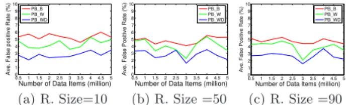
(c) R. Size =90 Figure 12: Ave. False Positive Rate of Range Queries processing time and the false positive rates.We denote the

average query result size as “R.Size” in the figures. Fig-ure 9 and FigFig-ure 10 show the average prefix query processing times and false positive rates, respectively, on different data sets, for prefix queries issued on the corresponding P B B,

P B WandP B W Dstructures. Figure 7(a) and Figure 7(b)

show the average query processing time and false positive rates, respectively, for different prefix query result sizes, on

theP B B,P B W andP B W Dstructures, which are built

on 5 million data items.

TheP B W D structure exhibits higher query processing

efficiency and records lower false positive among all PBtree structures. From the figures, we note that, for the same the query result sizes,P B W Dexecutes, 2.153, 2.309, and 2.533 times faster thanP B B, respectively; and the corresponding false positive rates inP B W Dare, 0.88, 0.8, and 0.83 times, smaller than in P B B. In comparison, for the same query result sizes, P B W executes 0.516, 0.406, and 0.444 times faster thanP B B, respectively; and the corresponding false positive rates in P B W are, 0.25, 0.186, and 0.21 times, smaller thanP B B.

6.3.2 Range Query Evaluation

Compared with existing schemes, our experimental results show thatP B W Dhas smaller range query processing times and lower false positive rates. We compared the speed of

P B W Dwith two plain text schemes:linear search, in which

we examine each item from the unsorted data set to match the range query, andbinary search, in which we execute the range query over the sorted data using the binary search algorithm. To evaluate the accuracy ofP B W D, we com-pared the recorded false positive rates with those observed in thebucket scheme of [26]. In our experiments, both the data items and the queries follow uniform distribution and hence, each bucket contains same number of data items with bucket sizes ranging from 10 to 90.

Figure 11 and Figure 12 show the average range query processing time and the false positive rates, respectively for different query result sizes on the experimental data sets. We observed that, for the three query result sizes, the plan-text binary search is, respectively, 116, 113, and 110 times, faster than the corresponding search results on theP B W D struc-ture. On the other hand,P B W Dperforms, 14.8, 3.3, and 1.748 times, faster query processing than the linear search scheme. Note, we use logarithmic coordinates in Figure 11

and Figure 8(a).

In terms of accuracy P B W D outperforms the bucket scheme [26] by orders of magnitude. For instance, for the maximum query result size of 90 in our experiments, the false positive rates recorded by P B W D are, 2.12, 21.38, and 39.96 times lesser than the bucket scheme with respec-tive bucket sizes being 10, 50, and 90.

Finally, Figure 8(a) and Figure 8(b) show the average range query processing time and false positive rates, respec-tively, for different query result sizes, where the correspond-ing indexes, P B W D, linear, binary and bucket, are built on a data set of 5 million data items.

7. CONCLUSIONS

In this paper, we propose the first range query processing scheme that achieves index indistinguishability, under the IND-CKA [19], which provides strong privacy guarantees. The key novelty of this paper is in proposing the PBtree data structure and associate algorithms for PBtree construction, searching, and optimization. We implemented and evaluated our scheme on a real world data set. The experimental re-sults show that our scheme can efficiently support real time range queries with strong privacy protection.

8. ACKNOWLEDGEMENTS

This work is supported in part by the National Natural Science Foundation of China under Grant Numbers 61370226, 61472184, 61321491, 61272546, Young Teacher Growth Plan of Hunan University, China Postdoctoral Science Founda-tion, and the National Science Foundation under Grant Num-bers CNS-1017598. We would like to thank our anonymous reviewers for their valuable suggestions and feedback for improving our paper significantly. We also like to thank Mustafa Canim and Murat Kantarcioglu for providing us the source code of their work in [26].

9. REFERENCES

[1] Amazon web services, aws.amazon.com. [2] Google app engine, code.google.com/appengine. [3] Microsoft azure, www.microsoft.com/azure. [4] Google fires engineer for privacy breach.

http://www.cnet.com/news/google fired engineer for privacy breach/, 2010.