Effective PCA for high-dimension,
low-sample-size data with noise reduction via
geometric representations
著者
Yata Kazuyoshi, Aoshima Makoto
journal or
publication title
Journal of multivariate analysis
volume
105
number
1
page range
193-215
year
2012-02
権利
(C) 2011 Elsevier Inc.
NOTICE: this is the author's version of a work
that was accepted for publication in Journal
of Multivariate Analysis. Changes resulting
from the publishing process, such as peer
review, editing, corrections, structural
formatting, and other quality control
mechanisms may not be reflected in this
document. Changes may have been made to this
work since it was submitted for publication. A
definitive version was subsequently published
in Journal of Multivariate Analysis, Vol.105
Issue 1, Pages:193-215. doi:
10.1016/j.jmva.2011.09.002
URL
http://hdl.handle.net/2241/114069
Effective PCA for high-dimension, low-sample-size data
with noise reduction via geometric representations
Kazuyoshi Yataa, Makoto Aoshima,a,1
aInstitute of Mathematics, University of Tsukuba, Ibaraki 305-8571, Japan
Abstract
In this article, we propose a new estimation methodology to deal with PCA for high-dimension, low-sample-size (HDLSS) data. We first show that HDLSS datasets have dif-ferent geometric representations depending on whether aρ-mixing-type dependency appears in variables or not. When the ρ-mixing-type dependency appears in variables, the HDLSS data converge to an n-dimensional surface of unit sphere with increasing dimension. We pay special attention to this phenomenon. We propose a method called the noise-reduction methodology to estimate eigenvalues of a HDLSS dataset. We show that the eigenvalue esti-mator holds consistency properties along with its limiting distribution in HDLSS context. We consider consistency properties of PC directions. We apply the noise-reduction methodology to estimating PC scores. We also give an application in the discriminant analysis for HDLSS datasets by using the inverse covariance matrix estimator induced by the noise-reduction methodology.
Key words: Consistency; Discriminant analysis; Eigenvalue distribution; Geometric representation; HDLSS; Inverse matrix; Noise reduction; Principal component analysis.
1. Introduction
The high-dimension, low-sample-size (HDLSS) data situation occurs in many areas of modern science such as genetic microarrays, medical imaging, text recognition, finance,
Email address: [email protected](Makoto Aoshima)
chemometrics, and so on. The asymptotic studies of this type of data are becoming in-creasingly relevant. The asymptotic behavior of eigenvalues of the sample covariance matrix in the limit asd → ∞was studied by Johnstone [6], Baik et al. [2] and Paul [10] under Gaus-sian assumptions, and Baik and Silverstein [3] under non-GausGaus-sian but i.i.d. assumptions when the dimension d and the sample size n increase at the same rate, i.e. n/d → c > 0. In recent years, substantial work has been done on the HDLSS asymptotic theory, where only d → ∞ while n is fixed, by Hall et al. [5], Ahn et al. [1], Jung and Marron [7], and Yata and Aoshima [14], [15] and [16]. Hall et al. [5] and Ahn et al. [1] explored condi-tions to give a geometric representation of HDLSS data. Jung and Marron [7] investigated consistency properties of both eigenvalues and eigenvectors of the sample covariance matrix in the HDLSS data situations. The HDLSS asymptotic theory had been created under the assumption that either the population distribution is normal or the random variables in the sphered data matrix have the ρ-mixing dependency (see Bradley [4]). However, Yata and Aoshima [14], [15] and [16] developed the HDLSS asymptotic theory without assuming either the normality or the ρ-mixing condition. Yata and Aoshima [14] gave consistency proper-ties of both eigenvalues and eigenvectors of the sample covariance matrix together with PC scores. Yata and Aoshima [15] proposed a method for dimensionality estimation of HDLSS data, and Yata and Aoshima [16] generalized the method to create a new PCA called the cross-data-matrix methodology.
In this paper, suppose we have a d×n data matrix X(d) = [x1(d), ...,xn(d)] with d > n,
where xj(d) = (x1j(d), ..., xdj(d))T, j = 1, ..., n, are independent and identically distributed
(i.i.d.) as a d-dimensional distribution with mean zero and nonnegative definite covariance matrix Σd. The eigen-decomposition of Σd is Σd = HdΛdHTd, where Λd is a diagonal
matrix of eigenvalues λ1(d) ≥ · · · ≥ λd(d)(> 0) and Hd = [h1(d), ...,hd(d)] is a matrix of
corresponding eigenvectors. Then,Z(d) =Λ− 1/2
d H T
dX(d)is a d×nsphered data matrix from
a distribution with the identity covariance matrix. Here, we write Z(d) = [z1(d), ...,zd(d)]T
and zj(d) = (zj1(d), ..., zjn(d))T, j= 1, ..., d. Hereafter, the subscript dwill be omitted for the
of each variable in Z are uniformly bounded. We assume that ||zj|| ̸= 0 for j = 1, ..., d,
where || · ||denotes the Euclidean norm. We consider a general setting as follows:
λi =aidαi (i= 1, ..., m) and λj =cj (j =m+ 1, ..., d). (1)
Here, ai(> 0), cj(> 0) and αi(α1 ≥ · · · ≥ αm > 0) are unknown constants preserving the
order that λ1 ≥ · · · ≥λd, andm is an unknown non-negative integer. We assumen > m.
In Section 2, we show that HDLSS datasets have different geometric representations depending on whether aρ-mixing-type dependency appears in variables or not. When theρ -mixing-type dependency appears in variables, the HDLSS data converge to ann-dimensional surface of unit sphere with increasing dimension. We pay special attention to this phe-nomenon. After Section 3, we assume that zjk, j = 1, ..., d (k = 1, ..., n) are independent.
Note that the assumption includes the case that X is Gaussian. In Section 3, we propose a method calledthe noise-reduction methodology to estimate eigenvalues of a HDLSS dataset. We show that the eigenvalue estimator holds consistency properties along with its limiting distribution in HDLSS context. In Section 4, we consider consistency properties of PC di-rections. In Section 5, we apply the noise-reduction methodology to estimating PC scores. In Section 6, we show performances of the noise-reduction methodology by conducting simu-lation experiments. In Section 7, we provide an inverse covariance matrix estimator induced by the noise-reduction methodology. Finally, in Section 8, we give an application in the discriminant analysis for HDLSS datasets by using the inverse covariance matrix estimator.
2. Geometric representations
In this section, we consider several geometric representations. The sample covariance matrix is S = n−1XXT. We consider the n× n dual sample covariance matrix defined
by SD = n−1XTX. Let ˆλ1 ≥ · · · ≥ ˆλn ≥ 0 be the eigenvalues of SD. Let us write the
eigen-decomposition of SD as SD =
∑n
j=1λˆjuˆjuˆ
T
j. Note that SD and S share non-zero
that when the eigenvalues of Σare sufficiently diffused in the sense that ∑d i=1λ 2 i (∑di=1λi)2 →0 as d → ∞, (2)
the sample eigenvalues behave as if they are from a scaled identity covariance matrix. When
X is Gaussian or the components of Z are ρ-mixing, it follows that
n
∑d i=1λi
SD →In (3)
in probability as d→ ∞ for a fixedn under (2).
Remark 1. The concept of ρ-mixing was first developed by Kolmogorov and Rozanov [8]. See Bradley [4] for a clear and insightful discussion. See also Jung and Marron [7]. For −∞ ≤ J ≤ K ≤ ∞, let FJK denote that theσ-field of events generated by the random variables (Yi,J ≤i≤K). For anyσ-filedA, letL2(A) denote the space of square-integrable,
Ameasurable (real-valued) random variables. For eachr≥1, define the maximal correlation coefficient
ρ(r) = sup|corr(f, g)|, f ∈L2(F−∞j ), g ∈L2(Fj∞+r),
where sup is over all f, g and j is a positive integer. The sequence {Yi} is said to be ρ
-mixing if ρ(r) → 0 as r → ∞. Note that when (z1k, z2k, ...) is ρ-mixing, it holds that for
j, j′ = 1,2, ... with |j−j′|=r,
|E((zjk2 −1)(zj2′k−1) )
| ≤ρ(r)→0 asr→ ∞.
Remark 2. Let Rn = {en ∈ Rn : ||en|| = 1}. Let wj = (n/
∑d
i=1λi)SDuˆj =
(n/∑di=1λi)ˆλjuˆj. When X is Gaussian or the components of Z are ρ-mixing, it holds
from (3) that
wj ∈Rn, j = 1, ..., n (4)
in probability as d→ ∞ for a fixedn under (2).
When X is non-Gaussian withoutρ-mixing, Yata and Aoshima [15] claimed that
n
∑d i=1λi
in probability as d → ∞ for a fixed n under (2), where Dn is a diagonal matrix with any
diagonal element having Op(1).
Now, let us further consider the geometric representations given by (3) and (5). Let
zk∗ = (z12k−1, ..., zdk2 −1)T, k = 1, ..., n. We denote the covariance matrix ofzk∗ byΦ. Note
that whenX is Gaussian (orzjk,j = 1, ..., d(k = 1, ..., n) are independent), Φis a diagonal
matrix. Let Φ = (ϕij) and r =|i−j|. Note that when the components of Z are ρ-mixing,
it holds that ϕij → 0 as r → ∞. When X is non-Gaussian without ρ-mixing, we may
claim that ϕij ̸= 0 for i̸=j. However, it should be noted that the geometric representation
given by (3) is still claimed even in a case when X is non-Gaussian withoutρ-mixing. Let us write Dk = ( ∑d j=1λj)−1 ∑d j=1λjzjk2 as a diagonal element of (n/ ∑d j=1λj)SD. Note that
Dk = ||xk||2/tr(Σ) and E(Dk) = 1. Let V(x) denote the variance of a random variable x.
We have for the variance of each Dk that
V(Dk) = E ( (∑dj=1λj(z2jk−1)) 2) (∑dj=1λj)2 = ∑ i,jλiλjϕij (∑dj=1λj)2 .
Hence, we consider a regular condition of ρ-mixing-type dependency given by ∑
i,jλiλjϕij
(∑dj=1λj)2
→0 as d→ ∞. (6)
Note that it holds (6) under (2) whenX is Gaussian or the components of Z are ρ-mixing. Then, we obtain the following theorem.
Theorem 1. When the components of Z satisfy the condition given by (6), we have (3) as
d→ ∞ for a fixed n. Otherwise, we have (5) as d→ ∞ for a fixed n under (2).
Remark 3. We consider the case that zjk, j = 1, ..., d (k = 1, ..., n) are distributed as
continuous distributions. Letf(Dk) be the p.d.f. ofDk. Assume thatZ does not satisfy (6).
Assume further that f(Dk) < ∞ w.p.1 as d → ∞. Let Rn∗ = {e(1) = (1,0, ...,0)T,e(2) =
(0,1, ...,0)T, ...,e(n) = (0,0, ...,1)T}. Then, we have that
ˆ
in probability as d→ ∞ for a fixedn under (2).
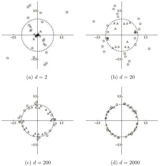
Let us observe geometric representations induced by (3) with (4) and (5) with (7). Now, we consider an easy example such as λ1 = · · · = λd = 1 and n = 2. Note that it is
satisfying (2). Figs. 1(a), 1(b), 1(c) and 1(d) give scatter plots of 20 independent pairs of ±wj (j = 1,2) generated from the normal distribution, Nd(0,Id), with mean zero and
covariance matrixId ind(= 2,20,200, and 2000)-dimensional Euclidian space, respectively.
(a) d= 2 (b) d= 20
(c) d= 200 (d) d= 2000
Fig. 1. Gaussian toy example for n= 2, illustrating the geometric representation of w1 (plotted
as⃝) andw2 (plotted as△), and the convergence to ann-dimensional surface of unit sphere with
Fig. 1 shows the geometric representation induced by (3) with (4). When d = 2, the plots of w1 appeared quite random and the plots of w2 appeared around 0. However, when
d = 200, the approximation in (3) with (4) became quite good. It reflected that the plots of wi (i = 1,2) appeared around the surface of an n-dimensional unit sphere. As expected,
when d= 2000, it showed an even more rigid geometric representation.
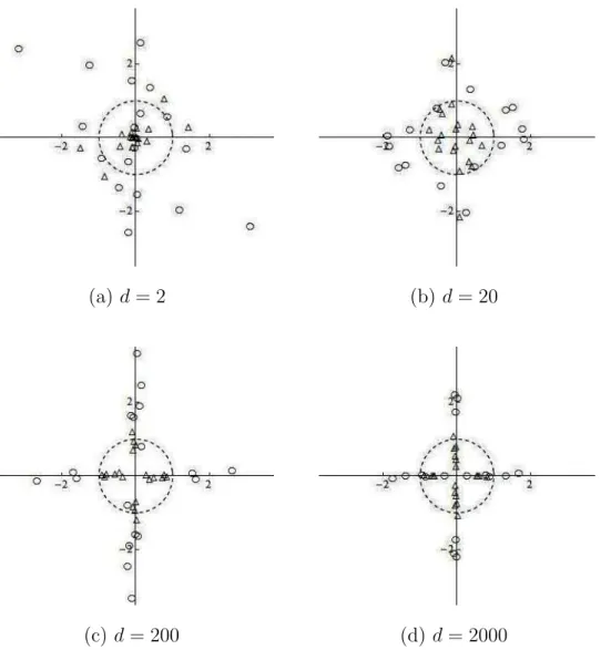
Figs. 2(a), 2(b), 2(c) and 2(d) give scatter plots of 20 independent pairs of±wj (j = 1,2)
generated from the d-variate t-distribution, td(0,Id, ν) with mean zero, covariance matrix
Id and degree of freedom (d.f.) ν = 5 in d (= 2,20,200, and 2000)-dimensional Euclidian
space.
(a) d= 2 (b) d= 20
(c) d= 200 (d) d= 2000
(plotted as ⃝) and w2 (plotted as △), and the concentration on axes with increasing dimension:
(a)d= 2, (b) d= 20, (c)d= 200, and (d) d= 2000.
Fig. 2 shows the geometric representation induced by (5) with (7). When d = 2, the plots of wi (i = 1,2) appeared quite random. When d = 200, the approximation in (5) with (7)
became moderate. Whend= 2000, the approximation became quite good. It reflected that the plots of wi (i= 1,2) appeared in close to axes.
Here, we consider the case that d → ∞ and n → ∞. Let en be an arbitrary element of
Rn that is defined in Remark 2. Then, we have the following theorem.
Theorem 2. We assume that
n ∑ i,jλiλjϕij (∑dj=1λj)2 →0 and n2 ∑p i=1λ 2 i (∑dj=1λj)2 →0 (8)
when d→ ∞ and n → ∞. Then, it holds that
n
∑d i=1λi
eTnSDen= 1 +op(1). (9)
From Theorem 2, ˆλj’s are mutually equivalent under (8) in the sense that n(
∑d i=1λi)−
1ˆλ
j =
1+op(1) for allj = 1, ..., n. Note thatn/d→0 under (8). Theorem 2 claims that a geometric
representation appeared in Fig. 1 still remains even when n→ ∞ in the HDLSS context. In this article, we pay special attention to the geometric representation given by (3) or (9), that is appeared in Fig. 1. After Section 3, we assume thatzjk, j = 1, ..., d (k = 1, ..., n)are
independent. This assumption is milder than that the population distribution is Gaussian. We propose a new estimation method called the noise-reduction methodology to deal with PCA in HDLSS data situations. When X may have the geometric representation given by (5), Yata and Aoshima [16] proposed a different method called the cross-data-matrix methodology. We compare those two methodologies by simulations in Section 6.
3. Noise-reduction methodology
by n(d) only when n = dγ, where γ is a positive constant. Yata and Aoshima [14] gave
consistency properties of the sample eigenvalues. Their result is summarized as follows: It holds for j (= 1, ..., m) that
ˆ
λj
λj
= 1 +op(1) (10)
under the conditions:
(YA-i) d→ ∞ and n→ ∞ for j such that αj >1;
(YA-ii) d→ ∞ and d1−αj/n(d)→0 forj such thatα
j ∈(0,1].
The condition described by both d→ ∞ and n → ∞ is a mild condition for n in the sense that one can choose n free from d. The above result given by Yata and Aoshima [14] draws our attention to the limitations of the capabilities of naive PCA in HDLSS data situations. Let us see a case, say, that d = 10000, λ1 =d1/2 and λ2 = · · ·= λd = 1. Then, we observe
from (YA-ii) that one requires the sample of size n >> d1−α1 = d1/2 = 100. It is somewhat inconvenient for the experimenter to handle HDLSS data situations.
We have that SD = n−1
∑d
j=1λjzjz
T
j. Let us write that U1 = n−1
∑m j=1λjzjz T j and U2 = n−1 ∑d
j=m+1λjzjzTj so that SD = U1 +U2. Here, we consider U1 as intrinsic part
and U2 as noise part. Since it holds that
∑d j=m+1λ 2 j (∑dj=m+1λj)2 →0 as d → ∞, (11)
the noise part holds the geometric representation similar to (3) or (9). Leten = (e1, ..., en)T
be an arbitrary element of Rn that is defined in Remark 2. Then, from (3) and Theorem 2,
we have that
n
∑d
j=m+1λj
eTnU2en= 1 +op(1) (12)
as d→ ∞ either when n is fixed or n=n(d) satisfying n(d)∑dj=m+1λ2
j/(
∑d
j=m+1λj)2 →0.
This geometric representation for the noise part influences the estimation scheme proposed in this article.
We consider an easy example such asm = 2 andλ1 =dα1, λ2 =dα2, λj =cj, j = 3, ..., d,
where α1 > α2 >1/2 and cj’s are positive constants. Note that it is satisfying (11). Then,
we write that λ−11SD =n−1z1zT1 + (nλ1)−1λ2z2zT2 + (nλ1)−1 ∑d j=3λjzjz T j. Let us consider the behavior of eT n(U2 −( ∑d
j=m+1λj/n)In)en in (12). By using Chebyshev’s inequality for
any τ > 0 and the uniform bound M (> 0) for the fourth moments condition, one has for all diagonal elements ofλ−11(U2−(
∑d j=m+1λj/n)In) that n ∑ i=1 P((nλ1)−1 d ∑ j=m+1 λj(zji2 −1)> τ ) ≤M τ−2n−1λ2m+1d1−2α1 =o(1) (13)
asd → ∞either whenn → ∞ornis fixed. Since we have that (nλ1)−1
∑d
j=m+1λj(zji2−1) =
op(1) for all i= 1, ..., n, it holds that all diagonal elements ofλ−11(U2−(
∑d
j=m+1λj/n)In)
converge to 0 in probability. By using Markov’s inequality for any τ > 0, one has for all off-diagonal elements of λ−11(U2−( ∑d j=m+1λj/n)In) that P( ∑ i̸=i′ ( (nλ1)−1 d ∑ j=m+1 λjzjizji′ )2 > τ ) ≤τ−1λ2m+1d1−2α1 =o(1).
Thus we have that ∑i̸=i′((nλ1)−1
∑d j=m+1λjzjizji′) 2 =o p(1) so that ∑ i̸=i′ eiei′ d ∑ j=m+1 (nλ1)−1λjzjizji′≤ ( ∑ i̸=i′ ( (nλ1)−1 d ∑ j=m+1 λjzjizji′ )2)1/2 =op(1). (14)
Then, we obtain that λ−11eTn(U2 −(
∑d
j=m+1λj/n)In)en = op(1) as d → ∞ either when
n→ ∞ orn is fixed. Note thatλ−11λ2 →0 asd→ ∞ and||n−1/2z1||= 1 +op(1) asn→ ∞.
Hence, by noting that max
en (eTnSDen) = ˆuT1SDuˆ1, it holds that λ−11uˆT1 ( SD−n−1 d ∑ j=m+1 λjIn ) ˆ u1 = ˆ uT1U1uˆ1 λ1 +op(1) = ( ˆuT1z1/n1/2)2+op(1) = 1 +op(1).
Hence, we claim as d→ ∞ and n → ∞that
λ−11 ( ˆ uT1SDuˆ1−n−1 d ∑ j=m+1 λj ) = ˆ λ1−n−1 ∑d j=m+1λj λ1 = 1 +op(1).
From the proof of Corollary 4 and Theorem 6 in Appendix, we can obtain thatn−1/2zT
1uˆ2 =
op(dα2−α1) as d → ∞ and n → ∞. By noting that ||n−1/2z2|| = 1 +op(1) as n → ∞, we
have that λ−21 ( ˆ uT2SDuˆ2 −n−1 d ∑ j=m+1 λj ) = ˆuT2 λ1z1z T 1 λ2n ˆ u2 + ˆuT2 z2zT2 n uˆ2 +op(1) = 1 +op(1).
Now, we consider estimating the noise part from the fact that as d→ ∞ and n → ∞ λ−j1 ( tr(SD)− ∑j i=1λˆi n−j −n −1 d ∑ i=m+1 λi ) =op(1)
for j = 1,2. (See Lemma 7 in Appendix for the details.) Then, we have as d → ∞ and
n→ ∞ that λ−j1 ( ˆ λj − tr(SD)− ∑j i=1λˆi n−j ) = 1 +op(1)
for j = 1,2. Hence, we have a consistent estimator for λj = dαj with αj > 1/2 that is a
milder condition than (YA-ii).
In general, we propose the new estimation methodology as follows: [Noise-reduction methodology] ˜ λj = ˆλj− tr(SD)− ∑j i=1λˆi n−j (j = 1, ..., n−1). (15)
Note that ˜λj ≥0 (j = 1, ..., n−1) w.p.1 for n ≤d. Then, we claim the following theorem.
Theorem 3. For j = 1, ..., m, we have that
˜
λj
λj
= 1 +op(1)
under the conditions:
(i) d→ ∞ and n → ∞ for j such that αj >1/2;
(ii) d→ ∞ and d1−2αj/n(d)→0 for j such that α
j ∈(0,1/2].
Theorem 4. LetV(z2
jk) = Mj (<∞)forj = 1, ..., m(k = 1, ..., n). Assume thatλj (j ≤m)
(i) d→ ∞ and n → ∞ for j such that αj >1/2;
(ii) d→ ∞ and d2−4αj/n(d)→0 for j such that α
j ∈(0,1/2], we have that √ n Mj ( ˜ λj λj −1 ) ⇒N(0,1),
where “⇒” denotes the convergence in distribution and N(0,1) denotes a random variable distributed as the standard normal distribution.
Remark 4. Yata and Aoshima [14] gave the asymptotic normality of ˆλj’s. Under the
assumption that λm+1 =· · ·=λd= 1, Lee et al. [9] considered an estimate ofλj such as
˙ λj = ˆ λj+ 1−η+ √ (ˆλj + 1−η)2−4ˆλj 2 ,
where d/n → η ≥ 0 and n → ∞. If 1/λˆj = op(1), we claim that ˙λj = (ˆλj −η)(1 +op(1)).
By noting that n−1∑dj=m+1λj → η when λm+1 = · · · = λd = 1, it holds that ˙λj = (ˆλj −
n−1∑d
j=m+1λj)(1 +op(1)). Hence, we may consider ˙λj as a noise reduction. However, we
emphasize thatthe noise-reduction methodology allows users to have a consistent estimator,
˜
λj, when λm+1 ≥ · · · ≥λd (>0) and λj =cj (j =m+ 1, ..., d) are unknown constants.
Remark 5. When X is Gaussian, α1 > 1/2 and either when α1 > α2 orm = 1, we have
as d→ ∞that ˜ λ1 λ1 ⇒ χ2 n n
for fixed n, whereχ2n denotes a random variable distributed as theχ2 distribution with d.f.
n. Jung and Marron [7] claimed a similar result for ˆλj with αj >1.
Remark 6. Whenzjk,j = 1, ..., d(k = 1, ..., n) are not independent but the components of
Z are ρ-mixing, we can claim the assertions similar to Theorems 3-4 under the conditions: (i) d→ ∞ and n→ ∞ for j such that αj >1;
(ii) d→ ∞,n → ∞ and d2−2αj/n(d)<∞ forj such thatα
The conditions (i)-(ii) are milder than the ones given by Theorem 3.1 in Yata and Aoshima [14] for a non-ρ-mixing case.
Corollary 1. When the population mean may not be zero, let us write that SoD =
(n−1)−1(X−X)T(X −X), where X = [¯xn, ...,x¯n] is having d-vector ¯xn =
∑n
s=1xs/n.
We redefine ˜λj (j = 1, ..., m) in (15) by replacing SD and n with SoD and n−1. Then, the
assertions in Theorems 3-4 are still justified under the convergence conditions.
4. Consistency properties of PC directions.
In this section, we consider PC direction vectors. Jung and Marron [7], and Yata and Aoshima [14] studied consistency properties of PC direction vectors in the context of naive PCA. Let ˆH = [ˆh1,· · · ,hˆd] such that ˆH
T
SHˆ = ˆΛ and ˆΛ= diag(ˆλ1,· · · ,ˆλd). Note that ˆhj
can be calculated by ˆhj = (nλˆj)−1/2Xuˆj, where ˆuj is an eigenvector ofSD. Then, Yata and
Aoshima [14] gave consistency properties of the sample eigenvectors with their population counterparts: Assume thatλj (j ≤m) has multiplicity one asλj ≠ λj′ for allj′(̸=j). Then,
the firstm sample eigenvectors are consistent in the sense that Angle(ˆhj,hj)
p
−→0 (j = 1, ..., m)
under (YA-i)-(YA-ii). The following result can be obtained as a corollary of Theorem 4.1 in Yata and Aoshima [14].
Corollary 2. The first m sample eigenvectors are inconsistent in the sense that Angle(ˆhj,hj)
p
−→π/2 (j = 1, ..., m) (16) under the condition that d→ ∞ and d/(n(d)λj)→ ∞.
Remark 7. Under the condition described above, we have that ˆhTjhj =op(1) (j = 1, ..., m).
Jung and Marron [7] gave (16) as d→ ∞ for a fixedn.
Remark 8. When the population mean may not be zero, we still have Corollary 2 by using
5. PC scores with noise-reduction methodology
In this section, we apply the noise-reduction methodology to principal component scores (Pcss). The j-th Pcs of xk is given by hTjxk = zjk
√
λj (= sjk, say). However, since hj
is unknown, one may use ˆhj = (nλˆj)−1/2Xuˆj as a sample eigenvector. The j-th Pcs of
xk is estimated by ˆh T
jxk = ˆujk
√
nˆλj (= ˆsjk, say), where ˆujT = (ˆuj1, ...,uˆjn). Let us define
a sample mean square error of the j-th Pcs by MSE(ˆsj) = n−1
∑n
k=1(ˆsjk −sjk)
2. Then,
Yata and Aoshima [14] evaluated the sample Pcs as follows: Assume that λj (j ≤ m) has
multiplicity one. Then, it holds that
MSE(ˆsj)
λj
=op(1) (17)
under (YA-i)-(YA-ii).
Now, we modify ˆsjk by using ˜λj defined by (15). Let us write that ˆujk
√
nλ˜j (= ˜sjk, say).
Then, we obtain the following result.
Theorem 5.Assume that λj (j ≤m) has multiplicity one. Then, we have that
M SE(˜sj)
λj
=op(1) (18)
under the conditions (i)-(ii) of Theorem 3.
For ˆuj, we can claim the consistency for a Pcs vectorn−1/2zj.
Corollary 3. Assume that λj (j ≤ m) has multiplicity one. Then, the j-th sample
eigen-vector is consistent in the sense that
Angle( ˆuj, n−1/2zj) p
−→0 (19)
under the conditions (i)-(ii) of Theorem 3.
Remark 9. Lee et al. [9] gave a result similar to (19). Under the assumption that
n→ ∞ that |uˆTjzj/n1/2|= √ 1−(λ η j−1)2 +op(1) when λj >1 +η, op(1) when 1< λj ≤1 +η.
Here, it holds that |uˆTjzj/n1/2|= 1 +op(1) underη/(λj−1)2 =O(d1−2αj/n)→0. Then, by
noting that ||zj/n1/2|| = 1 +op(1) as n → ∞, we have (19) under the conditions (i)-(ii) of
Theorem 3. Thus their result corresponds to Corollary 3 when λm+1 =· · ·=λd= 1.
Let xnew be a new sample from the distribution and independent of X. The j-th Pcs
of xnew is given by hTjxnew (= sj(new), say). Note that V(sj(new)/
√
λj) = 1. We consider a
consistent estimator of sj(new). Then, we have the following result.
Corollary 4. Assume that λj (j ≤m) has multiplicity one. For hˆj, it holds that
ˆ hTjxnew √ λj = s√j(new) λj +op(1)
under the conditions that (i) d → ∞ and n → ∞ for j such that αj > 1, (ii) d → ∞ and
d1−αj/n(d) → 0 for j such that α
j ∈ (1/3,1], and (iii) d → ∞ and d2−4αj/n(d) → 0 for j
such that αj ∈(0,1/3],
Remark 10. Lee et al. [9] also considered a predict Pcs for sj(new) when λm+1 = · · · =
λd = 1.
Now, we consider applying the noise-reduction methodology to the PC direction vectors. Let us define ˜hj = (n˜λj)−1/2Xuˆj. Then, we consider ˜hj as an estimate of the PC direction
vector, hj. By using ˜hj, j = 1, ..., m, we have the following the theorem.
Theorem 6. Assume that λj (j ≤m) has multiplicity one. For h˜j, it holds that
˜ hTjxnew √ λj = s√j(new) λj +op(1)
Remark 11. Assume that λj (j ≤ m) has multiplicity one. Then, the j-th sample
eigenvector is consistent in the sense that ˜
hTjhj = 1 +Op(n−1) +Op(d1−2αjn−1)
under the conditions (i)-(ii) of Theorem 3. For the norm, it holds that ||h˜j|| = 1 +op(1)
under (YA-i)-(YA-ii).
Remark 12. When the population mean may not be zero, we still have the above results by using SoD defined in Corollary 1.
6. Performances of noise-reduction methodology
When we observe naive PCA, the sample size n should be determined depending on d
for αi ∈ (0,1] in (YA-ii). On the other hand, the noise-reduction methodology allows the
experimenter to choose n free from d for the case that αi > 1/2 as seen in the theorems
given in Sections 3 and 5. The noise-reduction methodology is promising to give feasible estimation for HDLSS data with extremely small order of n compared tod. In this section, we examine its performance with the help of Monte Carlo simulations.
Independent pseudo-random normal observations were generated from Nd(0,Σ) with
d= 1600. We considered λ1 =d4/5, λ2 =d3/5, λ3 =d2/5 and λ4 =· · ·=λd = 1 in (1). We
used the sample of sizen∈[20,120] to define the data matrixX :d×nfor the calculation of
SD. The findings were obtained by averaging the outcomes from 2000 (=R, say) replications.
Under a fixed scenario, suppose that the r-th replication ends with estimates ofλj, ˆλjr and
˜
λjr (r= 1, ..., R), given by using (10) and (15). Let us simply write ˆλj =R−1
∑R
r=1λˆjr and
˜
λj =R−1
∑R
r=1λ˜jr. We considered two quantities, A: ˆλj/λj and B: ˜λj/λj. Fig. 3 shows the
behaviors of both A and B for the first three eigenvalues. By observing the behavior of A, (10) seems not to give a feasible estimation within the range of n. The sample size n was not large enough to use the eigenvalues of SD for such a high-dimensional space. On the
other hand, in view of the behavior of B, (15) gives a reasonable estimation surprisingly well for such HDLSS datasets. The noise-reduction methodology seems to perform excellently as
expected theoretically.
(a) For the first eigenvalue (b) For the second eigenvalue
(c) For the third eigenvalue
Fig. 3. The behaviors of A: ˆλj/λj and B: ˜λj/λj for (a) the first eigenvalue, (b) the second
eigenvalue and (c) the third eigenvalue when the samples, of size n= 20(20)120, were taken from Nd(0,Σ) withd= 1600.
We also considered the Monte Carlo variability. Let Var(ˆλj/λj) = (R−1)−1
∑R r=1(ˆλjr− ˆ λj)2/λ2j and Var(˜λj/λj) = (R−1)−1 ∑R r=1(˜λjr−λ˜j) 2/λ2
j. We considered two quantities, A:
Var(ˆλj/λj) and B: Var(˜λj/λj), in Fig. 4 to show the behaviors of sample variances of both
(a) For the first eigenvalue (b) For the second eigenvalue
(c) For the third eigenvalue
Fig. 4. The behaviors of A: Var(ˆλj/λj) and B: Var(˜λj/λj) for (a) the first eigenvalue, (b) the
second eigenvalue and (c) the third eigenvalue when the samples, of sizen= 20(20)120, were taken from Nd(0,Σ) withd= 1600.
By observing the behaviors of the sample variances, both the behaviors seem not to make much difference between A and B. Note that it holds Mj = 2 (j = 1, ..., m) for
Gaus-sian X. From Theorem 3.2 given in Yata and Aoshima [14], the limiting distribution of (n/2)1/2(ˆλj/λj − 1) is N(0,1), so that the variance of A is approximately given by
Var(ˆλj/λj) = 2/n. On the other hand, in view of Theorem 4, the limiting distribution
of (n/2)1/2(˜λj/λj − 1) is N(0,1). Hence, the variance of B is approximately given by
Var(˜λj/λj) = 2/n; that is approximately equal to the variance of A.
Next, we considered the Pcs. Independent pseudo-random normal observations were generated from Nd(0,Σ). We considered the case that λ1 = d4/5, λ2 = d3/5 λ3 =d2/5 and
λ4 =· · ·=λd= 1 in (1) as before. We fixed the sample size asn = 60. We set the dimension
MSE(ˆsj)r and MSE(˜sj)r (r = 1, ..., R), given by using (17) and (18). Let us simply write
MSE(ˆsj) = R−1
∑R
r=1MSE(ˆsj)r and MSE(˜sj) = R−1
∑R
r=1MSE(˜sj)r. We considered two
quantities, A: MSE(ˆsj)/λj and B: MSE(˜sj)/λj, in Fig. 5 to show the behaviors of both A
and B for the first three Pcss.
(a) For the first Pcs (b) For the second Pcs
(c) For the third Pcs
Fig. 5. The behaviors of A: MSE(ˆsj)/λj and B: MSE(˜sj)/λj for (a) the first Pcs, (b) the second
Pcs and (c) the third Pcs when the samples, of size n = 60, were taken from Nd(0,Σ) with
d= 800(200)1800.
Again, the noise-reduction methodology seems to perform much better than naive PCA. We conducted simulation studies for other settings as well and verified the superiority of the noise-reduction methodology to naive PCA in HDLSS data situations.
Finally, we compare the noise-reduction methodology with the cross-data-matrix ology. Yata and Aoshima [16] gave a Pcs estimator by using the cross-data-matrix method-ology. Let ´sjk be the j-th Pcs estimator of xk given in Section 5 in Yata and Aoshima [16].
td(0,Σ, ν) with mean zero, covariance matrix Σ and d.f. ν ∈ [20,80]. We considered
λ1 =d4/5, λ2 =d3/5, λ3 =d2/5 and λ4 =· · ·=λd= 1 in (1). We set d = 1600 and n = 60.
We considered three quantities, A: MSE(ˆsj)/λj, B: MSE(˜sj)/λj and C: MSE(´sj)/λj, in Fig.
6 to show the behaviors of A, B and C for the first three Pcss.
(a) For the first Pcs (b) For the second Pcs
(c) For the third Pcs
Fig. 6. The behaviors of A: MSE(ˆsj)/λj, B: MSE(˜sj)/λj and C: MSE(´sj)/λj for (a) the first
Pcs, (b) the second Pcs and (c) the third Pcs when the samples, of size n= 60, were taken from td(0,Σ, ν) withν = 20(10)80.
Note that td(0,Σ, ν) ⇒ Nd(0,Σ) as ν → ∞. When ν is small, X has the geometric
rep-resentation given by (5). In the case, the cross-data-matrix methodology seems to perform better than the noise-reduction methodology. On the other hand, whenνis large,X has the geometric representation given by (3). In the case, the noise-reduction methodology seems to perform best among the three estimators.
7. Inverse covariance matrix estimator
In this section, we apply the noise-reduction methodology to estimating the inverse covari-ance matrix of Σ. The inverse covariance matrix,Σ−1, is the key to constructing inference procedures in many statistical problems. However, it should be noted that S−1 does not exist in the HDLSS context. Srivastava [11] and [12] used the Moore-Penrose inverse of S
for several inference problems. Srivastava and Kubokawa [13] proposed an empirical Bayes inverse matrix estimator of Σ for the discriminant analysis and compared the performance with that of the Moore-Penrose inverse or the inverse matrix defined by only diagonal el-ements of S. Then, they concluded that the discriminant rule using the empirical Bayes inverse matrix estimator was better than the others. The empirical Bayes inverse matrix estimator was defined by S−δ1 = (S+δId)−1 with δ = tr(S)/n. Then, let us consider the
eigen-decomposition of S−δ1 as S−δ1 = n ∑ j=1 (ˆλj +δ)−1hˆjhˆ T j +δ−1 ( Id− n ∑ j=1 ˆ hjhˆ T j ) . Let Vδ = (vij(δ)) = Λ1/2HTS−δ1HΛ 1/2
, where Λ1/2 = diag(λ11/2, ..., λ1d/2). Note that Λ1/2HTΣ−1HΛ1/2 = Id. Let us write κ = n−1
∑d
i=m+1λi. Then, we obtain the
follow-ing result.
Theorem 7. Assume that n = n(d), α1 < 1−γ/2, γ < 1 and the first m population eigenvalues are distinct as λ1 > · · · > λm. Under the condition that (i) d → ∞ and
κ/λj =O(d1−γ−αj)<∞ for j = 1, ..., m, we have that
vjj(δ) =
2λj
λj+ 2κ
+op(1),
vjj′(δ) =op(1), j′ =j+ 1, ..., d.
For j such that λj/κ→0 as d→ ∞, we have as d→ ∞ that
vjj(δ)=λjκ−1+op(λjκ−1),
Let jδ be the maximum integer j(≤ m) such that αj −1 + γ > 0. We assume that
αj−1 +γ ̸= 0 (j = 1, ..., m). We observe that (v11(δ), ..., vjδjδ(δ), vjδ+1jδ+1(δ), ..., vdd(δ)) is close to (2, ...,2, λjδ+1κ−
1, ..., λ
dκ−1). One should note that Vδ is far from Id, so that HTS−δ1H
is far fromΛ−1. Let us consider a different inverse matrix estimator ofΣby using the noise-reduction methodology. Let ω = min(tr(S)/(d1/2n1/4), δ) and ´λ
j = max(˜λj, ω). Then, we
define a new inverse matrix estimator as
S−ω1 = n−1 ∑ j=1 ´ λ−j1h˜jh˜ T j +ω− 1 ( Id− n−1 ∑ j=1 ˜ hjh˜ T j ) , (20)
where ˜hj is the same one as in Theorem 6. LetVω = (vij(ω)) =Λ1/2HTS−ω1HΛ
1/2
. Then, we obtain the following theorem.
Theorem 8. Assume that n =n(d), γ < 1, α1 <min(1/2 +γ/4, 1−γ/2) and the first m population eigenvalues are distinct as λ1 > · · · > λm. Let ψ = min(n3/4κ/d1/2, κ). Under
the conditions that (i) d → ∞ and ψ/λj = O(d1/2−γ/4−αj) < ∞ for γ < 2/3, (ii) d → ∞
and ψ/λj =O(d1−γ−αj)<∞ for γ ∈[2/3,1), we have that
vjj(ω) =
1 max(1, ψ/λj)
+op(1),
vjj′(ω) =op(1), j′ =j+ 1, ..., d.
For j such that λj/ψ →0 as d→ ∞, we have as d → ∞ that
vjj(ω) =
λj
ψ +op(λj/ψ),
vjj′(ω) =op(λj/ψ), j′ =j + 1, ..., d.
Let jω be the maximum integer j(≤m) such that αj −1/2 +γ/4>0. We assume that
αj −1/2 +γ/4̸= 0 (j = 1, ..., m). We observe that (v11(ω), ..., vjωjω(ω), vjω+1jω+1(ω), ..., vdd(ω)) is close to (1, ...,1, λjω+1ψ−
1, ..., λ
dψ−1). Note thatψ < κw.p.1 whenγ <2/3. We can claim
Remark 13. It should be noted that ˆhTjS−ω1hˆj ≤ 0 w.p.1 as ˜λj/λˆj = op(1). Let ed be a
d-dimensional unit vector. Assume further in Theorem 8 that ed is a constant vector or ed
and S−ω1 are independent. Then, we claim as d→ ∞ that eT dS−
1
ω ed≥0 w.p.1.
8. Application
In this section, we apply the inverse covariance matrix estimator given by (20) to the dis-criminant analysis. Suppose that we have twod×Ni data matrices,Xi = [xi1, ...,xiNi], i= 1,2. We assume that x11, ...,x1N1 and x21, ...,x2N2 are independent and identically dis-tributed as π1 : Nd(µ1,Σ) and π2 : Nd(µ2,Σ), respectively. Let us write the
eigen-decomposition ofΣasΣ=∑dj=1λjhjhTj. We assume (1) aboutΣ. Letx0 be an observation
vector on an individual belonging to π1 or to π2. We estimate µ1, µ2 and Σ by
¯ xi =Ni−1 Ni ∑ j=1 xij i= 1,2, and S =n−1 2 ∑ i=1 Ni ∑ j=1 (xij −x¯i)(xij−x¯i)T,
where n=N1+N2−2. We assumed > n. We consider the discriminant rule based on the
maximum likelihood ratio under which we classifyx0 into π1 if
(1 +N1−1)−1(x0−x¯1)TS−1(x0−x¯1)<(1 +N2−1)− 1(x
0−x¯2)TS−1(x0−x¯2), (21)
and into π2 otherwise.
In the HDLSS context (d > n), there does not exist the inverse matrix of S. We observe from Theorems 7-8 that the inverse matrix estimator S−ω1 given by (20) is better than the empirical Bayes inverse matrix estimator S−δ1. Let us compare the performances ofS−ω1 and
S−δ1 by conducting simulation studies. LetS = (sij). DefineS−diag1 byS−
1
diag = diag(s−
1 11, ..., s−
1
dd). We considered the discriminant
rule given by applyingS−ω1,S−δ1 andS−diag1 toS−1 in (21). We examined its performance with the help of Monte Carlo simulations. We setd= 1600. We set µ1 = (1, ...,1,0, ...,0)T whose
first 80 elements are 1, and µ2 = (0, ...,0)T. We generated the datasets (x
i1, ...,xiNi), i = 1,2, by setting a common covariance matrix as Σ = (ρ|i−j|1/7), where ρ ∈ (0,1). Note
eigenvalues, (λ1, λ2, λ3, ...), of Σ were calculated as (44.88, 19.07, 13.55,...) when ρ = 0.2,
(198.05, 47.32, 29.77,...) when ρ = 0.4, and (491.78, 64.75, 37.80,...) when ρ = 0.6. We used a testing sample, x0 in (21), by generating 50 times randomly from π1 or π2. The
experiment was iterated 100 times. The correct classification was estimated by the average rate of correct classification over the 5000 iterations. Note that the standard deviation of this simulation study is less than 0.0071. We denoted the error of misclassifying an individual from π1 (into π2) and from π2 (into π1) by e1 and e2, respectively. We also considered the
correct discriminant rule (CDR) given by replacing (21) with (x0−µ1)
TΣ−1(x
0−µ1)<(x0−µ2)
TΣ−1(x
0−µ2).
In Table 1, we reported the correct classification rate, 1−e1, when (N1, N2) = (10,10)
and (20, 20). In Table 2, we reported the correct classification rates, (1−e1, 1−e2), when
(N1, N2) = (10,20) and (20, 40). When the correlation was low such asρ= 0.2, we observed
that the rule given byS−diag1 is as good as the others except CDR. This result is quite natural because Σ becomes close to a diagonal matrix as ρ → 0. As the variables were highly correlated, the rule given by S−diag1 became worse. It should be noted that the variables in actual HDLSS situations are highly correlated each other. When the correlation was high such as ρ = 0.4, 0.6, we observed that the rule given by S−ω1 was best among them. It should be noted that as the correlation between variables gets high, the first few eigenvalues ofΣtend to become extremely large. We may observe that the noise-reduction methodology effectively works for estimating eigenvalues in S−ω1.
Table 1. The correct classification rate, 1−e1, when (N1, N2) = (10,10) and (20, 20).
(N1, N2) = (10,10) ρ S−ω1 S−δ1 S−diag1 CDR 0.2 0.864 0.849 0.841 0.977 0.4 0.806 0.770 0.716 0.953 0.6 0.787 0.717 0.623 0.952 (N1, N2) = (20,20) ρ S−ω1 S−δ1 S−diag1 CDR 0.2 0.905 0.897 0.882 0.975 0.4 0.849 0.817 0.740 0.949 0.6 0.839 0.811 0.666 0.949
when (N1, N2) = (10,20) and (20, 40). (N1, N2) = (10,20) ρ S−ω1 S−δ1 S−diag1 CDR 0.2 (0.893, 0.872) (0.881, 0.860) (0.865, 0.848) (0.977, 0.973) 0.4 (0.815, 0.830) (0.783, 0.781) (0.722, 0.707) (0.950, 0.948) 0.6 (0.817, 0.814) (0.769, 0.759) (0.642, 0.636) (0.945, 0.957) (N1, N2) = (20,40) ρ S−ω1 S−δ1 S−diag1 CDR 0.2 (0.924, 0.920) (0.922, 0.913) (0.904, 0.901) (0.973, 0.974) 0.4 (0.861, 0.865) (0.837, 0.841) (0.761, 0.752) (0.949, 0.950) 0.6 (0.855, 0.856) (0.831, 0.835) (0.655, 0.663) (0.954, 0.951) A. Appendix
Throughout this section, let e1n and e2n be arbitrary elements of Rn. Let uij =
n−1∑d
s=m+1λszsizsj, U21 = U2 − diag(u11, ..., unn) and U22 = U2 − κIn, where κ =
n−1∑di=m+1λi. Suppose that α1 = · · · = αs1 > αs1+1 = · · · = αs2 > · · · > αsl−1+1 =
· · · = αsl(= αm), where l ≤ m. For every i (= 1, ..., l), let U1i = n−
1∑si
j=1λjzjzTj. Let
˜
λi1 ≥ · · · ≥ λ˜isi be eigenvalues of U1i. Let ˜uij(∈ Rn) be an eigenvector corresponding to
˜
λij (j = 1, ..., si). Then, we have the eigen-decomposition as U1i =
∑si
j=1λ˜iju˜iju˜Tij. Let
˜
zj = (||n−1/2zj||)−1n−1/2zj (j = 1, ..., d).
Proof of Theorem 1. By Chebyshev’s inequality, for any τ > 0, one has for each off-diagonal element (i′ ̸= j′) of (n/∑di=1λi)SD that P((
∑d i=1λi)− 1|∑d i=1λizii′zij′| > τ) ≤ τ−2(∑di=1λi)−2 ∑d i=1λ 2
i → 0 as d → ∞ under (2). Thus each off-diagonal element of
(n/∑di=1λi)SD converges to 0 in probability as d→ ∞ under (2). Thus we have that
n
∑d i=1λi
SD →diag (D1, ..., Dn)
in probability. Here, we have that P(|Dk−1| ≤τ) = 1−P(|Dk−1|> τ)≥1−τ−2V(Dk).
Dk, k = 1, ..., n, converge to 1 in probability. When the components of Z do not satisfy (6),
it holds that Dk has Op(1) for k= 1, ..., n. It concludes the result. 2
Proof of Theorem 2. By Chebyshev’s inequality and Markov’s inequality, for anyτ > 0, we have that P(∑i′,j′(∑di=1λi)−2( ∑d i=1λizii′zij′)2 > τ) ≤ n2τ−1( ∑d i=1λi)−2 ∑d i=1λ 2 i → 0 and ∑n k=1P(|Dk−1|> τ)≤nτ− 2V(D
k)→0 under (8). Thus, in a way to similar to (13)-(14),
it concludes the result. 2
The following lemma was obtained by Yata and Aoshima [14]. Lemma 1. It holds for j = 1, ..., m, that ||d−αjeT
1nU21||2 =op(1) under the conditions:
(i) d→ ∞ either when n→ ∞ or n is fixed for j such that αj >1/2;
(ii) d→ ∞ and there exists a positive constant εj satisfying d1−2αj/n < d−εj.
Lemma 2. It holds thatd−αjeT
1nU22e2n=op(1) (j = 1, ..., m)under (i)-(ii) of Theorem 3.
Proof. By using Chebyshev’s inequality, for any τ >0 and the uniform bound M(>0) for the fourth moments condition, one has under (i)-(ii) of Theorem 3 that
n ∑ k=1 P ( d−αj|u kk−κ|> τ ) = n ∑ k=1 P ( (ndαj)−1 d ∑ s=m+1 λs(zsk2 −1)> τ ) ≤(τ n1/2dαj)−2M ( ∑d s=m+1 λ2s ) ≤(τ n1/2dαj)−2M dλ2 m+1 =O(d 1−2αj/n) = o(1). Thus it holds that d−αj(u
kk−κ) = op(1) for every k (= 1, ..., n). Note that d1−2αi/n(d) =
d1−2α−γ. From (ii) of Theorem 3, there exists a positive constantεj satisfying 1−2α−γ <
−εj. Thus we have d1−2αj/n(d) < d−εj. We claim Lemma 1 under (i)-(ii) of Theorem 3.
Then, we obtain for j = 1, ..., m, that
d−αj(eT 1nU22e2n ) =d−αj(eT 1nU21e2n+eT1ndiag(u11−κ, ..., unn−κ)e2n ) =op(1).
Lemma 3. It holds as d→ ∞ and n → ∞ that
zTi U22zi′ =Op(d1/2) (i= 1, ..., m; i′ = 1, ..., m).
Proof. One can write that
zTi U22zi′ = n ∑ k1̸=k2 zik1zi′k2uk1k2+ n ∑ k=1 zikzi′k(ukk−κ).
We first consider the case of i =i′. Note that E(z2
ik1zik2zik3uk1k2uk1k3) = 0 (k1 ̸=k2 ̸= k3), E(z2 ik1z 2 ik2u 2 k1k2) = n −2∑d s=m+1λ2s (k1 ≠ k2), E(z2ik1z 2 ik2(uk1k1 −κ)(uk2k2 −κ)) = 0 (k1 ̸= k2) andE(z4 ik(ukk−κ)2)≤M2n−2 ∑d s=m+1λ 2
s for the uniform boundM for the fourth moments
condition. Then, for any τ >0, one has asd → ∞and n → ∞ that
P ( | ∑ k1̸=k2 zik1zik2uk1k2|> τ d 1/2)≤τ−2d−1 ∑ k1̸=k2 E(zik2 1z 2 ik2u 2 k1k2) =O(τ −2), P ( | n ∑ k=1 zik2(ukk−κ)|> τ d1/2 ) ≤τ−2n−1d−1M2 d ∑ s=m+1 λ2s =O(n−1) =o(1).
Thus it holds that
zTi U22zi =Op(d1/2) (i= 1, ..., m).
As for the case of i̸=i′, note that
P ( | ∑ k1̸=k2 zik1zi′k2uk1k2|> τ d 1/2) =O(τ−2), P ( | n ∑ k=1 zikzi′k(ukk−κ)|> τ d1/2 ) =o(1).
Therefore, we conclude the result. 2
Lemma 4. It holds as d→ ∞ and n → ∞ that
n−1/2zTi U22e1n =Op((d/n)1/2) (i= 1, ..., m).
Proof. We have that
||n−1/2zTi diag(u11−κ, ..., unn−κ)||2 = n
∑
k=1
By using Markov’s inequality, for any τ >0 and the uniform bound M(>0) for the fourth moments condition, one has as d→ ∞ and n→ ∞ that
P (∑n k=1 n−1zik2(ukk−κ)2 > τ d/n ) ≤τ−1d−1 n ∑ k=1 E(ukk−κ)2 =O(1/n) =o(1).
Thus it holds that ||n−1/2zT
i diag(u11−κ, ..., unn−κ)||=op((d/n)1/2). Next, we have that
||n−1/2zTi U21||2 = ∑ k1̸=k2 n−1z2ik1u2k1k2 + ∑ k1̸=k2 n−1zik1zik2 n ∑ k3(\k1,k2) uk1k3uk2k3, (22) where (\i, j) excludes numbers i, j. We consider the first term in (22). We have as d → ∞
and n → ∞that P(∑ k1̸=k2 n−1zik21u2k1k2 > τ d/n)≤τ−1d−1 ∑ k1̸=k2 E(u2k1k2) =O(τ−1). (23) Now, we consider the second term in (22). Note that E(u2
k1k3u 2 k2k3) = O(d 2/n4) and E(uk1k3uk2k3uk1k4uk2k4) =O(d/n 4) for k
1 ̸=k2 ̸=k3 ̸=k4. By using Chebyshev’s inequality,
we have that P ( | ∑ k1̸=k2 n−1zik1zik2 n ∑ k3(\k1,k2) uk1k3uk2k3|> τ d/n ) ≤τ−2d−2(n3E(u2k1k3u2k2k3) +n4E(uk1k3uk2k3uk1k4uk2k4)) =O(n −1 ) +O(d−1) = o(1). (24) By combining (23)-(24) with (22), it holds that ||n−1/2zTiU21|| = Op((d/n)1/2). Thus we
have that
n−1/2zTi U22e1n=n−1/2zTi (diag(u11−κ, ..., unn −κ) +U21)e1n=Op((d/n)1/2).
It concludes the result. 2
Lemma 5. Assume that the first m population eigenvalues are distinct as λ1 > · · ·> λm.
Then, it holds under (i)-(ii) of Theorem 3 that
ˆ
λj−κ
λj
=||n−1/2zj||2+Op(n−1) +Op(d1−2αjn−1), uˆTjz˜j = 1 +Op(n−1) +Op(d1−2αjn−1)