ISSN 1440-771X
Australia
Department of Econometrics and Business Statistics
http://www.buseco.monash.edu.au/depts/ebs/pubs/wpapers/December 2010
Working Paper 21/10
Bayesian Adaptive Bandwidth Kernel Density Estimation of
Irregular Multivariate Distributions
Bayesian Adaptive Bandwidth Kernel Density Estimation
of Irregular Multivariate Distributions
Shuowen Hu, D. S. Poskitt, Xibin Zhang∗
Department of Econometrics and Business Statistics, Monash University
December 2010
Abstract: Kernel density estimation is an important technique for understanding the distri-butional properties of data. Some investigations have found that the estimation of a global bandwidth can be heavily affected by observations in the tail. We propose to categorize data into low- and high-density regions, to which we assign two different bandwidths called the low-density adaptive bandwidths. We derive the posterior of the bandwidth parameters through the Kullback-Leibler information. A Bayesian sampling algorithm is presented to es-timate the bandwidths. Monte Carlo simulations are conducted to examine the performance of the proposed Bayesian sampling algorithm in comparison with the performance of the normal reference rule and a Bayesian sampling algorithm for estimating a global bandwidth. According to Kullback-Leibler information, the kernel density estimator with low-density adaptive bandwidths estimated through the proposed Bayesian sampling algorithm outper-forms the density estimators with bandwidth estimated through the two competitors. We apply the low-density adaptive kernel density estimator to the estimation of the bivariate density of daily stock-index returns observed from the U.S. and Australian stock markets. The derived conditional distribution of the Australian stock-index return for a given daily return in the U.S. market enables market analysts to understand how the former market is associated with the latter.
Keywords: conditional density; global bandwidth; Kullback-Leibler information; marginal likelihood; Markov chain Monte Carlo; S&P500 index
JEL Classification: C11; C14; C15
∗Address: Department of Econometrics and Business Statistics, Monash University, 900 Dandenong Road,
Caulfield East, VIC 3145, Australia. Telephone: +61 3 99032130. Fax: +61 3 99032007. Email: [email protected]
1 Introduction
Kernel density estimation is an important technique for understanding the distributional properties of data. It has been an accepted fact that the performance of a kernel density estimator is mainly determined by the choice of bandwidth, and only in a minor way by the choice of kernel (see for example, Izenman, 1991; Scott, 1992; Wand and Jones, 1995). In the current literature of kernel density estimation, people often choose to use a global bandwidth due to its simplicity. As a consequence, there have been large amount of investigations on the issue of global bandwidth selection (Jones, Marron and Sheather, 1996; Scott, 1992, among others). Abramson (1982a,b) proposed using variable bandwidths (or equivalently, adaptive bandwidths), where the resulting density estimator is a mixture of identical but individually scaled kernels being respectively centered at observations. Even though the importance of using adaptive bandwidths has been justified both theoretically and empirically, there has been a lack of attention on data-driven methods for estimating adaptive bandwidths for multivariate data. This paper aims to remedy this problem from a Bayesian perspective.
Let X = (X1,· · · , Xd)> denote a d-dimensional random vector with its density function
f(x) defined on Rd. Let {x
1,· · · ,xn} be a random sample drawn from f(x). The kernel density estimator of f(x) with a global bandwidth is given by (Wand & Jones, 1995)
ˆ fH(x) = 1 n n X i=1 KH(x−xi) = 1 n|H|1/2 n X i=1 K(H−1/2(x−xi)), (1)
whereKH(x) =|H|−1/2K(H−1/2x),K(·) is a multivariate kernel, andH is a symmetric and
positive definited×d matrix known as the bandwidth matrix.
The main issue of kernel density estimation is how we can choose an optimal bandwidth under a certain criterion. A majority of investigations has been focused on the selection of global bandwidth. When data are observed from multivariate normal density, where all variables are independent, and the diagonal bandwidth matrix H= diagonal(h1, h2,· · · , hd)
is used, Scott(1992) showed that the bandwidths that minimize the asymptotic mean inte-grated squared error (AMISE) is
hi =σi ½ 4 (d+ 2)n ¾1/(d+4) , (2)
fori= 1,2,· · · , d, andσiis the standard deviation of theith variate. This bandwidth selector
interesting cases the data are non-normal and variables are correlated, the NRR is often used due to its practicality. Sain, Baggerly and Scott (1994) presented a biased cross-validation bandwidth selector in multivariate setting using a diagonal bandwidth matrix, while Duong and Hazelton (2005) provided a cross-validation full bandwidth selector. Wand and Jones (1994) presented a plug-in selector for full bandwidth matrix but their technique sometime fails to produce finite bandwidths. This problem was solved by Duong and Hazelton (2003) who provided an alternative approach that always produces a finite bandwidth for bivariate density estimation.
Bayesian approaches to the estimation of bandwidth in kernel density estimation have been recently investigated. Basically, bandwidths are treated as parameters, and the likeli-hood of observations for given parameters can be approximated by the product of the leave-one-out kernel density estimator computed at all observations. Brewer (2000) presented a Bayesian sampling procedure for estimating variable bandwidths in univariate kernel density estimation. The study showed that the Bayesian method produced better performance than the so-called binning method proposed by Sain and Scott (1996). Kulasekera and Padgett (2006) discussed Bayes estimation of a global bandwidth for kernel density estimation based on univariate censored data using an asymmetric kernel. de Lima and Atuncarb (2010) de-rived a closed form of Bayes estimate of a global bandwidth matrix for multivariate kernel density estimation. Their method is an extension to Bayes estimation of bandwidth proposed by Gangopadhyay and Cheung (2002) for univariate kernel density estimation. Zhang, King and Hyndman (2006) derived the posterior density of bandwidth matrix through Kullback-Leibler information criterion and presented a Makov chain Monte Carlo (MCMC) simulation algorithm for estimating a global bandwidth matrix for multivariate kernel density estima-tion.
When a global bandwidth (matrix) is used for kernel density estimation, these bandwidth estimation methods perform well for many unimodal densities. However, they often produces unsatisfactory results for complex or irregular densities. For example, when the underlying true density has heavy tails, the estimation of a global bandwidth is heavily affected by extreme observations. Sain and Scott (1996) presented a classical example showing why the use of a global bandwidth is inappropriate in some situations. In a bimodal mixture of Gaussian densities, where two modes have an equal height but different variations, an optimal global bandwidth will under-smooth the mode with a large variation and
over-smooth the mode with a small variation. Hence, it is necessary to let the bandwidth vary across different observations. A relatively small bandwidth is needed for observations that are densely distributed, and a large bandwidth is required for observations that are sparsely distributed.
Some investigations have found that the estimation of a global bandwidth can be heavily affected by observations in tail areas. In an example presented by Jones (1990), the estimated density values of observations located in the tail area of a long-tailed density were lower than the true density values when a global bandwidth and Gaussian kernel are used. Hall (1987) argued that the estimation of a global bandwidth for data observed from a long-tailed distribution may mislead Kullback-Leibler information. In addition, several studies showed that using a global bandwidth in kernel density estimation tends to over smooth the modes (Wand and Jones, 1995; Sain, 2002). In terms of multivariate kernel density estimation, the distribution of observations becomes more and more sparse in the tail area of the underly true density as the dimension of data increases. Therefore, a large bandwidth is needed to smooth out large variations in the tail area. However, if a global bandwidth is used, large bandwidth will smooth out some important features of the modes.
Breiman, Meisel and Purcell (1977) and Abramson (1982b) proposed using different band-widths called adaptive bandband-widths, to scale different observations in the kernel density esti-mator. Such an adaptive bandwidth density estimator is given by Terrell and Scott (1992)
ˆ fS(x) = 1 n n X i=1 KH(xi)(x−xi) = 1 n n X i=1 1 |H(xi)|1/2 K¡H(xi)−1/2(x−xi) ¢ , (3)
where H(xi) is the bandwidth matrix for the sample data point xi. This density estimator is also called the sample-point estimator because the bandwidths are specific to the sample points or equivalently observations. Another type adaptive bandwidth density estimator is the balloon estimator, which allows the bandwidths to change with the estimation points. However, the balloon estimator does not integrate to one (see for example, Terrell and Scott, 1992; Sain and Scott, 1996; Sain, 2002).
The sample-point density estimator has the advantage over the balloon density estima-tor in that the former always integrates to one. The sample-point estimaestima-tor is actually a complete-adaptive estimator because it assigns different bandwidths to different data points. However, it is very difficult to estimate or choose bandwidths for a complete-adaptive density
estimator based on multivariate data. One way to reduce the difficulty level involved in such a density estimator is to apply the sample-point estimator to grouped or binned data (see for example, Sain and Scott, 1996; Sain, 2002). Such a density estimator is given as
ˆ fS(x) = 1 n m X j=1 njKH(tj)(x−tj) = 1 n m X j=1 nj |H(tj)|1/2 K¡H(tj)−1/2(x−tj) ¢ , (4)
wheremis the number of bins,nj is the number of observations in thejth bin,tj is the center
of the jth bin, and H(tj) is the bandwidth for the jth bin, for j = 1,2,· · · , m. Sain and
Scott (1996) conducted Monte Carlo simulations and showed that the binned sample-point estimator outperforms the density estimator with a global bandwidth.
The binned sample-point estimator has provided important insights in reducing the com-putation difficulty in multivariate adaptive kernel density estimation. The complete-adaptive density estimator assigns n different bandwidth matrices to n observations. If a diagonal bandwidth matrix is employed, the number of bandwidths will be n×d for d-dimensional data. However, the binned density estimator divides the observations into different bins ac-cording to their mutual distance, and then assigns a different bandwidth matrix to each bin of observations. Sain (2002) suggested using m bandwidths for a sample of n observations. However, the number of bandwidths for binned sample-point density estimator grows expo-nentially with the dimension. For example, when there are 10 bins in each dimension, the number of bandwidths to be estimated is 102 for bivariate data, and 103 for trivariate data. It means that the number of bandwidths can quickly exceed the number of observations as the dimension increases.
A major concern on the binned density estimation is how we can estimate the bandwidths. Even though the likelihood cross-validation method can be used, it is likely to encounter computing difficulties due to the large number of bandwidths. Zhang et al. (2006) proposed a Bayesian approach to bandwidth estimation for multivariate kernel density estimation. In a similar way to what they have done, we treat the bandwidths as parameters and obtain the posterior density of the parameters, in which the likelihood of data for given bandwidth parameters is obtained through Kullback-Leibler information.
Another concern on the binned density estimation is that the number of bandwidths to be estimated is large. We propose to divide the observations into two regions, namely the low-density region (LDR) and high-low-density region (HDR), and assign two different bandwidth matrices for the two regions. In this way, the number of bandwidths to be estimated is
obviously reduced. When the underlying true density has unimodal, the low-density region is actually the tail area. Intuitively, the low-density region should receive larger bandwidths than the high-density region. We call this type of kernel density estimator the tail-adaptive density estimator. We propose to derive the posterior of bandwidth parameters, from which we use Markov chain Monte Carlo (MCMC) sampling algorithms to sample these parameters. Therefore, the bandwidth parameters can be estimated.
The idea of distinguishing observations in low- and high-density regions has already been used in statistical inference based on kernel density estimation. Hartigan (1975, 1987) defined clusters of observations as regions of high density values. Hyndman (1996) presented an algorithm for computing and graphing data in the high-density. Mason and Polonik (2009) presented a comprehensive review of applications related to the issue of low- and high-density regions. Samworth and Wand (2010) presented an univariate bandwidth selection method for data in high-density regions. In this paper, we adopt the concept of grouping data into low-and high-density regions, in which we propose to assign two different blow-andwidth matrices for kernel density estimation.
We conduct Monte Carlo simulation studies to examine the performance of kernel density estimator with different choices of bandwidth, and Kullback-Leibler information is used as a criterion for such comparisons. In this Monte Carlo simulation study, we consider the issue of bandwidth estimation for univariate, bivariate and 5-dimensional density estimation. These densities are designed to have irregular shapes such as multimodal, skewness or fat-tailed. To demonstrate the performance of our proposed specification, we could examine the perfor-mance of the following competing methods for bandwidth estimation, namely the Bayesian approach to the estimation of a global bandwidth and NRR, as well as any sensible method to choose bandwidths for the binned density estimator. However, we will not consider the binned density estimator because it is highly computing extensive to choose bandwidths for high dimensional data. The simulation results show that the density estimator with different bandwidths assigned to the LDR and HDR often performs better than its competitors.
We illustrate the use of our proposed tail-adaptive density estimator by applying it to the estimation of bivariate density of two asset returns, which are the continuously compounded daily returns of the Australian Ordinary index (AOI) and S&P500 index, respectively. As the density of financial asset returns often exhibits a higher peak and heavier tails than the normal density, the proposed tail-adaptive kernel density estimator seems more relevant
for estimating asset return density than its counterpart with a global bandwidth. Such an investigation is important because most market analysts believe the U.S. stock market takes a leading role on all the other stock markets worldwide during the current global financial crisis. For example, market analysts might be interested in the probability that the AOI goes down if the S&P500 index went down overnight. With the estimated density of the bivariate index returns, we can compute similar probability values, which are of interests to market analysts.
The rest of this paper is organized as follows. In Section 2, we derive the posterior of bandwidth parameters and present an MCMC sampling algorithm to estimate bandwidths. Section 3 presents a Monte Carlo simulation study to examine the performance of the pro-posed tail-adaptive density estimator in comparison with its competitors, where various samples are generated from known univariate and bivariate densities. In Section 4, we carry out a simulation study with different samples of five-dimensional data. An application of the tail-adaptive kernel density estimator is presented in Section 5. Section 6 concludes the paper.
2 Bayesian estimation of bandwidths
2.1 Likelihood cross-validation
Kullback-Leibler information, which is a measure of the discrepancy between a density esti-mator and its true density, is defined as
dKL ³ f(x),fˆH(x) ´ = Z Rd log ( f(x) ˆ fH(x) ) f(x)dx = Z Rd log{f(x)}f(x)dx− Z Rd log{fˆH(x)}f(x)dx. (5)
As dKL(f(x),fˆH(x)) is nonnegative, an optimal bandwidth could be derived by minimizing
dKL(f(x),fˆH(x)) with respect to H (see for example, Duin, 1976). Such a minimization is
equivalent to the maximization of RRdlog{fˆH(x)}f(x)dx with respect to H. The sample measure of the second term of (5) is H¨ardle (1991)
b E lognfˆH(x) o = 1 n n X i=1 log ˆfH(xi) = 1 n n X i=1 log ( 1 n n X j=1 KH(xi−xj) ) . (6)
It has been shown that directly maximizing (6) with respect toH may encounter converging difficulties. H¨ardle (1991) suggested leaving the ith observation out of the sample when we compute the kernel estimator of f(xi). The resulting estimator is
ˆ fH,i(xi) = 1 n−1 n X j=1 j6=i |H|−1/2K¡H−1/2(x i−xj) ¢ , (7)
which is known as the leave-one-out estimator of f(xi), fori= 1,2,· · · , n. The well-known
likelihood cross-validation method for choosing bandwidths is to maximize CV(H) = 1 n n X i=1 log ˆfH,i(xi), (8)
with respect toH. Therefore, the optimal bandwidth denoted as ˆHKL, is
b
HKL = arg max
H CV(H). (9)
The name, likelihood, comes with the fact that n×CV(H) is an approximate log likelihood of {x1,x2,· · · ,xn} for given bandwidth parameters.
When a global bandwidth matrix is used for kernel density estimation, it is generally possible to derive an optimal bandwidth under the likelihood cross-validation rule. How-ever, the difficulty level of solving the maximization problem increases dramatically as the dimension of data increases. When complete-adaptive bandwidth matrices are used for ker-nel density estimation, it is impossible to derive optimal bandwidth matrices via likelihood cross-validation because the number of bandwidth parameters to be estimated will be multi-ples of the sample size. Even in the simple situation of univariate kernel density estimation, the number of bandwidth parameters is the same as the sample size.
Zhang et al. (2006) presented a Bayesian sampling approach to bandwidth estimation for multivariate kernel density estimation with a global bandwidth matrix, where bandwidths were treated as parameters, and the posterior of bandwidth parameters could be derived. In the situation of using complete-adaptive bandwidth matrices for kernel density estimation, it is technically possible to extend the above sampling algorithms to the situation of complete-adaptive multivariate kernel density estimation. However, it is really an extremely heavy burden to implement the sampling algorithm because the number of bandwidth parameters is n×d for diagonal bandwidth matrices n×d×(d+ 1)/2 for full bandwidth matrices.
The bandwidth matrix can be either a full matrix known as the full bandwidth matrix, or a diagonal matrix. Choosing a full bandwidth matrix provides useful theoretical features. However, implementation of such algorithm is often very difficult in practice, especially when complete-adaptive bandwidth matrices are used for kernel density estimation. The numer-ical result obtained by Sain (2002) shows that the estimated density using full bandwidth matrix is not smooth in low-density regions. Wand and Jones (1993) argued that the use of a diagonal bandwidth matrix is often appropriate because each variate receives different amount of smoothness. Zhang et al. (2006) indicated that when the variates are correlated, the effect of using a complete-bandwidth matrix can be achieved by applying a diagonal bandwidth matrix to pre-sphered data. In this paper, we use a diagonal bandwidth matrix in multivariate kernel density estimation and let h= (h1, h2, . . . , hd)> denote the vector of
the square roots of the diagonal elements of the bandwidth matrix. Note that h is also known as the bandwidth vector.
2.2 Posterior of bandwidth parameters
As the density of xi is unknown, we cannot obtain the exact likelihood of {x1,x2, . . . ,xn}
for given bandwidth parameters. However, Zhang et al. (2006) showed that the density of xi can be approximated by its kernel estimator based on the sample without the ith
observation. Such an estimator is called the leave-one-out density estimator given by ˆ fh,i(xi) = 1 n−1 n X j=1 j6=i K((xi−xj)./h)./h, (10)
for i = 1,2,· · · , n, where the operator “./” represents division by elements. The likelihood of {x1,x2, . . . ,xn} for given his `0(x1,x2, . . . ,xn|h) = n Y i=1 ˆ fh,i(xi). (11)
Assume that the prior of each element of his
p(hk)∝
1 1 +h2
k
, (12)
which is proportional to the Cauchy density, fork = 1,2,· · · , d. According to Bayes theorem, the posterior of h for given{x1,x2, . . . ,xn}is
π(h|x1,x2,· · · ,xn)∝ ( n Y i=1 ˆ fh,i(xi) ) × ( d Y k=1 1 1 +h2 k ) . (13)
Zhang et al. (2006) presented an MCMC sampling algorithm to samplehfrom its posterior.
2.3 Tail-adaptive kernel density estimator
The concept of grouping observations into low- and high-density regions has been discussed in many statistical problems. H¨artigan (1975, p205) defined a cluster as a high-density region that is separated from other high-density regions by low-density regions. In this paper, we are particularly interested in grouping observations into the low-density region, inside which every observation has a density value less than or equal to the density of every observation outside the region. In a different situation, Hyndman (1996) presented a definition for highest density region, and we follow his definition to define the LDR as follows.
Let α be a threshold value that determines the proportion of the low-density region relative to the whole sample space. Let L(fα) denote a subset of the sample space, so that
the (100×α)% low-density region is shown as
L(fα) = {x:f(x)≤fα},
where fα is the largest constant such that Pr{x∈L(fα)} ≤α.
Let
Ij =
½
1 if xj ∈L(fα)
0 otherwise ,
for j = 1,2,· · · , n. Let h(1) denote the bandwidth vector assigned to observations inside
L(fα), and h(0) the bandwidth vector assigned to observations outside L(fα). The kernel
density estimator is ˆ fh(1),h(0)(x) = 1 n n X j=1 ½ IjK ¡ (x−xj)./h(1) ¢ ./h(1) + (1−Ij)K ¡ (x−xj)./h(0) ¢ ./h(0) ¾ , (14)
and its leave-one-out estimator is ˆ fh(1),h(0),i(xi) = 1 n−1 n X j=1 j6=i ½ IjK ¡ (xi−xj)./h(1) ¢ ./h(1) + (1−Ij)K ¡ (xi−xj)./h(0) ¢ ./h(0) ¾ ,
fori= 1,2,· · · , n. As the bandwidth vector assigned for observations inside the low-density region is different from that assigned for observations outside this region, we call (14) the low-density adaptive kernel density estimator. As the low-density region becomes the tail area when the underlying density is unimodal, we also call (14) the tail-adaptive estimator for simplicity.
The tail-adaptive density estimator allows for assigning two different bandwidth matrices to observations inside the low- and high-density region. Note that the value of α can be chosen as either 5% or 10%. Then L(fα) can be interpreted as the subset that contains the
data in the tails of the density. Even though f(x) is unknown, fα can be approximated
through the kernel density estimator of f(x) using a global bandwidth. Given h(1) and h(0), the approximate likelihood is
`(x1,x2, . . . ,xn|h(1),h(0)) = n Y i=1 ˆ fh(1),h(0),i(xi). (15)
Assume that the prior of each bandwidth is
p(h(kl))∝ 1
1 +h(kl)×h(kl),
fork = 1,2,· · ·, d, and l = 0 and 1. The posterior ofh(1) andh(0) for given{x
1,x2, . . . ,xn} is π(h(1),h(0)|x 1,x2,· · · ,xn)∝ ( n Y i=1 ˆ fh(1),h(0),i(xi) ) × ( d Y k=1 p(h(1)k )×p(h(0)k ) ) . (16)
The posterior given by (16) is of non-standard form, and we cannot derive an analytical expression as the estimate of{h(1),h(0)}. However, we can use the random-walk Metropolis-Hastings algorithm to sample {h(1),h(0)}from (16). The sampling procedure is as follows.
1) Obtain an initial kernel density estimator with bandwidths chosen through NRR; and derive the low- and high-density regions for a given probability value α.
2) Assign initial values to h(1) and h(0), which are respectively, the bandwidth matrices given to observations within the low- and high-density regions specified in Step 1). 3) Let ˜hdenote the vector of all elements of{h(1),h(0)}. Apply the random-walk
Metropolis-Hastings algorithm to the update of ˜h with the acceptance probability computed through the posterior given by (16).
4) Derive the low- and high-density regions according the density estimator with the bandwidth matrices updated in Step 3).
5) Repeat Steps 3) and 4) until the simulated chain of ˜h achieves reasonable mixing performance.
During the above iterations, we usually discard the draws during the burn-in period, and record the draws of ˜hthereafter. Let {h˜(1),h˜(2),· · · ,h˜(M)} denote the recorded draws. The posterior mean (or ergodic average) denoted asPMi=1h˜(i)/M, is an estimate of ˜h. Once the bandwidth matrices are estimated, the analytical form of the kernel density estimator is obtained.
3 A Monte Carlo simulation study
To investigate the performance of the proposed tail-adaptive kernel density estimator, we approximate Kullback-Leibler information between the density estimator and its correspond-ing true density via Monte Carlo simulation. Kullback-Leibler information defined in (5) is a measure of discrepancy between the true density and its estimator. To approximate Kullback-Leibler information, we draw a large number of random vectors {x1,x2, . . . ,xN}
from true density f(x) and compute ˆ dKL ³ f(x),fˆ(x) ´ = 1 N N X i=1 log ³ f(xi)/fˆ(xi) ´ , (17)
where ˆf(·) denote a density estimator of f(·). The performance of a bandwidth estimate is examined through the performance of the resulting kernel density estimator. A bandwidth estimation method is better than its competitor if Kullback-Leibler information resulted from the former is less than that resulted from the latter.
3.1 True densities
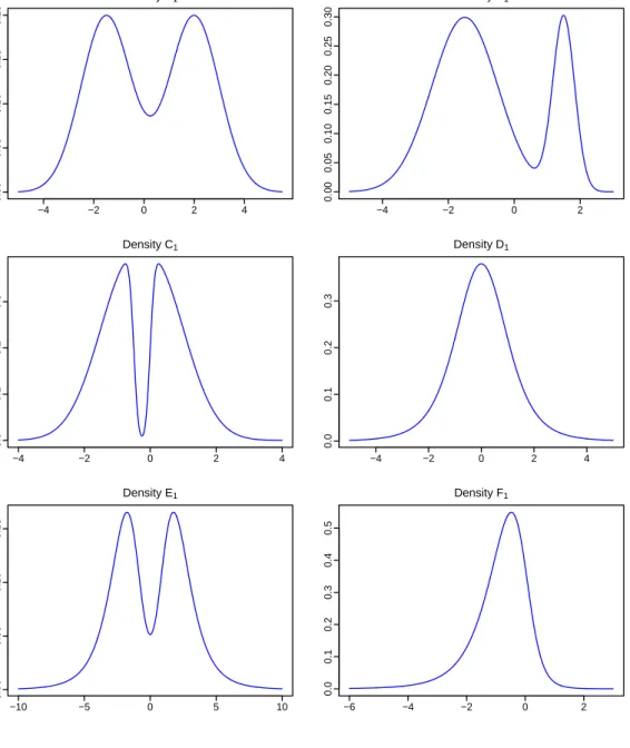
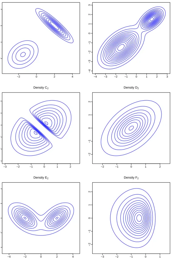
We conduct Monte Carlo simulation by simulating samples from six target densities labeled A, B, C, D, E and F, which are denoted as A1 to F1 for univariate densities, and A2 to F2 for bivariate densities. Figure 1 provides the density plot for univariate densities and Figure
2 shows the contour plot for bivariate densities. These densities are of irregular shapes. Density A and B are normal densities with bimodality. Density E and F are Student t
densities with heavy-tail features. Density C and G are skew-normal and skew-t densities, respectively. There specifications are explained as follows.
Density A is a mixture of two equally weighted normal densities with bimodality:
fA(x|µ1,Σ1, µ2,Σ2) = 1
2φ(x|µ1,Σ1) + 1
2φ(x|µ2,Σ2),
whereφ(x|µ,Σ) denotes a multivariate normal density with mean µand variance-covariance matrix Σ. The univariate true density is fA1(x) = 1/2φ(x|2,1) + 1/2φ(x| −1.5,1), while
the bivariate bivariate true density has the following mean vectors and variance-covariance matrices. µ1 = µ −1.5 −1.5 ¶ , Σ1 = µ 1 0.3 0.3 1 ¶ , µ2 = µ 2 2 ¶ , Σ2 = µ 1 −0.9 −0.9 1 ¶ .
Note that this bivariate density was used by Zhang et al. (2006).
Density B is a mixture of two normal densities with different weights but an equal height at the modes: fB(x|µ1,Σ1, µ2,Σ2) = 3 4φ(x|µ1,Σ1) + 1 4φ(x|µ2,Σ2).
The univariate density isfB1(x) = 3/4φ(x|−1.5,1)+1/4φ(x|−1.5,1/9), which was discussed
by Sain and Scott (1996). The bivariate density is the same mixture with mean vectors and variance-covariance matrices given as follows.
µ1 = µ −1.5 −1.5 ¶ , Σ1 = µ 1 1/2 1/2 1 ¶ , µ2 = µ 1.5 1.5 ¶ , Σ2 = µ 1/3 1/6 1/6 1/3 ¶ .
Density C is a mixture of two skew-normal densities:
fC(x|µ1, γ1, µ2, γ2,Σ) =0.5×2φ(x|µ1,Σ)Φ ¡ γ1>(x−µ1) ¢ +0.5×2φ(x|µ2,Σ)Φ ¡ γ2>(x−µ2) ¢
where Φ(·) is the cumulative density function of a multivariate standard normal distribution, and γ1, γ2 ∈ Rd are the shape parameters determining the skewness. This distribution was proposed by Azzalini and Valle (1996) and the conventional normal density can be obtained whenγ1 =γ2 = 0. The univariate densityfC1 has the following parameter values: µ1 =−0.5, µ2 = 0, α1 =−9 and α2 = 9. The bivariate density has the following parameters values:
µ1 = µ −0.5 −0.5 ¶ , α1 = µ −9 −9 ¶ , µ2 = µ 0 0 ¶ , α2 = µ 9 9 ¶ , Σ = µ 1 0.3 0.3 1 ¶ .
Density D is a Student t distribution denoted as td(x|µ,Σ, ν): fD(x|µ,Σ, ν) = Γ((ν+d)/2) (νπ)d/2Γ(ν/2)|Σ|1/2 · 1 + 1 ν(x−µ) 0Σ−1(x−µ) ¸−(d+ν)/2 , (18)
which has the location parameterµ, dispersion matrix Σ and degrees-of-freedom ν= 5. The parameter vector of the univariate densityfD1(x) is (0,1,5)
>, while bivariate densityf
D2(x)
has the following parameters:
µ= µ 0 0 ¶ , Σ = µ 1 0.5 0.5 1 ¶ .
Density E is a mixture of two Student t densities with degrees of freedom ν= 5:
fE(x|µ1, µ2,Σ, ν) = 0.5 td(x|µ1,Σ1, ν) + 0.5 td(x|µ2,Σ2, ν).
The univariate densityfE1(x) = 0.5t1(x| −2,1,5) + 0.5t1(2,1,5), and the bivariate density fE2(x) = 0.5t2(x|µ1,Σ1,5) + 0.5 t2(µ2,Σ2,5), where µ1 = µ −2 0 ¶ , Σ1 = µ 1 −0.5 −0.5 1 ¶ , µ2 = µ 2 0 ¶ , Σ2 = µ 1 0.5 0.5 1 ¶ .
Density F is a skew-t density proposed by Azzalini and Capitanio (2003):
fF(x|µ,Σ, α, ν) = 2 td(x|µ,Σ, ν)Td( ˜x|ν+d), (19) where ˜ x=γ>ω−1(x−µ) µ ν+d (x−µ)>Σ−1(x−µ) +ν ¶1/2 ,
ω is a diagonal matrix with diagonal elements the same as those of Σ, and Td(·|ν+d) is the
cumulative density of the Studentt distribution withν+ddegrees of freedom. The density given by (19) is able to capture heavy tailed property with ν= 5 and moderately skewness. The univariate density fF1(x) has parameters µ = 0, α = −2 and Σ = 1. The bivariate
densityfF2(x) has the following parameters:
µ= µ 0 0 ¶ , γ= µ −2 0 ¶ , Σ = µ 1 0 0 1 ¶ .
The density graph of each of the six univariate densities is presented in Figure 1, while the contour plot of each of the six bivariate densities is given in Figure 2. We can find that these densities exhibit a variety of different distributional properties.
3.2 Accuracy of our Bayesian bandwidth estimation
We generated samples of sizes n = 200,500,1000 from each of the six univariate densities, as well as samples of sizes n = 500,1000,2000 from each of the six bivariate densities. The kernel function for estimating univariate densities was chosen to be the univariate standard Gaussian density known as the Gaussian kernel, and the product of univariate Gaussian kernels was used as the kernel function for estimating multivariate densities. The bandwidth matrix in estimating multivariate densities was chosen to be a diagonal matrix.
First, we estimated the diagonal bandwidth matrices for our proposed tail-adaptive kernel density estimator with α = 0.05 and 0.1. Second, we consider the kernel density estimator with a global bandwidth (matrix), which was estimated through two existing selection or estimation methods, namely the NRR discussed by Scott (1992) and the Bayesian sampling technique presented by Zhang et al. (2006).
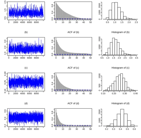
In terms of our proposed tail-adaptive density estimator used for each generated sample, we applied the random-walk Metropolis-Hastings algorithm to the update of all bandwidths in the univariate situation (or all components of the bandwidth matrices in the bivariate situation) with the acceptance probability calculated through (13). There are 3,000 iterations during the burn-in period, and the recorded period contains 10,000 iterations. We computed the batch-mean standard deviation discussed by Roberts (1996) and the simulation inefficient factor (SIF) discussed by Kim, Shepherd and Chib (1998) to monitor the mixing performance (or loosely speaking, the convergence performance). Both indicators are explained in details in Zhang et al. (2006). As the simulated chain is a Markov chain, the SIF value can be roughly interpreted as the number of draws needed so as to produce independent draws. Therefore, a small SIF value usually indicate good mixing performance. In addition, a plot of the sample path of each parameter, together with its autocorrelation function (ACF) and histogram graphs is also presented for visual inspection of the mixing performance.
Consider a sample generated from fF2(x) with the probability of the low-density region α = 0.05 and sample size n = 1000. Figure 3 presents graphs of the sample path, its ACF and histogram of each bandwidth. Table 1 presents a summary of the MCMC results, in which we found that the SIF values are very small, and the batch-mean standard deviations are respectively, much smaller than their counterparts of overall standard deviations. These
indicators show that the mixing performance of the proposed sampling algorithm applied to the tail-adaptive kernel density estimator is very good and acceptable.
The estimates of bandwidths are also sensible. Note that fF2 is a fat-tailed density with
left skewness in one dimension and a certain degree of symmetry in the other dimension (see Figure 2). We found that the tail-adaptive density estimator clearly captures the fat-tailed feature of the true density. For example, the estimates of both components ofh(1) for observations inside the low-density region are respectively, much larger than the estimates of both components of h(0) for observations outside this region.
In order to examine the performance of the proposed tail-adaptive density estimator with different bandwidth matrices assigned to the low- and high-density regions, we also derived global bandwidths (or bandwidth matrices for the bivariate situation) through the NRR and the Bayesian sampling method. However, we do not report the estimated bandwidths, but the resulting Kullback-Leibler information.
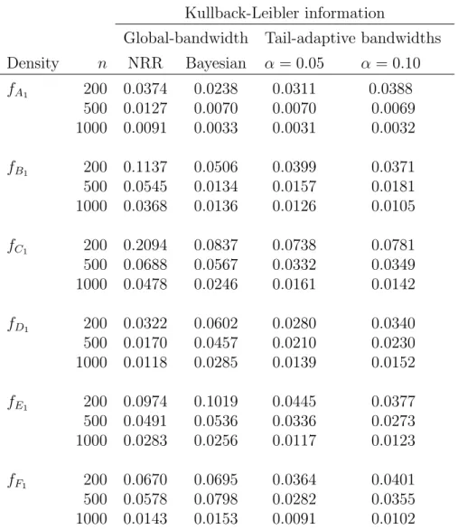
We generated N=100,000 random numbers (or vectors for the bivariate situation) from the true density and calculated the estimated Kullback-Leibler information defined by (17). For the six univariate densities, Table 2 presents the estimated Kullback-Leibler information between the true density and each density estimator resulted from each bandwidth estima-tion method. Among all six densities considered, the tail-adaptive density estimator with bandwidths estimated through Bayesian sampling and low-density probability 0.05 clearly performs better than the global-bandwidth estimator with bandwidth selected through NRR; and the former clearly performs better than the global-bandwidth estimator with bandwidth estimated through Bayesian sampling except DensityA1. When the Bayesian estimation of a global bandwidth performs worse than the NRR of a global bandwidth for Densities D1 toF1, our proposed Bayesian estimation of tail-adaptive bandwidths outperforms the NRR. Table 2 also shows that there is no obvious difference between different choices of α, which is the probability of the low-density region.
The estimated Kullback-Leibler information for bivariate densities is given in Table 3. Among all six densities considered, the tail-adaptive density estimator obviously performs better than global-bandwidth density estimator with bandwidth matrix estimated through either the NRR or Bayesian sampling. Note that Bayesian estimation of a global bandwidth matrix performs slightly worse than NRR in the case of fF2 with sample size 500, our
proposed Bayesian estimation of tail-adaptive bandwidth performs clearly better than the two competitors. The results also indicate that the performance of the tail-adaptive density estimator is not very sensitive to different values of the probability of low-density region.
4 Tail-adaptive density estimation for high dimensions
Our proposed Bayesian sampling algorithm for estimating bandwidths (or bandwidth matri-ces in multivariate situations) in tail-adaptive kernel density estimation is applicable to data of any dimension. In this section, we aim to examine the performance of the tail-adaptive es-timator with bandwidth matrices estimated through Bayesian sampling in comparison with its two competitors, namely the NRR and Bayesian estimation of a global bandwidth matrix proposed by Zhang et al. (2006).4.1 True densities
We consider four target densities labeled G, H, I and J. Density G is a mixture of two multivariate normal densities:
fG(x|µ1, µ2,Σ1,Σ2) = 1
2φ(x|µ1,Σ1) + 1
2φ(x|µ2,Σ2),
with location parameter vectors specified as µ1 = (−1.5,−1.5,−1.5,−1.5,−1.5)> and µ2 = (2,2,2,2,2)> and both variance-covariance matrices of the form
Σ = 1 1−ρ2 1 ρ ρ2 ρ3 ρ4 ρ 1 ρ ρ2 ρ3 ρ2 ρ 1 ρ ρ2 ρ3 ρ2 ρ 1 ρ ρ4 ρ3 ρ2 ρ 1 , (20)
where ρ= 0.3 for Σ1 and ρ=−0.9 for Σ2.
Density H is a multivariate skew-normal densities:
fH(x|µ,Σ, α) = 2φ(x|µ,Σ) Φ
¡
γ>(x−µ)¢,
where Σ is defined by (20) withρ= 0.9,µ= (−0.5,−0.5,−0.5,−0.5,−0.5)>, Φ(·) is the
Density I is a mixture of two multivariate Student t densities:
fI(x|µ1, µ2,Σ1,Σ2, ν) = 0.5td(x|µ1,Σ1, ν) + 0.5td(x|µ2,Σ2, ν),
where µ1 = (−2,0,−2,0,−2)>, µ2 = (2,0,2,0,2)>, ν = 5, and both Σ1 and Σ1 are defined by (20) with ρ=−0.5 and ρ= 0.5, respectively.
Density J is a multivariate skew-t densities:
fJ(x|µ,Σ, α, ν) = 2td(x|µ,Σ, ν)Td(x˜|ν+d),
where µ = 0, ν = 5, Σ is a d× d identity matrix, and x˜ is defined by (19) with γ = (2,0,2,0,2)>.
4.2 Accuracy of our Bayesian bandwidth estimation
We generated samples of sizesn= 500,1000,2000 from each of the five-dimensional densities. Table 4 presents the estimated Kullback-Leibler information between the true density and its estimator resulted from each of the three bandwidth estimation methods. We found that our proposed Bayesian estimation of the tail-adaptive bandwidth matrix obviously outperforms the NRR for choosing a global bandwidth matrix in kernel density estimation. Moreover, we found that the former clearly performs better than Bayesian estimation of a global bandwidth matrix. These findings are consistent with what we found in the bivariate situation.
For all sample sizes of each density considered, we found that the tail-adaptive kernel density estimator with α = 0.1 slightly outperforms the same estimator with α = 0.05. However, we would be reluctant to make a decision as to whether the former performs better than the latter because such a difference resulted from the two different probability values is marginal.
5 An application of the tail-adaptive density estimator
In this section, we apply the proposed tail-adaptive kernel density estimator to the estimation of bivariate density of stock-index returns. We obtained the daily closing index values of the S&P500 index in the U.S. stock market and the All Ordinaries Index (AOI) in the Australianstock market, where the sample period is from the 2nd January 2006 to the 16th September 2010 excluding non-trading days. In the finance literature, most researchers believe that the density of financial asset returns has a higher peak and heavy tails than the normal density. If a global bandwidth is used for kernel density estimator, the use of a global bandwidth is likely to over-smooth the density due to the existence of observations in the tail areas. The use of complete-adaptive bandwidths may not be attractive in application due to the large number of bandwidth parameters. Therefore, we wish to apply the tail-adaptive kernel density estimator to the estimation of bivariate-return density.
Letxt denote the closing index at datet. The daily continuously compounded returns in
percentage form was computed as (lnxt−lnxt−1)×100. The sample size isn = 1155. The sample period is an important period because it contained some extremely volatile observa-tions caused by the current global financial crisis. Table 5 presents some basic descriptive statistics. We found that both return series have mean values around zero, a certain degree of negative skewness and excessive kurtosis. As shown in the scatter plot of the bivariate observations given in Figure 4, the daily returns of both indices are correlated with the Pearson correlation coefficient 0.6171. We can visually identify many extreme return values in Figure 4, which indicates that the joint density of the bivariate index returns has very heavy tails during the sample period.
We used our Bayesian sampling algorithm to estimate bandwidths matrices for the tail-adaptive kernel density estimator of the bivariate index returns, where the probability of low-density region was chosen to be 5%. We also applied the Bayesian sampling algorithm proposed by Zhang et al. (2006) and NRR to the estimation of global bandwidth matrix for the kernel estimation of the bivariate return density.
There were 3,000 iterations in burn-in period and 10,000 iterations in the recorded period for both sampling algorithms. Table 6 presents a summary of the results, where the batch-mean standard deviation and SIF measures indicate very good mixing performance of both samplers. Moreover, we calculated the log marginal likelihood of Newton and Raftery (1994) for each of the two density estimators so as to decide which is favored against the other. The log marginal likelihood for our tail-adaptive kernel density estimator is -1657.14, which is obviously larger than -1719.64, the log marginal likelihood for the global-bandwidth kernel density estimator. Thus, we have found strong evidence supporting our tail-adaptive density estimator against the global-bandwidth density estimator.
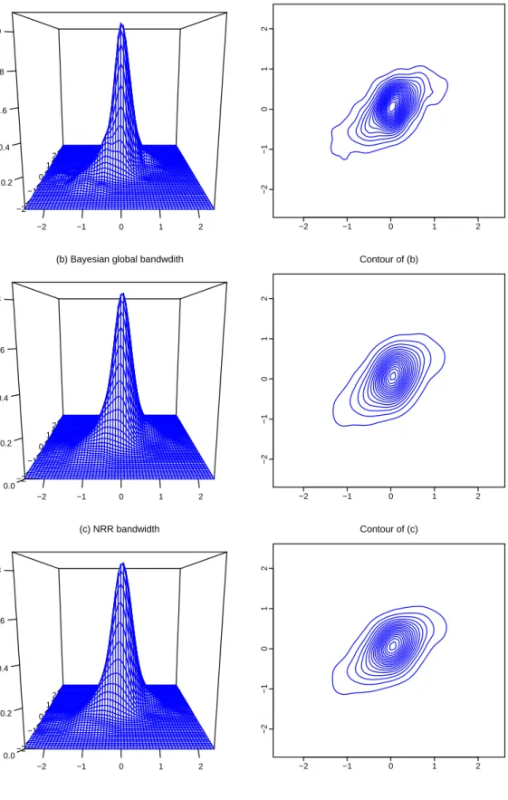
With the estimated tail-adaptive bandwidth matrices given in the 3rd column of Table 6, we calculated the tail-adaptive density estimator of the bivariate index returns, whose density surface and contour graph presented in the 1st row of Figure 5. Moreover, the 2nd row of Figure 5 presents the same set of graphs produced by the global bandwidth matrix estimated via the Bayesian sampling algorithm of Zhang et al. (2006). The last row of Figure 5 presents the same set of graphs produced by the global bandwidth matrix estimated via NRR. Both the density surface and the contour produced via the tail-adaptive estimator is obviously different from those produced via each global-bandwidth density estimator. Both the density surface of contour plot of the tail-adaptive density estimator show that this estimator captures richer dynamics than the other two density estimators.
Let xt denote the S&P500 index return and yt the AOI return. We used the bandwidth
matrices estimated through our tail-adaptive density estimator to estimate the conditional density of AOI return given that the S&P500 return equals a certain value. Such a conditional density is expressed as
f(y|xt=x) =
f(y, x)
fx(x)
,
wheref(y, x) is the joint density of (yt, xt), and fx(x) is the marginal density of xt.
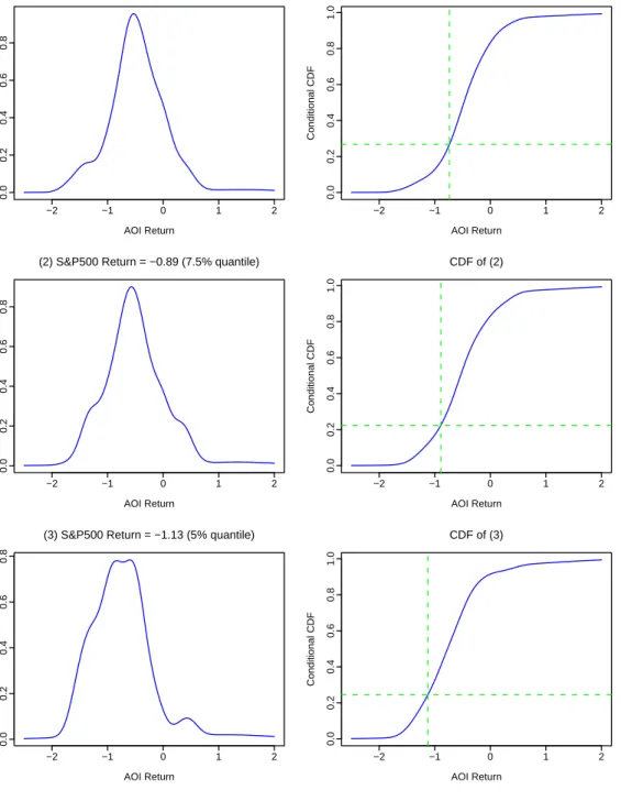
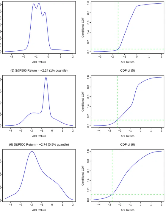
Accord-ing to Holmes, Gray and Isbell Jr (2010) and Polak, Zhang and KAccord-ing (2010), bandwidths estimated through a joint density can also be used for the purpose to compute conditional density. As market analysts are often concerned with the left tail of the density of stock-index returns, we computed the conditional density of AOI returns given that the S&P500 return is at each of the quantiles of 10%, 7.5% 5%, 2.5%, 1% and 0.5%, which are corresponding to percentage return values of -0.73, -0.89, -1.13, -1.52, -2.24 and -2.74, respectively. The graph of each conditional density is presented in the 1st columns of Figure 6 and Figure 7, from which we can visually understand the distributional properties of the AOI return given that the U.S. stock market finished daily trading with the S&P500 index return at a certain value.
With the tail-adaptive bandwidth matrices estimated via our Bayesian sampling algo-rithm, we are able to estimate the conditional probability of the form
Pr{yt≤y|xt≤x}= Pr{yt≤y, xt≤x}
Pr{xt≤x}
. (21)
Such a calculation can be done simply by replacing the Gaussian kernel with its cumulative density function. The interpretation of (21) is also clear and meaningful to market analysts.
Given that the U.S. stock market went down beyondx%, the probability that the Australian stock market would drop beyond y% is approximated through (21). We found that Pr{yt≤
0|xt ≤ 0} = 0.67. It means that when the U.S. stock market finished daily trading with a
negative return, there was a 67% chance that the Australian stock market would also drop. Given that such a chance is more than 50%, we could say that the Australian stock market followed the U.S. stock market during the global financial crisis.
With the tail-adaptive kernel density estimator estimated through our Bayesian sampling algorithm, we are able to estimate the conditional cumulative density function (CDF) of yt
for given xt=x: F(y|xt=x) = Pr{yt ≤y|xt=x}= Z y −∞ f(z, x) fx(x) dz. (22)
The conditional CDF was estimated in the same way as we estimated f(y|xt=x) with the
Gaussian kernel function forytreplaced with the Gaussian CDF function. The interpretation
of (22) is clear and meaningful to market analysts. Given that the U.S. stock market finished daily trading with the S&P500 index return being atx%, the probability that the Australian stock market drops beyond the same daily return level is indicated by (22).
We used the above-mentioned quantiles of the S&P500 return and derived the conditional CDF values as follows. Pr{yt≤ −0.73|xt=−0.74}= 0.27, Pr{yt≤ −0.89|xt=−0.89}= 0.22, Pr{yt≤ −1.13|xt=−1.13}= 0.24, Pr{yt≤ −1.52|xt=−1.52}= 0.05, Pr{yt≤ −2.24|xt=−2.24}= 0.12, Pr{yt≤ −2.74|xt=−2.74}= 0.11. (23)
The interpretation of these values is clear. Even though the Australian stock market followed the U.S. stock market during the global financial crisis, the probability that the Australian market had a larger drop than the U.S. market was at most 27%.
Each graph in the 2nd columns of Figures 6 and 7 plots the curve of the conditional CDF function ofyt given that xt takes each of the above six values. With these graphs, we
Thus, this type of graphs is helpful for us to understand how the Australian stock market followed the U.S. stock market during the current global financial crisis.
6 Conclusion
This paper proposes a kernel density estimator with tail-adaptive bandwidths, which are assigned to the low- and high-density regions, respectively. We have derived the posterior of bandwidth parameters based on Kullback-Leibler information and presented an MCMC sampling algorithm to estimate bandwidths. The Monte Carlo simulation study shows that the kernel density estimator with tail-adaptive bandwidths estimated through our proposed Bayesian sampling algorithm outperforms its competitor, the kernel density estimator with a global bandwidth estimated through either the normal reference rule discussed in Scott (1992) or the Bayesian sampling algorithm proposed by Zhang et al. (2006). The simulation result also shows that the improvement made by the tail-adaptive kernel density estimator is especially obvious when the underlying density is fat-tailed. Even though the probability of the low-density region αhas to be chosen before we carry out the sampling procedure, we have found that performance the low-density adaptive kernel estimator is not sensitive to the changes of such probability values. Therefore, it is the users’ choice on what the probability of the low-density region should be. Future study could include such a probability value as an additional parameter to be estimated through the sampling procedure.
We applied the tail-adaptive kernel density estimator to the estimation of bivariate den-sity of the paired daily returns of the Australian Ordinary index and S&P500 index during the period of global financial crisis. The tail-adaptive density estimator captures richer dy-namics in the tail area than the density estimator with a global bandwidth estimated through the normal reference rule and a Bayesian sampling algorithm. With the tail-adaptive band-widths estimated through our proposed Bayesian sampling algorithm, we have derived the estimated conditional density and distribution of the Australian index return given that the U.S. market finished daily trading with different return values. We have found that during the global financial crisis, even though the Australian stock market followed the U.S. stock market, there was no more than 27% chance that the former market had a larger drop than the latter. The graphs of the conditional density and distribution enable market analysts to approximate various probability values conditional on the behavior of the U.S. stock market.
References
Abramson, I. S. (1982a). Arbitrariness of the pilot estimator in adaptive kernel methods.
Journal of Multivariate Analysis 12 562-567.
Abramson, I. S. (1982b). On bandwidth variation in kernel estimates-a square root law. The Annals of Statistics 10 1217-1223.
Azzalini, A. and Capitanio, A. (2003). Distributions generated by perturbation of symmetry with emphasis on a multivariate skew t-distribution. Journal of the Royal Statistical Society, Series B65 367-389.
Azzalini, A. and Valle, A. D. (1996). The multivariate skew-normal distribution. Biometrika
83 715-726.
Breiman, L., Meisel, W. and Purcell, E. (1977). Variable kernel estimates of multivariate densities. Technometrics 19 135-144.
Brewer, M. J. (2000). A Bayesian model for local smoothing in kernel density estimation.
Statistics and Computing 10 299-309.
de Lima, M. S. and Atuncarb, G. S. (2010). A Bayesian method to estimate the opti-mal bandwidth for multivariate kernel estimator. Journal of Nonparametric Statistics
doi:10.1080/10485252.2010.485200.
Duin, R. P. W. (1976). On the choice of smoothing parameters for Parzen estimators of probability density functions, IEEE Transactions on Computers 100 1175-1179.
Duong, T. and Hazelton, M. L. (2003). Plug-in bandwidth matrices for bivariate kernel density estimation. Journal of Nonparametric Statistics 15 17-30.
Duong, T. and Hazelton, M. L. (2005). Cross-validation bandwidth matrices for multivariate kernel density estimation. Scandinavian Journal of Statistics 32 485-506.
Gangopadhyay, A. and Cheung, K. (2002). Bayesian approach to the choice of smoothing parameter in kernel density estimation. Journal of Nonparametric Statistics 14655-664. Hall, P. (1987). On Kullback-Leibler loss and density estimation, The Annals of Statistics
15 1491-1519.
H¨adle, W. (1991). Smoothing Techniques: with Implementation in S. Springer, New York. Hartigan, J. A. (1975). Clustering Algorithms. John Wiley & Sons, New York.
Hartigan, J. A. (1987). Estimation of a convex density contour in two dimensions. Journal of the American Statistical Association 82 267-270.
Holmes, M. P., Gray, A. G. and Isbell Jr, C. L. (2010). Fast kernel conditional density esti-mation: A dual-tree Monte Carlo approach. Computational Statistics & Data Analysis
54 1707-1718.
Hyndman, R. J. (1996). Computing and graphing highest density regions. The American Statistician 50 120-126.
Izenman, A. J. (1991). Recent developments in nonparametric density estimation. Journal of the American Statistical Association 86 205-224.
Jones, M. C. (1990). Variable kernel density estimates and variable kernel density estimates.
Australian & New Zealand Journal of Statistics 32 361-371.
Jones, M. C., Marron, J. S. and Sheather, S. J. (1996). A brief survey of bandwidth selection for density estimation. Journal of the American Statistical Association 91 401-407. Kim, S., Shepherd, N. and Chib, S. (1998). Stochastic volatility: likelihood inference and
comparison with ARCH models. Review of Economic Studies 65 361-393.
Kulasekera, K. B. and Padgett, W. J.(2006). Bayes bandwidth selection in kernel density estimation with censored data. Journal of Nonparametric Statistics 18 129-143.
Mason, D. M. and Polonik, W. (2009). Asymptotic normality of plug-in level set estimates.
The Annals of Applied Probability 19 1108-1142.
Newton, M. A. and Raftery, A. E. (1994). Approximate Bayesian inference with the weighted likelihood bootstrap. Journal of the Royal Statistical Society, Series B 56 3-48.
Polak, J., Zhang, X. and King, M. L. (2010). Bandwidth selection for kernel conditional den-sity estimation using the MCMC method. Manuscript presented at Australian Statistical Conference, 6-10 December, Fremantle, Western Australia.
Roberts, G. O. (1996). Markov chain concepts related to sampling algorithms. In W. R. Gilks, S. Richardson, & D. J. Spiegelhalter (Eds.),Markov Chain Monte Carlo in practice
(pp. 45-57). Chapman & Hall, London.
Sain, S. R. (2002). Multivariate locally adaptive density estimation. Computational Statis-tics & Data Analysis 39 165-186.
Sain, S. R., Baggerly, K. A. and Scott, D. W. (1994). Cross-validation of multivariate densities. Journal of the American Statistical Association 89 807-817.
Sain, S. R. and Scott, D. W. (1996). On locally adaptive density estimation. Journal of the American Statistical Association 91 1525-1534.
Samworth, R. J. and Wand, M. P. (2010). Asymptotics and optimal bandwidth selection for highest density region estimation. The Annals of Statistics 38 1767-1792.
Scott, D. W. (1992). Multivariate Density Estimation: Theory, Practice, and Visualization.
John Wiley & Sons, New York.
Terrell, G. R. and Scott, D. W. (1992). Variable kernel density estimation. The Annals of Statistics 20 1236-1265.
Wand, M. P. and Jones, M. C.(1993). Comparison of smoothing parameterizations in bi-variate kernel density estimation. Journal of the American Statistical Association 88
520-528.
Wand, M. P. and Jones, M. C. (1994). Multivariate plug-in bandwidth selection. Computa-tional Statistics 9 97-116.
Wand, M. P. and Jones, M. C. (1995). Kernel Smoothing. Chapman & Hall, New York. Zhang, X., King, M. L. and Hyndman, R. J. (2006). A Bayesian approach to bandwidth
selection for multivariate kernel density estimation. Computational Statistics & Data Analysis 50 3009-3031.
Table 1: A summary of MCMC results obtained based on a sample generated from density F2
Bandwidths Mean Standard Batch-mean SIF Acceptance
deviation standard deviation rate
LDR adaptive h(1)1 1.1121 0.3184 0.0157 24.32 0.28
α= 0.05 h(1)2 1.6432 0.3816 0.0164 18.57
h(0)1 0.2505 0.0469 0.0019 17.13
h(0)2 0.4196 0.0675 0.0018 7.35
Table 2: Estimated Kullback-Leibler information for univariate densities
Kullback-Leibler information
Global-bandwidth Tail-adaptive bandwidths Density n NRR Bayesian α= 0.05 α= 0.10 fA1 200 0.0374 0.0238 0.0311 0.0388 500 0.0127 0.0070 0.0070 0.0069 1000 0.0091 0.0033 0.0031 0.0032 fB1 200 0.1137 0.0506 0.0399 0.0371 500 0.0545 0.0134 0.0157 0.0181 1000 0.0368 0.0136 0.0126 0.0105 fC1 200 0.2094 0.0837 0.0738 0.0781 500 0.0688 0.0567 0.0332 0.0349 1000 0.0478 0.0246 0.0161 0.0142 fD1 200 0.0322 0.0602 0.0280 0.0340 500 0.0170 0.0457 0.0210 0.0230 1000 0.0118 0.0285 0.0139 0.0152 fE1 200 0.0974 0.1019 0.0445 0.0377 500 0.0491 0.0536 0.0336 0.0273 1000 0.0283 0.0256 0.0117 0.0123 fF1 200 0.0670 0.0695 0.0364 0.0401 500 0.0578 0.0798 0.0282 0.0355 1000 0.0143 0.0153 0.0091 0.0102
Table 3: Estimated Kullback-Leibler information for bivariate densities
Kullback-Leibler information
Global-bandwidth Tail-adaptive bandwidth
Density n NRR Bayesian α= 0.05 α= 0.10 fA2 500 0.2878 0.0858 0.0772 0.0748 1000 0.2382 0.0617 0.0498 0.0467 2000 0.1981 0.0402 0.0339 0.0338 fB2 500 0.1201 0.0499 0.0444 0.0442 1000 0.0826 0.0349 0.0332 0.0337 2000 0.0653 0.0256 0.0219 0.0217 fC2 500 0.1126 0.0930 0.0783 0.0768 1000 0.0924 0.0689 0.0559 0.0558 2000 0.0900 0.0648 0.0497 0.0498 fD2 500 0.1171 0.0946 0.0464 0.0449 1000 0.0809 0.0769 0.0286 0.0312 2000 0.0590 0.0565 0.0242 0.0270 fE2 500 0.1436 0.1072 0.0623 0.0530 1000 0.1038 0.1088 0.0328 0.0397 2000 0.0782 0.0666 0.0262 0.0282 fF2 500 0.1169 0.1641 0.0520 0.0545 1000 0.0781 0.0657 0.0261 0.0306 2000 0.0708 0.0637 0.0237 0.0242
Table 4: Estimated Kullback-Leibler information for 5-dimensional densities
Kullback-Leibler information
Global-bandwidth Tail-adaptive bandwidth
Density n NRR Bayesian α= 0.05 α= 0.10 fG 500 0.8923 0.4280 0.4026 0.4004 1000 0.7705 0.3093 0.2848 0.2825 2000 0.6933 0.2489 0.2343 0.2300 fH 500 0.4559 0.3438 0.3212 0.3179 1000 0.4041 0.2892 0.2613 0.2582 2000 0.3355 0.2226 0.2033 0.1987 fI 500 0.5943 0.5674 0.3446 0.3187 1000 0.4994 0.4814 0.2891 0.2666 2000 0.4395 0.4255 0.2274 0.2072 fJ 500 0.6107 0.5755 0.3226 0.3033 1000 0.5969 0.4415 0.2538 0.2284 2000 0.5050 0.3937 0.1971 0.1773
Table 5: Some descriptive statistics of the daily continuously compounded returns of the S&P500 index and AOI
Series n Mean Standard Skewness Kurtosis Correlation
deviation
S&P500 1155 -0.0058 0.7034 -0.2197 11.1613 0.6171
AOI 1155 0.0015 0.5779 -0.3955 6.4593
Table 6: A summary of MCMC results obtained through our proposed Bayesian sampling algo-rithm to the tail-adaptive kernel density estimator of the S&P500 and AOI returns
Bandwidths Mean Standard Batch-mean SIF Acceptance log marginal deviation standard deviation rate likelihood NRR h1 0.2171 h2 0.1783 Bayesian global h1 0.1795 0.0113 0.0003 5.63 0.21 -1719.64 bandwidth h2 0.2485 0.0121 0.0003 5.89 Tail-adaptive h(1)1 0.5533 0.2217 0.0139 39.30 0.27 -1657.14 bandwidth h(1)2 0.1221 0.0161 0.0006 15.39 withα= 0.05 h(0)1 0.5552 0.1140 0.0051 19.97 h(0)2 0.1547 0.0174 0.0006 13.55
Figure 1: Density graphs of target univariate densities. −4 −2 0 2 4 0.00 0.05 0.10 0.15 0.20 Density A1 −4 −2 0 2 0.00 0.05 0.10 0.15 0.20 0.25 0.30 Density B1 −4 −2 0 2 4 0.0 0.1 0.2 0.3 Density C1 −4 −2 0 2 4 0.0 0.1 0.2 0.3 Density D1 −10 −5 0 5 10 0.00 0.05 0.10 0.15 Density E1 −6 −4 −2 0 2 0.0 0.1 0.2 0.3 0.4 0.5 Density F1
Figure 2: Contour graphs of target bivariate densities. Density A2 −2 0 2 4 −2 0 2 4 Density B2 −4 −3 −2 −1 0 1 2 3 −4 −3 −2 −1 0 1 2 3 Density C2 −3 −2 −1 0 1 2 −3 −2 −1 0 1 2 Density D2 −2 −1 0 1 2 −2 −1 0 1 2 Density E2 −4 −2 0 2 4 −4 −2 0 2 4 Density F2 −3 −2 −1 0 1 −2 −1 0 1 2
Figure 3: Plots of posterior draws obtained through our proposed sampling algorithm for
tail-adaptive bandwidths in kernel density estimation with α=0.05: (a) h(1)1 ; (b) h(1)2 ; (c) h(0)1 ; and
(d)h(0)2 . 0 2000 4000 6000 8000 0.5 1.5 2.5 (a) 0 10 20 30 40 50 0.0 0.4 0.8
ACF of (a) Histogram of (a)
0.5 1.0 1.5 2.0 2.5 0 1000 2000 0 2000 4000 6000 8000 1.0 2.0 3.0 (b) 0 10 20 30 40 50 0.0 0.4 0.8 ACF of (b) Histogram of (b) 0.5 1.0 1.5 2.0 2.5 3.0 3.5 0 1000 2000 0 2000 4000 6000 8000 0.10 0.25 0.40 (c) 0 10 20 30 40 50 0.0 0.4 0.8 ACF of (c) Histogram of (c) 0.10 0.20 0.30 0.40 0 500 1500 0 2000 4000 6000 8000 0.2 0.4 0.6 (d) 0 10 20 30 40 50 0.0 0.4 0.8 ACF of (d) Histogram of (d) 0.2 0.3 0.4 0.5 0.6 0 1000 2500
Figure 4: A scatter plot of daily continuously compounded daily returns of S&P500 and AOI in percentage form during the period from the 2nd January 2006 to 16th September 2010
−4 −2 0 2 4 −3 −2 −1 0 1 2 S&P500 return AOI return
Figure 5: Surface graphs and contour plots of the three density estimators produced by (a)
tail-adaptive bandwidths with α = 5%; (b) Bayesian global bandwidth; and (c) NRR bandwidth. In
each surface graph, the x-axis represents index return in percentage, and the y-axis represents
density. In each contours plot, both axises represent index return in percentage.
−2 −1 0 1 2 −2 −1 0 1 2 0.2 0.4 0.6 0.8 1.0
(a) Tail−adaptive bandwidth Contour of (a)
−2 −1 0 1 2 −2 −1 0 1 2 −2 −1 0 1 2 −2 −1 0 1 2 0.0 0.2 0.4 0.6 0.8
(b) Bayesian global bandwdith Contour of (b)
−2 −1 0 1 2 −2 −1 0 1 2 −2 −1 0 1 2 −2 −1 0 1 2 0.0 0.2 0.4 0.6 0.8 (c) NRR bandwidth Contour of (c) −2 −1 0 1 2 −2 −1 0 1 2
Figure 6: Each graph in the left column represents the conditional density given that the S&P500 return is at the chosen value. Each graph in right column represents the conditional CDF
com-puted through (22) at differentyvalues for a givenx value marked by the vertical line, while the
horizontal line marks the y value that is the same as the chosen x value.
−2 −1 0 1 2 0.0 0.2 0.4 0.6 0.8
(1) S&P500 Return = −0.74 (10% quantile)
AOI Return Conditional Density −2 −1 0 1 2 0.0 0.2 0.4 0.6 0.8 1.0 CDF of (1) AOI Return Conditional CDF −2 −1 0 1 2 0.0 0.2 0.4 0.6 0.8
(2) S&P500 Return = −0.89 (7.5% quantile)
AOI Return Conditional Density −2 −1 0 1 2 0.0 0.2 0.4 0.6 0.8 1.0 CDF of (2) AOI Return Conditional CDF −2 −1 0 1 2 0.0 0.2 0.4 0.6 0.8
(3) S&P500 Return = −1.13 (5% quantile)
AOI Return Conditional Density −2 −1 0 1 2 0.0 0.2 0.4 0.6 0.8 1.0 CDF of (3) AOI Return Conditional CDF
Figure 7: Each graph in the left column represents the conditional density given that the S&P500 return is at the chosen value. Each graph in right column represents the conditional CDF
com-puted through (22) at differentyvalues for a givenx value marked by the vertical line, while the
horizontal line marks the y value that is the same as the chosen x value.
−3 −2 −1 0 1 2 0.0 0.1 0.2 0.3 0.4 0.5 0.6 0.7
(4) S&P500 Return = −1.52 (2.5% quantile)
AOI Return Conditional Density −3 −2 −1 0 1 2 0.0 0.2 0.4 0.6 0.8 1.0 CDF of (4) AOI Return Conditional CDF −4 −3 −2 −1 0 1 2 0.0 0.2 0.4 0.6 0.8
(5) S&P500 Return = −2.24 (1% quantile)
AOI Return Conditional Density −4 −3 −2 −1 0 1 2 0.0 0.2 0.4 0.6 0.8 1.0 CDF of (5) AOI Return Conditional CDF −4 −3 −2 −1 0 1 2 0.0 0.1 0.2 0.3
(6) S&P500 Return = −2.74 (0.5% quantile)
AOI Return Conditional Density −4 −3 −2 −1 0 1 2 0.0 0.2 0.4 0.6 0.8 1.0 CDF of (6) AOI Return Conditional CDF