The Menstrual Cycle and Performance Feedback Alter Gender Differences in Competitive Choices

Munich Personal RePEc Archive

The Menstrual Cycle and Performance

Feedback Alter Gender Differences in

Competitive Choices

Wozniak, David and Harbaugh, William T. and Mayr, Ulrich

Eastern Michigan University, University of Oregon

August 2009

The Menstrual Cycle and Performance Feedback Alter Gender

Differences in Competitive Choices

David Wozniak2

William T. Harbaugh3

Ulrich Mayr4

March 25, 2011

1

We are grateful for support and direction from Chris Minson and Paul Kaplan of the University of Oregon Human Physiology Department. Seminar participants at the (June) 2009 ESA and (July) 2009 IAREP/SABE meetings provided useful ideas and comments. Correspondence should be addressed to David Wozniak (Eastern Michigan University) at [email protected]. We would also like to thank Jack Wozniak for his programming assistance and Cathleen Leue, the director of the Social Science Instructional Labs and her staff at the University of Oregon. A final thanks to Sarah Wunderlich for all her help scheduling and running experiments.

2

Eastern Michigan University

3

University of Oregon

4

The Menstrual Cycle and Performance Feedback

Alter Gender Differences in Competitive Choices.

March 25, 2011

Abstract

We use a within-subjects experiment with math and word tasks to show that feedback about

relative performance moves high ability females towards more competitive forms of compensation

such as tournaments, moves low ability men towards piece rate and group pay, and eliminates

gender differences in choices. We also examine choices for females across the menstrual cycle, and

find that women in the high-hormone phase are more willing to compete than women in the low

phase, though somewhat less willing to compete than men. There are no significant differences

Introduction

Economic experiments have shown when given the choice between piece rate and

winner-take-all tournament style compensation, women are more reluctant than men to choose tournaments

(e.g. Niederle and Vesterlund 2007). These gender difference experiments have all relied on a

framework where subjects were not informed of their abilities relative to potential competitors. We

use a within-subjects design and replicate these previous findings for a math task, and show they

also exist for a word task. We then show that feedback about relative performance moves high

ability females towards more competitive compensation schemes, moves low ability men towards less

competitive schemes such as piece rate and group pay, and removes the average gender difference

in compensation choices. We also examine between and within-subjects differences in choices for

females across the menstrual cycle. We find that the relative reluctance to choose tournaments on

the part of women comes mostly from women in the low-hormone phase of their menstrual cycle.

Women in the high-hormone phase are substantially more willing to compete than women in the low

phase, though still somewhat less willing to compete than men. There are no significant differences

between the choices of any of these groups after they receive relative performance feedback.

In low information settings the effects of gender and menstrual phase are large. A female has

a 0.14 lower probability of choosing a tournament compared to a male, even when controlling for

performance and confidence. For a female to be as likely to choose a tournament as an average male

she must believe she is 40% better than average in performance. We find that the within-gender

menstrual phase effect is larger than the across-gender effect. Females in the low-hormone phase of

their cycle have a 0.16 lower probability of choosing a tournament than females in high-hormone

phase. A low phase female must believe she has 50% better performance to be as likely to compete

as a female in the high-hormone phase.

Without feedback, high ability females and males are both more reluctant to enter tournaments

than expected value maximization would require. This effect is larger for high ability females. On

the other hand, too many low ability types enter competitive environments, and this effect is larger

for males. Relative performance feedback moves all these groups toward more optimal choices. This

result suggests that the behavioral differences in the willingness to compete are driven less by stable

preference differences than by differing reactions to the generally poor information concerning a

One motivation for experiments on gender differences in competitive behavior comes from the

job market where many careers involve a tournament aspect. An example of this is the corporate

ladder, where females make up a small portion of top-level executive positions. Bertrand and

Hallock (2001) found that in 1997 the fraction of females in top level management positions was

3% and only 15% of firms had at least one female in a top level executive position. There are

many potential explanations for this underrepresentation. Discrimination is one explanation, the

effect of traditional family roles and raising children on women’s career choices and human capital

investments is another (Polachek 1981). Part of this underrepresentation may be caused by a

preference by females against competitive, tournament-like situations in favor of alternatives – or

by a preference by men towards competition and tournaments.

Such a preference difference could have many causes. For example, Jirjahn and Stephan (2004)

argue that the attractiveness of piece rate schemes for females is likely caused by reduced wage

discrimination in such a setting, when performance can easily be measured. It could be for this

reason that firms with a higher proportion of females are more likely to offer piece rate compensation

(Brown 1990).

Another explanation could be a differential performance increase during competition. Gneezy,

Niederle, and Rustichini (2003) find that females see lower performance gains from participating in

competitive environments. Gneezy and Rustichini (2004) also find that this gender difference exists

at a young age; by observing children’s performance in running races, they find that competition

increases the performance of boys, but not girls. These differences in performance seem tied to

the gender of competitors. Gneezy, Niederle, and Rustichini (2003) also find that in mixed-gender

competitive environments males have significant performance increases when an environment is

made more competitive, while females do not. However, when females compete only against other

females, their performance increases as the environment becomes more competitive. Gupta, Poulsen

and Villeval (2005) find that females are more competitive when given the opportunity to choose

the gender of a potential competitor. Specifically, females are more likely to choose to enter a

tournament if they first choose to be paired against another female before making the tournament

entry decision. These results suggest that the gender composition of groups may play a role in

performance gains from competition, as well as in the selection into competitive environments.

gender difference remains large even after controlling for the relatively larger overconfidence of

men. Dohmen and Falk (2007) report similar results.

Different preferences for risk and ambiguity are another possible explanation. In most

compe-tition experiments the subjects have very little information about their relative ability when they

make their competitive choices. They typically learn their own performance in trial runs, but not

the performance of potential competitors. Grossman and Eckel (2003) provide a review of gender

differences in risk preferences and find that results generally, but not always, find that females are

more risk averse than men. However, most experimental studies examining gender differences for

competition argue that gender differences in competitive choices remain after using various controls

for risk preferences. Ambiguity aversion is also a possibility, but ambiguity aversion has not been

found to vary systematically across gender. Moore and Eckel (2003) find that females are more

ambiguity averse for specific contexts and domains, while Borghans et al. (2009) find that males

are initially more ambiguity averse than females, but as ambiguity increases, males and females

behave similarly.

None of the results cited so far show that these gender differences in competitive behavior

are biologically determined. In fact, Gneezy et al. (2009) report results from experiments in

a matrilineal society in India where women are more likely to compete than men in contrast

participants in a patriarchical society performing the same type of tasks. Such a result suggests

that socialization plays a large role in such gender differences. Cross cultural studies of this sort

are one way to isolate the effects of biological factors. In this paper, we use systematic variations

in the levels of hormones for females across the menstrual cycle to examine the same question. We

find that women’s competitive choices vary substantially across the cycle. Interestingly, the effect

is such that during the low-hormone phase of the cycle the behavioral differences are quite large,

while in the high-hormone phase females choices to compete are similar to those of males.

Hormones have been found to affect various economic behaviors in humans. The hormone

oxytocin has been found to increase trusting behavior of individuals (Baumgartner et al. 2008).

Fehr (2009) suggests that due to such results, preferences towards trust are affected by biological

mechanisms. For males, testosterone levels of financial traders in the morning can predict their

daily profits. Cortisol levels in these same traders were found to rise with increased volatility in

their market returns (Coates and Herbert 2008). Testosterone levels are correlated with behaviors

Financial risk taking has also been linked to circulating levels of testosterone in men (Apicella et

al. 2008).

Males and females have very different levels of a number of hormones, including estrogen,

luteinizing hormone (LH), follicle stimulating hormone (FSH), progesterone, and testosterone (Speroff

and Fritz 2005); however, these hormones do not necessarily have the same effects across genders.

Additionally, in a review article Shepard et al. (2009) conclude that the large literature on sex

differences and brain organization indicates that the expression of hormonal effects within a

gen-der may be very dependent on the particular environment ungen-der consigen-deration. Women exhibit

large and predictable hormonal variations across the menstrual cycle (Speroff and Fritz 2005).

For females, estrogen and progesterone have received most of the attention in studies examining

behavioral effects.1

The mechanisms by which hormones affect behaviors are explained by neuroendocrinological

research on how hormones alter brain activity. Results show that major depression may be linked

to reduced density of serotonin binding sites (Malison et al. 1998). By injecting estrogen in rats,

Fink et al. (1996) find that estrogen stimulates an increase in the density of serotonin binding sites

in certain areas of the brain, including the anterior cingulate cortex, anterior frontal cortex and

the nucleus accumbens – areas that have been linked to the anticipation and receipt of monetary

rewards (Fink et al. 1996, McEwen 2002, Bethea et al. 2002, Platt and Huettel 2008). Progesterone

has been shown to inhibit neurotransmission, and as a result it may decrease anxiety and increase

sedation (Vliet 2001). Other research suggests that progesterone may decrease the degradation

rate of serotonin (Bethea et al. 2002).

Sex differences in the brain develop during perinatal development where both females and

male brains are organized differently from different exposure to steroid hormones (Gagnidze and

Pfaff 2009). For female rodent brains, estrogen masculinizes aramatase-expressing neural pathways

and also masculinizes territorial behavior (Wu et al. 2009). Aromatase is an enzyme that converts

testosterone to estradiol. In the adult male brain testosterone acting through androgen receptors

is necessary to complement male type behavior (Gagnidze and Pfaff 2009). For females, estrogen is

required and received by estrogen receptors to express male-type aggressive and territorial behavior

in mice (Gagnidze and Pfaff 2009). Thus, estrogen for females may lead to similar behavior for

females as that induced by testosterone in males. Dreher et al. (2007) uses fMRI to assess brain

1

activity during the anticipation of uncertain money payments, across different phases of the

men-strual cycle. While the study does not include decisions, they find significant changes in activation

in areas related to the processing of rewards (such as the striatum) and in the amygdala, an area

that activates during fear and anxiety.

In this study, we exploit the large variations in estrogen and progesterone levels that occur in

females over the menstrual cycle. As shown in Figure 1, both progesterone and estrogen remain

low during the early part of the menstrual cycle. This first week of the cycle is when normal

cycling females menstruate and can be considered a low-hormone phase. The later part of this

is called the pre-follicular phase. Estrogen then rises quickly and spikes just prior to ovulation

– this is referred to as the follicular spike. After ovulation (approximately day 14 in the graph),

during what is called the luteal phase, females who ovulate experience heightened levels of both

progesterone and estrogen. This second spike in both hormones may be referred to as the luteal

spike or high-hormone phase (Speroff and Fritz 2005, Stricker et al. 2006). Testosterone levels

also vary over the menstrual cycle, peaking just before the follicular estrogen spike (Sinha-Hikim

et al. 1998). However the spike is much smaller than for estrogen, and testosterone levels are

insignificantly different during menses and the luteal spike.

Figure 1: Hormonal Fluctuations in Normal Cycling Females

Only a few studies have examined the economic effects of the menstrual cycle. Ichino and

Moretti (2009) use detailed employee attendance data from a large Italian bank and find that

absences for females below the age of 45 tend to occur according on a 28-day cycle. These 28-day

cycle absences explain about one-third of the gender gap in employment absences at the firm. The

female menstrual cycle is approximately 28 days and they focus on females below the age of 45, who

are more likely to be pre-menopausal. In an experimental study, Chen et al. (2010) explore the

possibility that menstrual cycle phase effects drive bidding differences between males and females

in auctions. They find bidding differences in first-price auctions, with females in the low hormone

follicular phase bidding more than females in the high hormone luteal phase, though most of this

variation is found to be driven by contraceptive users. In direct contrast, Pearson and Schipper

(2009) find that women bid more than men, and earn lower profits, only during the menstrual and

premenstrual phases of the cycle when estrogen and progesterone levels are lower. There is one

experimental study looking at competitive choices and the menstrual cycle, Buser (2010). This is

a between-subjects study of choices of females to compete in all-female groups, and it finds that

females participating during predicted high levels of progesterone tend to be less competitive. We

compare these results with ours in the discussion section.

Not all economic studies have found support for hormonal effects on economic decision making.

Zethraeus et al. (2009) examine 200 post-menopausal women in a double-blind study. Participants

were given either estradiol (2 mg), testosterone (40 mg), or a placebo daily for a four week period.

Then they participated in an economic experiment session that included a variety of different tasks

looking at risk aversion, altruism, reciprocal fairness, trust and trustworthiness. No significant

differences were found when comparing the behaviors between the three different treatment groups

of females. Some research shows that neural receptors in post-menopausal women may have reduced

sensitivity to hormonal changes, due to the effects of aging (Chakraborty et al. 2003). Such an

aging effect could explain the lack of differences in such a study. Ideally, we would use a

double-blind study using exogenous delivered hormones to examine the effects of hormonal differences, but

such a study is not feasible with pre-menopausal women, since low hormone levels cause bleeding

1

Experimental Design

We use a within-subjects design with sessions about 2 weeks apart. An online pre-screening survey

was used to recruit and schedule subjects for experiment sessions. We limited the sample of females

to those using a monophasic hormonal contraceptive or not using hormonal contraceptives at all.2

For normally cycling females, the sessions were scheduled during a low-hormone phase (days 2 to

7 in Figure1 ) and a high-hormone phase (days 18 to 25 in Figure1 ) of the menstrual cycle. These

high and low phases are supported by research examining a drop in hormones during menses (Aden

et al. 1998). We intentionally avoided the estradiol spike around day 14, because of its short

duration and variability within and across females. Other phases were also avoided due to greater

measurement error about the hormone changes that could be occurring during those times. Thus,

we limit our study to examining the greatest contrast in hormones for females by using a scheduling

design that has been successfully used in the field of neuroscience (Fernandez et al. 2003).

Females using a hormonal contraceptive experience suppression of endogenous hormone

pro-duction when in the active phase of their contraceptive regimen (Speroff and Fritz 2005). Both

progesterone and estrogen levels remain fairly constant as the body receives a daily dose of

hor-mones exogenously (Aden et al. 1998). During the placebo or non-active phase of the contraceptive

regimen, there are no exogenous hormones being provided to the body; this withdrawal leads to

withdrawal bleeding (Speroff and Fritz 2005). Since menstrual bleeding is caused by low hormones,

this allows for easy identification of the low-hormone phase. We scheduled contraceptive users

and normal cycling females accordingly, so that both would be in the experiment during a

low-hormone phase and during a high-low-hormone phase. The high-low-hormone phase coincides with the

luteal spike for normal cycling females and a stable elevated hormone phase for contraceptive users.

We avoided the follicular spike, because it is short and difficult to time and therefore difficult to

correctly schedule subjects into sessions.3

Using the screening survey, females were first randomly scheduled during a predicted high or

predicted low-hormone phase. Men were simply scheduled for two sessions about 2 weeks apart. To

help minimize errors in classifying phases correctly, we also used an exit survey. The low-hormone

2

Monophasic hormonal contraceptives, release the same level of exogenous hormones each day for the entire non-placebo phase of the hormonal contraceptive regimen. We excluded users of biphasic and triphasic pills, with varying daily hormone doses.

3

phase is easily identified by the presence of withdrawal bleeding (in both normal cycling females and

those in the placebo phase of contraceptives). The high-hormone phase is more difficult to pinpoint,

particularly for subjects not on contraceptives, because of variability in the cycle. Rather than just

asking the females that showed up for a session the date of their last or expected next menstruation,

we focused on scheduling across two specific hormonal phases to minimize identification error, as the

menstrual cycle has a large degree of variability, and females may have trouble accurately recalling

and predicting menses (Crenin et al. 2004). The combination of pre-screening, scheduling, and the

exit survey were designed to address this.

Previous studies on differences in competitive choices have used between-subjects designs (Niederle

and Vesterlund 2007, Gneezy et al. 2009). In our within-subjects design each subject participated

in one session of math tasks, and another of word tasks. We used two different tasks in part because

we wanted to minimize behavioral spillovers from the first to the second session, and in part because

it is generally believed that females may view themselves as having worse math skills than males

(Niederle and Vesterlund 2010). For this reason females may be less likely to compete in math

tasks than in word tasks. This design is the first to examine whether there are stable differences in

competitive choices across genders between-subjects and within-subjects for math and word tasks.

Subjects were randomly assigned to start with a math or a word based session. In each session

tasks were performed for five different treatments, one of which was randomly chosen for payment

at the end of the experiment. Each treatment lasted 4 minutes. In the first treatment participants

performed the task under a non-competitive piece rate compensation scheme, where pay was

en-tirely dependent on the individual’s own performance. In the second treatment, participants were

randomly assigned to a winner-take-all tournament with a size of two, four, or six competitors. This

second treatment provided participants with experience in a situation where their pay depended on

their own performance as well as the performance of others. In the third treatment, participants

performed the task with a group pay (revenue sharing) form of compensation. This treatment

randomly paired participants and payment for the group’s total production was split evenly. This

third treatment can be considered the least competitive because of the possibility of freeriding. It

can be shown that given some random assignment of competitors or group members, this design

should lead low ability individuals to choose group pay and high ability individuals to choose a

tournament.4

4

In the final two treatments subjects were able to choose between piece rate, group pay, or a two,

four, or six person tournament. Before the fourth treatment, subjects were told their own absolute

performance from treatment 1, but were not told anything about the performance of others. Just

before the fifth treatment, participants were shown how all individuals in the session had performed

in the first treatment with their performance highlighted, and they then chose their compensation

method and performed the task again.

The math task was similar to the one used in Niederle and Vesterlund (2007). Participants

were asked to add four randomized two-digit numbers and complete as many of these summations

as possible in 4 minutes. Equations were presented to participants on a computer screen and they

typed in their answer and pressed the Enter key or clicked a Submit button on the screen. After

each submission participants were promptly shown the next equation to solve, using scratch paper

if they wanted. On the screen, the equations looked like the following:

12 + 57 + 48 + 52 =

The word task was similar to that used by G¨unther et al. (2008). In this task participants are

shown a letter on a computer screen and have four minutes to form as many unique words as possible

that begin with that specific letter. The letter remains on the screen for the entire four minutes and

participants enter in their word submissions in a text box below the letter. The attempted word

formations are then listed below the text box to help subjects minimize duplicate answers, since

these are counted as incorrect. Common place names (cities, countries) are acceptable, but proper

names are counted as incorrect. Plural and tense changes to root words are counted as separate and

correct answers as long as these words still begin with the appropriate letter. In the experiment,

participants were informed of the rules before beginning the task. All participants were informed

that everybody in the same session and same treatment received the same letter, thus a task of

equivalent difficulty for all participants in each treatment.

The word list used for grading words is a common English word list used by open source word

processors.5

We used a restricted group of letters for this study to limit the variation of difficulty

between treatments and sessions (e,f,g,h,i,l,n,o). Between 2.7% to 3.8% of all words in the word

list began with these letters.

5

For the piece rate compensation, the payoff an individual receives is equal to the piece rate

multiplied by the production of the individual for that particular treatment. Payoffs for both the

math and verbal tasks were calculated in a similar manner though the base rate was different for

word formation tasks ($0.25) and math addition tasks ($0.50), to adjust for generally higher

per-formance in the word task. In a tournament, if an individual has the best perper-formance in his group

then he receives the piece rate multiplied by the size of the tournament, multiplied by his

individ-ual performance. If an individindivid-ual does not have the best performance in his tournament then he

receives nothing. In the event of a tie, the individual receives a fraction of the tournament winnings

based on the number of individuals he tied with. Subjects were not informed about whether they

won or lost a tournament until all five treatments were complete. After each treatment, and before

seeing their score, subjects were asked how well they thought they did and how well they thought

the average person in the session did, and they were paid for having accurate predictions.

Subjects were told that they could be randomly grouped with people that did not necessarily

choose the same compensation option and that they therefore could be playing under different rules

than their potential competitors or group members. This strengthens the incentive for high ability

types to choose a more competitive tournament, since there is a positive probability that they

may compete against lower ability individuals. This rule also creates an incentive for low ability

individuals to choose group pay, as they may be matched with high ability individuals which would

increase their expected payoffs.6

2

Results

Experiment sessions took place in a computer lab at a large public university, all IRB procedures

were followed. The majority of the 219 participants were university students whose characteristics

are in Table 1. The average size of the 26 sessions was 14.5 participants (with a standard deviation

of 4.15). Sixty-two female and 64 male subjects participated in both sessions. Using the pre and

post surveys we conservatively classified 45 females as participating in a session during a

low-hormone phase of their menstrual cycle, and 34 during both a low and a high-low-hormone phase. The

word task was used in 12 of the sessions and the math task was used in 14 sessions. Of the 345

individual subject sessions, 165 involved the use of the word task and 180 used the math task.7

6

The text for experiment instructions is available in Appendix D.

7

Table 1: Summary statistics of session attendees Participant Characteristics

Variable Mean Std. Dev. Min. Max. N

Age 20.52 2.81 18 33 218

Years PS 2.18 1.48 0 6 217

GPA 3.29 0.47 2 4.1 218

Live Independently 0.82 0.39 0 1 219

Female 0.5 0.5 0 1 219

Meds 0.09 0.28 0 1 219

Characteristics by Sessions*

Low Phase 0.14 0.34 0 1 345

Word task 0.48 0.5 0 1 345

Session Size 14.54 4.15 7 21 345 Second session 0.37 0.48 0 1 345

*126 individuals attended a second session.

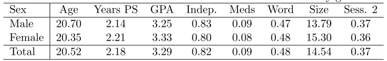
Table 2 shows that men and women were similar in terms of age, GPA, years of post secondary

schooling (Years PS) and even have the same proportion taking psychological medication (Meds).

Both genders were assigned to sessions with similar characteristics, except that on average females

were in slightly larger sessions. The session female to male ratio ranged from 0.3 to 2.3 and

averaged 1.01. Thus, all sessions had some degree of gender mix and on average this mix was about

one-to-one.

Table 2: Mean values of individual and session characteristics by gender. Sex Age Years PS GPA Indep. Meds Word Size Sess. 2 Male 20.70 2.14 3.25 0.83 0.09 0.47 13.79 0.37 Female 20.35 2.21 3.33 0.80 0.08 0.48 15.30 0.36 Total 20.52 2.18 3.29 0.82 0.09 0.48 14.54 0.37

Sessions took place three to four times a week and were held in the morning. Each session

took slightly less than an hour, including approximately 10 minutes at the beginning of the session

during which participants waited together in a foyer. This allowed participants to see that sessions

included both males and females. Once participants entered the lab, partitions were used so that

participants could not see each other’s computer screens or facial responses from the feedback

received. Competition and group memberships were also anonymous.

Payouts were based on one randomly chosen treatment, excluding the flat rate show-up payment,

payouts averaged $7.38 for the math session and $15.01 for the word sessions. Participants who

and Laury (2002). The risk aversion tasks were performed a few days after the second session to

avoid endogeneity with competition task earnings. A total of 112 participants (56 male and 56

females) participated in the risk aversion task. The average payout for the risk aversion task was

$6.57.

2.1 Task Performance

Each individual participated in five different treatments in each session. For the first three

treat-ments the compensation schemes were as follows:

Treatment 1: Piece rate ($0.50 per sum and $0.25 per word).

Treatment 2: Random sized tournament of 2, 4, or 6 individuals (the winner earned the piece rate

multiplied by the size of tournament).

Treatment 3: Group pay: an individual was paired with a randomly chosen partner and the total

production of the 2 individuals was multiplied by the piece rate and then split evenly.

Table 3: Performance Across Treatments and Gender

Math T1 T2 T3 T4 T5 Word T1 T2 T3 T4 T5 Male 10.9 12.1 12.3 12.7 12.8 Male 38.2 39.4 43.0 45.3 47.0 Female 9.9 11.4 11.8 12.3 12.1 Female 41.0 41.1 45.0 48.4 47.3 Both 10.4 11.8 12.0 12.5 12.5 Both 39.6 40.3 44.0 46.9 47.1

Table 3 shows mean performance by gender over treatments and tasks. The increasing mean

values over the first three treatments in both the math and the word tasks suggest that subjects are

learning to do the task better during the session. There are no statistically significant performance

differences between males and females in either task.8

This lack of a performance difference by

gender, for either task, removes one obvious potential reason for gender differences in choices.

2.2 Gender Differences in Competitive Choices

Niederle and Vesterlund (2007) and Gupta et al. (2005) find that when given the choice between a

tournament and piece rate females are less likely than males to enter tournaments. To test whether

this basic result can be replicated with our protocol, we focus on choices made in Treatment 4.

In those studies, individuals did not have information about their relative performance, and in

8

our study this feedback comes only after Treatment 4. The available choices of group pay, piece

rate, and tournaments of increasing size can be ordered by increasing competitiveness, with sharing

being less competitive than not sharing and larger tournaments being more competitive. In the

figures and empirical analysis we lump the two, four and six person sized tournaments together

though the results are robust when using an ordered scale for tournament size.

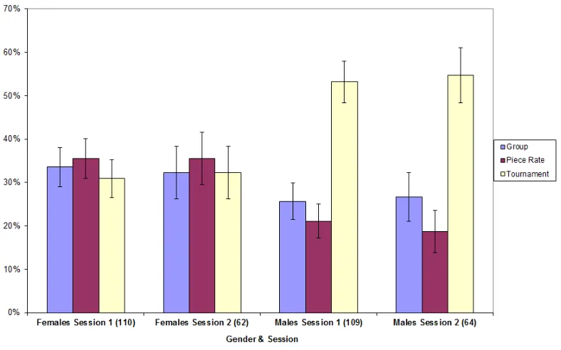
Figure 2: Choice Differences Before Feedback, by Gender and Session

Sample size in parentheses.

Figure 2 shows the distribution of choices made by males and females in the first and second

sessions for Treatment 4. The gender differences are large: pooling over sessions we find that only

31% of females chose to compete in tournaments while 54% of males chose the tournaments. The

difference persists for the piece rate: 36% of females chose the piece rate compared to only 20%

of males. These differences are all significant at the 2% level or better with chi-square tests. This

replicates earlier findings, and shows that gender differences for competitive choices are robust to

the addition of a group pay option and different sized tournaments. We also find that, on average,

males and females chose consistently across the two repeated sessions, despite the fact that these

While there are no significant differences in performance between males and females, other

factors such as age and GPA might conceivably affect compensation choices. In this design, we

predict that with full information about abilities individuals would sort according to ability, with the

least able individuals choosing the least competitive environments and the higher ability individuals

choosing more competitive tournaments. Given this we use an ordered probit to test whether the

gender differences in the probability of selections remain after controlling for other potentially

relevant factors.

Table 4 shows that the gender differences persist with these controls, along with the addition

of control variables for confidence, performance, and improvement in the repetition of tasks in a

tournament. Columns 1 to 3 use CompScale as the dependent ordinal variable, where group pay

compensation is less competitive than piece rate which is less competitive than a tournament of

any size.9

. In the results, we include both pooled results and random effects estimations using an

ordered probit model. For nonlinear estimations such as ordered probits, random effects models are

often used to deal with the difficulties and bias involved with using fixed effects models (Arellano

and Honor´e 2001). Given that the experiment data is considered a short panel, any fixed effects

estimation of a nonlinear model would also suffer from the well-known incidental parameter problem

that may bias fixed effects results (Greene 2004). For these reasons we chose to use a random effects

ordered probit for estimation purposes.

Table 4 replicates the results of Niederle and Vesterlund (2007) with Treatment 4, before

rel-ative performance feedback. Females are less likely than males to enter tournaments, even when

controlling for individual confidence (Confidence (T1)) and relative rank of performance within the

session (%-tile Rank (T1)) from the first treatment. The %-tile Rank (T1) variable gives the rank of

an individual based on her or his performance in Treatment 1 in the session. Using rank allows us to

have the same measure for both math and word tasks.10

Confidence is measured by an individual’s

predicted performance at the end of Treatment 1 (prior to finding out their actual performance)

divided by that individual’s prediction of the average performance of all session participants.11

To

control for performance, we use the relative rank from Treatment 1, but the results are unchanged

when using absolute performance along with an interaction term for word based tasks.

9

Our results are consistent with a multinomial logit model and from using ordered probits with rankings that treat larger tournaments as more competitive.

10

Using a variable that measures actual performance with an interaction term for the type of task, gives the same results as are presented here.

11

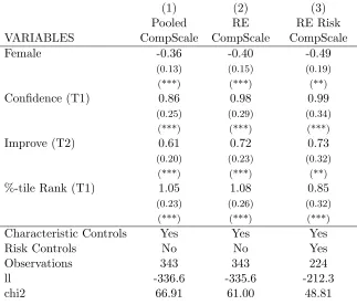
Table 4: Ordered Probit Estimates: Choices for No Relative Information Treatment

(1) (2) (3)

Pooled RE RE Risk VARIABLES CompScale CompScale CompScale

Female -0.36 -0.40 -0.49

(0.13) (0.15) (0.19) (***) (***) (**)

Confidence (T1) 0.86 0.98 0.99

(0.25) (0.29) (0.34) (***) (***) (***)

Improve (T2) 0.61 0.72 0.73

(0.20) (0.23) (0.32) (***) (***) (**)

%-tile Rank (T1) 1.05 1.08 0.85

(0.23) (0.26) (0.32) (***) (***) (***)

Characteristic Controls Yes Yes Yes

Risk Controls No No Yes

Observations 343 343 224

ll -336.6 -335.6 -212.3

chi2 66.91 61.00 48.81

Pooled means pooled cross section. RE means that random effects were used. Standard errors in parentheses. p<0.01, ** p<0.05, * p<0.10

As expected, both confidence and the actual percentile rank from the first treatment are

posi-tively correlated with the selection of more competitive environments. Improvement in performance

between the first and second task (Improve (T2)) also has a significant positive effect. These

re-gressions include controls for individual specific characteristics, including the number of years of

college, psychoactive medication, GPA, and age.12

The results are similar when using a random

effects ordered probit, in column 2. Column 3 includes a measure of risk aversion for individuals

that participated in a task similar to the one used by Holt and Laury (2003). We find that this

measure of risk aversion is not significantly correlated with competitive choices in Treatment 4.

The marginal effects (calculated from column 1) show that a female has a 0.14 lower probability

of choosing a tournament than a male, even when controlling for performance and confidence. For

a female to be as likely to choose a tournament as an average male, we would have to increase

her belief about her performance relative to the average by 40%, which is a significant increase in

overconfidence. A ten-percentile improvement in actual relative performance would increase the

12

probability of entering a tournament by 0.04. A female would have to improve her percentile rank

by 34% to be as likely to enter a tournament as a male. Thus, these gender differences are not just

significant, but they are also large.

After each treatment, before receiving any feedback, subjects were asked how many correct

answers they believed they submitted. Subjects were paid ($0.25) for each correct answer to

en-courage accurate answers. We create a measure of confidence by dividing an individual’s prediction

of how well he or she did divided by his or her prediction of the session average for that treatment.

Since the average individual should believe they did not perform any better than the session

aver-age, this confidence measure should have a mean of one – in the absence of overconfidence.13

We

could have asked for rank estimates instead of performance estimates, but rank is a poor measure

of the degree of over or under confidence. Consider two individuals that think they are ranked first

in their respective group. One may think that he is 10% better than the average while the other

may think she is 50% better. Both these individuals would be treated as having the same level

of confidence with the rank measure, but one individual is actually much more confident. We use

the measure of confidence from the first treatment because every subject performed the task for

this treatment under the same piece rate form of compensation. This confidence variable provides

the earliest measure of overconfidence before experiencing any feedback or differing experimental

manipulations.

Changes in performance as the experiment proceeds could also change confidence. The variable

Improve (T2), measured as the ratio of the individual’s performance from Treatment 2 divided by

the performance in Treatment, captures the effect of individual improvement between Treatment 1

(piece rate) and Treatment 2 (tournament). There are two possible reasons that this variable should

matter: First, individuals may feel that they improve more than the average individual or that they

were unlucky in Treatment 1 compared to how others would have performed. Second, it may be

the case that individuals become more motivated to put in greater effort because of the competitive

nature of the tournament in Treatment 2. Individuals that improve a lot from competing in such

settings would be more likely to choose to compete than individuals whose performances are not

positively affected by competitive settings.

13

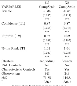
Table 5: Gender Effects (Clustered Errors)

(1) (2)

VARIABLES CompScale CompScale

Female -0.35 -0.35

(0.135) (0.114) *** ***

Confidence (T1) 0.87 0.87

(0.256) (0.246) *** ***

Improve (T2) 0.62 0.62

(0.181) (0.187) *** ***

%-tile Rank (T1) 1.04 1.04

(0.227) (0.233) *** ***

Clusters Individual Session

Risk Controls No No

Characteristic Controls Yes Yes

Observations 343 343

chi2 71.85 116.8

ll -336.5 -336.5

Robust standard errors in parentheses *** p<0.01, ** p<0.05, * p<0.1

Niederle and Vesterlund (2007) found that part of the difference between male and female

willingness to compete was driven by males being more overconfident than females. In their study,

independent of confidence, females had a 0.16 lower probability of entering a tournament than

males. Using our measure of confidence we find that the gender difference is nearly the same, 0.14.

Since we have multiple observations from the same individuals and individuals participate in

the same sessions, we also run regressions where we cluster standard errors on experiment sessions

and then also separately on individuals. Table 5 shows that the results concerning females being

less likely to enter in tournaments without relative performance feedback remain consistent when

using errors that are clustered on the specific experiment session or on the individual. In this table

the dependent variable is the same ordered variable of competitiveness used previously where group

pay is less competitive than piece rate and piece rate is less competitive than a tournament of any

size.

Our within-subjects design includes one session of math treatments and one of word treatments.

G¨unther et al. (2010) found that in a maze task, men increased performance in reaction to

attribute this to a ”stereotype threat” arising from beliefs that women are not good at the maze

task. This could logically lead to different choices by women to compete, with different tasks.

Fig-ure 3 shows that in our data there is little difference in the selection of competitive environments

by females regardless of the type of task used. We also find little difference in choices by males as

more than 50% of males chose to compete in tournaments in both math and word tasks.

Figure 3: Selection Differences for Females by Task Type for No Information Treatment

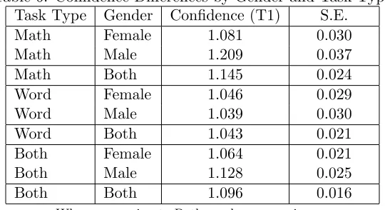
Table 6 looks at confidence differences by gender and task. Both genders are overconfident on

average. Males are significantly more overconfident in their math abilities than females, and there

is no significant difference in confidence between males and females in the word task. There is no

significant difference among females between the math and word tasks, while males are significantly

more confident in their math performance than in their word task performance. On average, males

are slightly more confident in their abilities than females. This is partly driven by a few high ability

males who are correct in believing they are better than the average, but overestimate the degree.

For example, the highest level of confidence for a male is 3.38 times his prediction of the average.

His actual performance is 2.29 times the actual session average. Overall, males and females are

than females in both math and word tasks even though male overconfidence is higher in the math

task. The type of task was not significant in regressions for choices, with or without confidence

controls.

Table 6: Confidence Differences by Gender and Task Type Task Type Gender Confidence (T1) S.E.

Math Female 1.081 0.030

Math Male 1.209 0.037

Math Both 1.145 0.024

Word Female 1.046 0.029

Word Male 1.039 0.030

Word Both 1.043 0.021

Both Female 1.064 0.021

Both Male 1.128 0.025

Both Both 1.096 0.016

When comparing to Both genders, removing an outlier makes the gender difference insignificant at a 5% level.

2.3 Performance Feedback Eliminates Gender Differences to Compete

Providing information about the quality of possible competitors might reduce mistakes in

competi-tive choices, but there is no obvious reason feedback should reduce the gender difference in choices,

if that difference is primarily driven by preferences. We test the effect of performance feedback

on choices by providing subjects with an ordered list of the performance of all the participants in

their session from Treatment 1, with their own performance highlighted, before they choose their

Treatment 5 compensation scheme. This provides information about the quality of their potential

competitors, if they choose to enter a tournament.

The two groups of bars on the left side of Figure 4 suggest that females’ choices are barely

affected by information about the performance of potential competitors. The right side of the figure

shows that males’ choices change dramatically. There is a significant increase in the proportion

of males choosing piece rate (5% significance level) and group pay (10% significance level), and

a significant decrease in the proportion choosing tournaments (5% significance level). Comparing

the distributions of men’s and women’s choices in Treatment 4 gives a Pearson chi-square statistic

of 18.79 (p-value: 0.000). After relative performance feedback in Treatment 5 male and female’s

Figure 4: Selection Differences by Gender and Information Treatment (Treatments 4 and 5)

Females (172), Males (173). Sample size in parentheses.

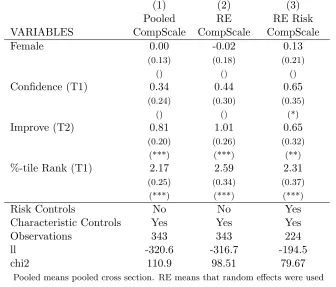
Table 7 shows the results from three different types of ordered probits for Treatment 5 choices,

using the CompScale competitiveness definition from the Treatment 4 analysis. Columns 1 through

3 show, that once performance feedback is provided, there are no significant differences between male

and female choices. Instead, we find that choices are very dependent on the relative performance

information, and on the individual’s improvement from Treatment 1 to Treatment 2. Risk aversion

control variables are not significantly correlated with compensation choices on average; though

risk aversion measures were significant when only examining high ability individuals’ choices in

Treatment 5. The one variable that consistently affects individual choices in Treatment 5 is an

individual’s percentile rank from Treatment 1, a summary statistic of the feedback information

provided before the Treatment 5 choice.

The overall conclusion from Figure 4 and the probits in Table 7 is that there are no significant

gender differences in competitive choices when subjects are fully informed of their relative

perfor-mance compared to potential competitors. In the next section we consider the costs of the selection

differences between men and women when they lack information about the quality of competitors

Table 7: Ordered Probit Estimates: Choices for Relative Information Treatment

(1) (2) (3)

Pooled RE RE Risk VARIABLES CompScale CompScale CompScale

Female 0.00 -0.02 0.13

(0.13) (0.18) (0.21)

() () ()

Confidence (T1) 0.34 0.44 0.65

(0.24) (0.30) (0.35)

() () (*)

Improve (T2) 0.81 1.01 0.65

(0.20) (0.26) (0.32) (***) (***) (**)

%-tile Rank (T1) 2.17 2.59 2.31

(0.25) (0.34) (0.37) (***) (***) (***)

Risk Controls No No Yes

Characteristic Controls Yes Yes Yes

Observations 343 343 224

ll -320.6 -316.7 -194.5

chi2 110.9 98.51 79.67

Pooled means pooled cross section. RE means that random effects were used Standard errors in parentheses

*** p<0.01, ** p<0.05, * p<0.1

2.4 The Cost of Choices and the Effect of Feedback, by Gender and Ability.

To give some sense of the costs of gender differences in choices, we simplify and assume people

maximize expected payoffs, keep effort constant across compensation choices, and take the choices

and performance of others as given. Table 8 shows the average expected value losses for the

suboptimal selections by males and females in Treatment 4 and Treatment 5.14

Each column

represents the optimal choice that should have been made. The numbers represent the average

expected value cost for choosing something other than that optimal choice. For example, in the

first row under column 6 (for the 6 person sized tournament), the 27.27 represents the average

loss to females whose optimal choice was a tournament of six, but who instead chose a different

form of compensation. The Avg Loss column provides the average loss by gender and treatment.

The average loss of 6.78 in the first row means that females lost an average of $6.78 from their

suboptimal choices in Treatment 4.

14

Table 8: Selection Losses

Average Loss from Suboptimal Decisions Optimal Choice

Treatment Gender Grp PR 2 4 6 Avg Loss

4 Female Avg Loss 1.58 2.28 2.91 6.80 27.27 6.78 4 Male Avg Loss 2.42 2.97 2.31 3.29 12.60 4.91 5 Female Avg Loss 0.88 1.88 2.21 5.93 18.70 4.80 5 Male Avg Loss 1.39 1.49 2.02 4.79 10.98 3.95

In Treatment 4, the average expected value loss from selection mistakes was $4.91 for males

and $6.78 for females, a statistically insignificant difference with a t-test. These loss differences

are mostly driven by high ability females choosing not to compete, and to a lesser extent by low

ability males choosing to compete. Column 6 shows that many high ability females (those who

should select a tournament size of 6) are instead selecting smaller tournaments or group pay or

piece rate, at a large cost. The top females lose $27.27 in expected value compared to $12.60 for the

top males. In contrast, low ability males make only slightly more costly decisions than low ability

females, averaging $2.42 versus $1.58 for the lowest types of each gender. We find that high ability

females and high ability males are not entering competitive environments enough. But the high

ability females overwhelming select the noncompetitive environments of piece rate and group pay,

which are very costly decisions. In contrast, too many low ability males are entering competitive

environments, but these mistakes are not particularly costly, on average, because low ability males

would not perform well in the piece rate either.

Table 8 also shows that relative performance feedback decreases the average expected value

losses for both males and females and shrinks the gender gap as well. The decreases in expected

value losses are greatest for high ability females, whose average expected loss fell from $27.27 in

Treatment 4 to $18.70 in Treatment 5, while losses for high ability males fell from $12.60 to $10.98.

Low ability females and males tend to move towards group pay as they get performance feedback.

While a gender difference remains, with low ability males making more expensive mistakes than

women, the cost differences are small.

In Figure 5, we turn to the question of how relative feedback information affects the choices of

high ability females and males. A high ability individual is defined as an individual who should

enter a four person tournament or larger to maximize expected returns from competition. Figure

Figure 5: Information Effects for Decisions by High Ability Types

Females (45), Males (50). Sample size in parentheses.

high ability females entering tournaments. Over 50% of high ability females enter tournaments

when given relative performance feedback, which is significantly more than the 31% that choose

tournaments before receiving the performance feedback. In testing for distributional changes, we

find that there is a significant difference in choices for females between Treatment 4 and Treatment

5; using a Pearson chi-square test the level of significance is p= 0.034.

With information, fewer high ability males enter tournaments (12% fewer), but this change in

tournament selection is not statistically significant at the 5% level. The distributional difference of

choices for high ability males coming from information feedback is not significant as a chi-square

test comparing high ability males between treatments produces a level of significance ofp= 0.317.

Without feedback in Treatment 4, there is a significant difference in the distributions of competitive

choices between males and females (p= 0.000). After receiving feedback as the level of significance

using a χ2 test is p = 0.158. Thus, relative performance feedback seems to eliminate most of the differences in choices between the high ability females and high ability males.

Figure 6 shows the effect of relative performance information on choices by low ability types,

respec-Figure 6: Information Effects for Decisions by Low Ability Types

Females (99), Males (90). Sample size in parentheses.

tive session from Treatment 1. The largest effects are for males. Information drops the percentage

of low ability males choosing tournaments from 43% to 22%, and increases the percentage of low

ability males choosing group pay from 37% to 51%. For low ability males, the difference in the

dis-tribution of competitive choices between Treatment 4 and Treatment 5 is significant at ap= 0.010

with a chi-square test. No such significant difference occurs for low ability females. The

distri-butions of choices are significantly different for low ability females and males in Treatment 4 as

chi-square test lead to ap= 0.054. But in Treatment 5 there are no significant differences between

distributions for low ability females and males.

Information about relative performance moves high ability females towards more competitive

choices and low ability males away from tournaments towards less competitive types of pay. Low

ability females show only a small movement away from group pay towards piece rate. Overall,

2.5 Competitiveness Differs Between High and Low Hormone Phases of

Men-strual Cycle

Normal cycling women experience large changes in hormone levels across the menstrual cycle (Figure

1) and these variations are similar in women using hormonal contraceptives. As explained in the

design section, we used a screening survey to schedule females for one session during a low-hormone

phase and one during a high-hormone phase and exit surveys to confirm phases.

Table 9: Menstrual Cycle Regularity Regularity of Period Percent Count

Identical 14.3% 55

Within 1-2 days 42.3% 163

Within 3-7 days 34.3% 132

Very Irregular (7+) 9.1% 35

Total 385

Missed Period in Last 3 Months Percent Count

Yes 14.7% 57

No 85.3% 330

Total 387

Numbers may not add up due to item non-response in screening survey.

Table 9 summarizes the screening survey responses of females. Of the females who completed the

screening survey almost 15% missed a menstrual period during the previous 3 months. Over 43% of

these females experienced menstrual cycle irregularity of 3 days or more, suggesting that predicted

menstrual periods may have significant measurement error. Due to the potential inaccuracies

introduced by this prospective survey, we also used an exit survey with both retrospective and

prospective questions on menstruation to classify hormonal phases for our analysis.15

The screening survey also provided information on the proportion of females that use hormonal

contraceptives. Over 54% of females in our sample used some form of hormonal contraceptive in

the form of the pill or ring. This makes for easier predictability of low and high phases for these

females, since hormonal fluctuations are exogenously determined by hormonal contraceptive use.

To help identify hormonal phases for females using a hormonal contraceptive, we asked all female

participants for the start day of their hormonal contraceptive regimen.

15

Of the females that participated in experiment sessions, 62.7% of those attending a first session

were following a hormonal contraceptive regimen, as were 62.9% of those at second sessions. The

American College Health Association found that about 72% of sexually active females were using

some form of hormonal contraceptive in 2008 . In examining contraceptive use by females in the

United States, it was found that for women between the ages of 15 to 44, over 82% had at one

time taken oral hormonal contraceptives (Mosher et al. 2004), suggesting that our sample is not

unusual in terms of contraceptive use.

We hypothesize that the low-hormone phase, whether induced through endogenous or exogenous

means, is associated with similar behavioral changes for both hormonal contraceptive users and

normal cycling females. We tested this by controlling for hormonal contraceptive use and found

no systematic significant difference in behavior between hormonal contraceptive users and normal

cycling females. We therefore pool both groups of females and focus on similar differences across

the two hormonal phases.

Figure 7: Competitive Choice by Gender and Hormonal Phase

Figure 7 shows the distribution of competitive choices of females by phase, along with choices

in the two phases. They are more than twice as likely to choose group pay when they are in the

low phase, and twice as likely to choose tournament when they are in the high phase, though still

not as likely as men. When we include controls in regressions, this last difference will become

insignificant. The data for the histogram includes all females and males that attended two sessions

and all females who could be identified as being in the low or the high phase. Due to the difficulty

of predicting the low phase, some females were identified by the exit survey as being in the same

phase for both word and math tasks. As well, some phases could not be accurately identified and

those subjects are not included in the analyses.

These differences in competitive environment choices across hormonal phases may result from

differences in expected performance changes across the menstrual cycle, or from different preferences

for competition. We find that for the most part, there are no significant performance differences

between females in the low phase and those that are not in the low phase.16

It is also possible

that females in a specific hormonal phase might experience greater aversion to certain types of

tasks; therefore, we separate out these results by math and word tasks. Figure 8 shows female

compensation choices before feedback by hormonal phase and task type. Females that participated

in a math or word task during the low phase were then scheduled for the other type of task when

in a high phase, and vice-versa. The figure shows that the general correlation between competitive

choice and menstrual phase holds across tasks: high phase females are less likely to choose group

pay and more likely to choose tournaments in both word and math tasks.

We use ordered probits to examine the statistical significance of gender and menstrual phase

before feedback, while including control variables. Table 10 uses the CompScale variable, an ordered

categorical variable with choices ranked from group pay, piece rate, to tournament. The first column

provides pooled cross-sectional results including all subjects, the second to fourth columns provide

estimates using random effects ordered probit. The second column includes all males and females,

the third column consists of a female only sample and the fourth column takes into account only

males and females for which risk aversion measures were available.17

We find that females in the low phase select noticeably less competitive compensation plans than

females in the high-hormone phase. In fact much of the average difference in competitive choices

between males and females is driven by the choices of the low phase females. This result holds

even when controlling for confidence. It is worth noting that there are no significant differences in

16

See Appendix B.1

17

Figure 8: Compensation Choice by Hormonal Phase and Task Type for Females.

We are comparing females that attended two sessions. Sample size in parentheses.

confidence levels between low hormonal phase and high hormonal phase females, and yet females

in the low phase avoid the competitive environments of tournaments and are more likely to choose

the least competitive setting possible, group pay.

These differences could potentially result from discomfort during the low-hormone phase of

menstruation. But females in the low-hormone phase do not behave differently from any other

group once they receive relative performance feedback. Thus, physical discomfort is an unlikely

explanation for these systematic differences in low information settings.

The magnitudes of the marginal effects (calculated using the pooled cross sectional estimates)

of being in the low-hormone phase are substantial and are larger than the average gender effects.

For group pay, females on average have a 0.08 higher probability of choosing group pay than males.

Females in the low phase have an additional 0.16 higher probability of choosing group pay. For

tournaments, females have a 0.10 lower probability of choosing a tournament when compared to

males, and females in the low-hormone phase have an additional 0.16 decrease in the probability

Table 10: Ordered Probit: Hormone Effects for No Relative Information (Treatment 4)

(1) (2) (3) (4)

Sample All All Females Only Risk

VARIABLES Pooled RE RE RE

Female -0.26 -0.29 -0.26

(0.14) (0.16) (0.21)

(*) (*) ()

Low Phase -0.44 -0.46 -0.53 -0.76

(0.21) (0.22) (0.26) (0.27) (**) (**) (**) (***)

Confidence (T1) 0.81 0.91 1.08 0.90

(0.26) (0.30) (0.54) (0.35) (***) (***) (**) (**)

Improve (T2) 0.60 0.69 0.79 0.72

(0.20) (0.23) (0.38) (0.32) (***) (***) (**) (**)

%-tile Rank (T1) 0.97 0.99 0.52 0.72

(0.23) (0.26) (0.43) (0.32) (***) (***) () (**)

Risk Controls No No No Yes

Characteristic Controls Yes Yes Yes Yes

Observations 328 328 155 211

ll -322.3 -321.7 -156.0 -197.4

chi2 64.32 58.60 19.76 51.31

Dependent variable is CompScale where -1 is group pay, 0 is piece rate, and 1 is a tournament. The total low phase females that could be identified for data analysis is 45.

Pooled means pooled cross section. RE means that random effects were used. Standard errors in parentheses

*** p<0.01, ** p<0.05, * p<0.1

The changes over the menstrual cycle are also large relative to the effects of confidence and

performance. For a female in the low phase to have the same probability of entering a tournament

as a female in the high phase we would have to increase her belief about her performance relative

to the average by 50%. In terms of an equivalent performance effect, a female in the low-hormone

phase would have to improve her percentile rank by 42% to be as likely to enter a tournament as

a female in the high-hormone phase.

Table 11 shows that the results concerning females in the low hormonal phase persist when

using standard errors that are clustered on the specific experiment session or on the individual for

the no information treatment. In this table the dependent variable is the same ordered variable

of competitiveness that was used previously. The results are entirely consistent with our previous

Table 11: Hormone Effects (Clustered Errors) (1) (2) SE Clusters Individual Session

Female -0.25 -0.25

(0.149) (0.137)

* *

Low Phase -0.45 -0.45

(0.200) (0.156) ** ***

Confidence (T1) 0.84 0.84

(0.275) (0.234) *** ***

Improve (T2) 0.62 0.62 (0.182) (0.187)

*** ***

%-tile Rank (T1) 0.96 0.96

(0.225) (0.227) *** ***

Clusters Individual Session

Risk Controls No No

Characteristic Controls Yes Yes

Observations 328 328

chi2 69.61 124.6

ll -322.2 -322.2

N clust 215 26

Robust standard errors in parentheses *** p<0.01, ** p<0.05, * p<0.1

in mixed gender settings, it seems that hormonal phase may be a driving factor that needs to be

considered in low information settings.

Interestingly, relative performance feedback makes these cycle specific effects disappear. Table

12 provides the results from ordered probit estimations for Treatment 5, where subjects were

pro-vided with relative performance information from Treatment 1 prior to making their competitive

environment selections. Table 12 shows that when participants are informed of their relative

perfor-mance compared to other potential competitors, then there is little difference in selection between

genders or across the menstrual cycle.

As with the gender differences, we find that after participants are informed of the quality of

potential competitors, choice differences across the menstrual cycle become insignificant. We find

that choices after feedback mainly depend on the relative performance information provided prior

to Treatment 2. Though females’ choices to avoid competitive environments are most frequent in

the low-hormone phase, these results suggest that this effect seems to be linked with the information

available about the quality of potential competitors.

Table 12: Ordered Probit: Hormone Effects after Feedback (Treatment 5)

(1) (2) (3) (4)

Sample All All Females Only Risk

VARIABLES Pooled RE RE RE

Female -0.07 -0.13 0.10

(0.15) (0.20) (0.24)

() () ()

Low Phase 0.03 0.13 0.12 -0.12

(0.21) (0.25) (0.27) (0.29)

() () () ()

Confidence (T1) 0.23 0.32 0.21 0.54

(0.25) (0.31) (0.53) (0.36)

() () () ()

Improve (T2) 0.76 0.92 1.06 0.49

(0.20) (0.26) (0.40) (0.33) (***) (***) (***) ()

%-tile Rank (T1) 2.18 2.61 2.63 2.33

(0.25) (0.35) (0.55) (0.38) (***) (***) (***) (***)

Risk Controls No No No Yes

Characteristic Controls Yes Yes Yes Yes

Observations 328 328 155 211

ll -307.8 -303.9 -143.3 -183.4

chi2 104.7 93.82 45.89 75.79

We identified 45 females as low phase for this analysis. Pooled is pooled cross section, RE is random effects.

Standard errors in parentheses *** p<_{0.01, ** p}<_{0.05, * p}<_0.1

As discussed previously, there is a cost associated with high ability individuals avoiding

compet-itive settings, and with low ability individuals choosing tournaments. We find that females in the

low-hormone phase make more costly mistakes than high phase females, and males. The average

expected value losses for males, low phase and high phase females in Treatment 4 are shown in

Ta-ble 13. Low phase females sacrifice the greatest amount of expected value from making suboptimal

choices, $8.50. The expected value losses for high phase females and males are $6.52 and $4.91.

The differences between low and high phase females and between males and high phase females are

not statistically significant, but low phase females make more costly choices than males at the 5%

Table 13: Expected Value Loss in Treatment 4 Mean Std. Error

Male 4.91 0.72

Female Non-Low 6.52 1.30 Female Low 8.50 2.57

These results show that menstrual phase and the corresponding hormone levels are correlated

with competitive choices, but only if the strength of the competition is not known. If there is

little information about the relative abilities, then females in the low-hormone phase make more

costly decisions than males and non-low phase females. But there are no significant differences in

expected value losses between genders or between different hormonal phases for females if good

relative performance information is available.

2.6 Systematic Absenteeism, Cancellations, and Tardiness

Absenteeism, cancellations, and tardiness are frequent in experiments, but their effect on sample

composition and results are poorly understood. In this study, because of the screening and exit

surveys, we know some of the characteristics of those who missed a scheduled session, canceled

at the last moment, or showed up late. Our recruiting procedures were designed to ensure we

would observe females during both the high phase and the shorter low-hormone phase. Due to

the variation of the menstrual cycle, it is difficult to predict the low hormonal phase for females.

Using the screening survey, female subjects were scheduled for their sessions according to their

predicted cycle day, calculated using self reported data about the start of previous menstrual

periods. Whenever possible these data were combined with self reported data concerning females’

hormonal contraceptive regimens. Once the cycle day could be predicted, then a set of possible

session days were provided to potential participants and they chose and confirmed a day with a

research assistant. For individuals to be considered as scheduled, they had to confirm that they

would attend a specific session.

Table 14 shows the proportion of participants that attended the experiment sessions as

sched-uled, meaning they were present and punctual. Females are noticeably less likely to show up than

males: 79% of the males showed up as scheduled compared to 68% of females. Based on predicted

phases, only 62% of low phase females attended as scheduled, while high phase females attended