Comparative Study on Various Random Walk
Techniques for Left Ventricle Cavity Segmentation
Ghada Abdel-Aziz
Computer science and Engineering Dept., Faculty of
Electronic Engineering, Menoufia University, Egypt
Hamdy M. Kelash
Computer science and Engineering Dept., Faculty of
Electronic Engineering,Menoufia
University, Egypt
Osama S. Faragallah
Computer science and Engineering Dept., Faculty of
Electronic Engineering, Menoufia University, Egypt
ABSTRACT
Objective of image segmentation is to group regions with coherent characteristics. This paper presents a comparative study on Random walk techniques for Left ventricle segmentation. In this paper, LV cavity segmentation is demonstrated for each technique using multi-slice MR cardiac images. The quality of segmentation process is measured by comparing the resulted images of different Random walk techniques using DICE coefficient, PSNR and Hausdorff distance. The comparison includes measuring the execution time of each technique.
General Terms
Image segmentation, Random walk techniques, LV cavity segmentation
Keywords
Image segmentation, Random walks, LV cavity extraction, segmentation techniques
1.
INTRODUCTION
The problem of localizing regions of an image relative to its content is known as image segmentation [1]. Cardiovascular Disease (CVD) is defined as any disorder in the function of the heart and circulatory system. CVD may cause death. In the fact, CVD is the main cause of death worldwide. Millions of deaths occur every year due to CVDs in high income countries like in Europe as well as in middle and low income countries. Nearly half of all deaths in Europe are from CVDs; 52% of deaths in women and 42% of deaths in men. About 85% of overall mortality of middle- and low-income countries is due to CVDs. It is expected that the number of mortality due to CVDs will increase in the next 15 years and it may reach 23.3 millions. CVDs are projected to remain the single leading cause of death [2, 3].
[image:1.595.337.533.218.428.2]The Left Ventricle (LV) is the main cavity of the heart. Most of the CVDs cause changes in the left ventricular shape. Temporal changes in left ventricular (LV) shape over the cardiac cycle provide fundamental information regarding systolic and diastolic function of the heart. The LV function analysis requires the accurate description or segmentation of ventricular shape. The segmentation process divides an image into homogeneous regions considering one or more similar characteristics [4, 5]. The manual segmentation and analysis for 3D cardiac MR images are difficult because of the increasing resolution and it is extremely time-consuming. In order to further aid the cardiologist in the segmentation process for the extraction of LV cavity, accurately and fast semi-automated segmentation methods are needed. The goal of the semi-automation of segmentation is to shorten the time and improve the reliability of the process [6].
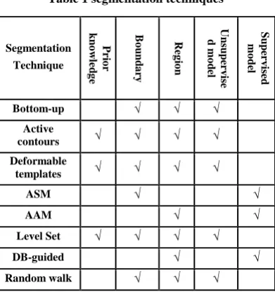
Table 1 segmentation techniques
Segmentation
Technique
Pr
io
r
k
n
o
w
le
d
g
e
B
o
u
n
d
a
ry
R
eg
io
n
U
n
su
p
er
v
ise
d
mo
d
el
S
u
p
er
v
ised
mo
d
el
Bottom-up √ √ √
Active
contours √ √ √ √
Deformable
templates √ √ √ √
ASM √ √
AAM √ √
Level Set √ √ √ √
DB-guided √ √
Random walk √ √ √
From the full scope of segmentation methods in the medical analysis, semi-automatic techniques can be divided into three major levels [7, 8]. At the first level, sequential points are predetermined by the user on or near the boundary, the boundary is found between these points using a minimal path method [9, 10]. At the second level, the algorithms require the specification of an initial boundary, then by minimizing a cost function of shape priors and image information the final segmentation can be obtained [11, 12]. At the third level, the algorithms require predetermined marked nodes, or seeds within specific regions [1, 13].
From general view of different segmentation methods, Random walk techniques are considered to be the main concern of research in this paper. Comparison between general characteristics of LV segmentation methods is shown in Table 1 [1, 14].
Basic Random walk (BRW) image segmentation which is known as Random walk with seeds was first presented in a general form by Leo Grady. Basic Random walk is a multi-label image segmentation method. It can be used for medical applications. It is based on Graph-Theoretic Electrical Potentials [6, 1].
2.
BASIC RANDOM WALK (BRW)
In basic random walker algorithm, the image is considered as a purely discrete object. It is a graph with a fixed number of vertices and edges. Each edge is assigned a real valued weight which is calculated using the weighting function [15].Basic Random walker algorithm uses user-defined marked nodes as seeds to indicate the regions of the image. Each seed specifies a location with a user-defined label. The algorithm can give labels to an unmarked pixel using the calculation of the probability that random walker starting at this unmarked node first reaches each of the seed points. The probability that a random walker starting at pixel first reaches a seed with specific user predefined marked label, can be calculated by solving the circuit theory problem that is corresponding to a combinatorial Dirichlet problem. All seed points belonging to labels other than the specific label are grounded and this specific label node is considered to be with a unit potential. The electric potentials at each unmarked node provide the probabilities. Harmonic function solves the Dirichlet problem for a given set of boundary conditions. The established connections between random walk and graph-theoretic electrical potentials are used to get convenient method to calculate the values of these probabilities. Sparse, symmetric positive-definite system of linear equations is required to be solved. Final segmentation may be derived by using the highest probability for each pixel. [13-16].
Basic Random walk algorithm can detect weak boundaries. This algorithm is formulated in discrete space (graph) using combinatorial analogues of standard operators and principles from continuous potential theory [1, 8].
2.1
Edge Weights
A graph G = V, E with vertices ʋ ∈ V, edges e ∈ E , E ⊆ V × V. An edge e , spanning two vertices, ʋiand ʋj, is denoted by eij. A weighted graph assigns a value to each edge called a weight. The weight of an edge eij, is denoted by w( eij) or wij. The degree of a vertex is di= w eij for all edges eij incident on ʋi. wij > 0 [17].
Weighting function plays an important role for a successful segmentation in the approach. Gaussian weighting function that represents a change in image intensities in the edge weights is used [18].
), ) ( exp( 2 j i
ij I I
w
1Where 𝐼𝑖 indicates the image intensity at pixel 𝑖. The value of β is a free parameter in this algorithm [1]. Performance of the weighting method depends on the selection of the free parameter β, which is decided manually. The accuracy of the output significantly depends on this parameter [19].
2.2
Combinatorial Dirichlet Problem
The combinatorial Dirichlet problem has the same solution as the desired random walker probabilities. The Dirichlet integral may be defined as:, 2
1 ]
[
2 d
D 2
For a field µ and region Ω
A harmonic function is a function that satisfies the Laplace equation:
0
2
3
Dirichlet problem is defined as the problem of finding a harmonic function subject to its boundary values. The harmonic function that satisfies the boundary conditions minimizes the Dirichlet integral since the Laplace equation is the Euler-Lagrange equation for the Dirichlet integral [1, 13].
2.3
Build the Combinatorial Laplacian
Matrix
The combinatorial Laplacian matrix as:
, 0 , otherwise nodes adjacent are v and v if w j i if d
L ij i j
i
ij 4
Where 𝐿𝑖𝑗is indexed by vertices 𝑣𝑖 and 𝑣𝑗 [16].
2.4
Partition of the Laplacian matrix
Partition the vertices into two sets, 𝑉𝑀(marked/seed nodes) and 𝑉𝑈 (unmarked/unseeded nodes) such that 𝑉𝑀 𝑉𝑈=𝑉and 𝑉𝑀∩ 𝑉𝑈= ∅ . While 𝑉𝑀 contains all seed points, regardless of their labels [14, 16].
The nodes in 𝐿 and 𝑥 are ordered such that marked nodes are first and unmarked nodes are second. When seeds are given, divide 𝐿 , 𝑥 into:
𝐿 = 𝐿𝑀 𝐵 𝐵𝑇 𝐿
𝑈
5
x = 𝑥𝑥𝑀
𝑈 6
Where 𝑥M and 𝑥U are corresponding to the potentials of the marked and unmarked nodes, respectively. The reordering and block decomposition of 𝐿 is important to describe the problem in a linear algebra framework and for applying the Dirichlet boundary conditions to the problem [20].
2.5
Finding and Solving the Linear
System
The composition of 𝐷[𝑥𝑈]:
𝐷 𝑥𝑈 =
1 2 𝑥𝑀
𝑇 𝑥
𝑈𝑇
𝐿𝑀 𝐵
𝐵𝑇 𝐿 𝑈
𝑥𝑀
𝑥𝑈
=1 2[𝑥𝑀
𝑇𝐿
𝑀𝑥𝑀+ 2𝑥𝑈𝑇𝐵𝑇𝑥𝑀+ 𝑥𝑈𝑇𝐿𝑈𝑥𝑈]
7
Differentiating 𝐷[𝑥𝑈] with respect to xU and finding the critical point [1]:
3.
HIGH SPEED RANDOM WALK
(HSRW)
Random walk with pre-computations is a fast approximate random walk method. The objective of this technique is to shift the burden of computations of an interactive algorithm to an offline procedure. This offline mode may be performed before any user interaction has taken place. In many cases, the offline mode can be very important especially in medical segmentation such as left ventricle cavity segmentation because there is substantial time between the acquisition and segmentation of the image. Medical images often exist for days or weeks on a data server before a user interacts with the image. Eigenvectors of the graph Laplacian matrix are used to approximate the Random Walker solution. It is unknown where the user will choose to place seeds so; Pre-computation phase or offline mode procedure is very difficult. Pre-computing a small number of eigenvectors of the graph Laplacian matrix is sufficient to allow for a good and in fast approximation of the solution to the interactive Random Walker image segmentation algorithm, regardless of where the seeds are placed [21, 22]. In this paper, Random walk with pre-computations method will be referred as High Speed Random Walk technique (HSRW).
From [21], computations can be performed before seeds or marked nodes are defined (offline), calculating eigenvalue / eigenvector pairs can be performed offline to find the high speed solution of eq. 8.
The eigenvalue decomposition of L is:
𝐿 = 𝑄𝛬𝑄𝑇 9
Where:
Λ is a diagonal matrix of the Laplacian k smallest eigenvalues of L.
Q is a matrix whose columns are the k corresponding eigenvectors.
By increasing k the solution will be close to the exact solution.
𝑓 is defined by:
𝐿𝑥 = 𝑓 10
Decomposition of 𝑓 corresponding to marked / unmarked nodes:
𝑓 = 𝑓𝑀 𝑓𝑈
11
By performing an eigenvector decomposition of 𝐿 from eq.9 in eq. 10:
𝑄𝛬𝑄𝑇𝑥 = 𝑓 12
𝐸 is the pseudo inverse of 𝐿.
𝐸 = 𝑄𝛬−1𝑄𝑇 13
Decompose the 𝐸, in corresponding to marked and unmarked nodes:
𝐸 = 𝐸𝑀 𝑅 𝑅𝑇 𝐸
𝑈
14
𝑅𝑇= 𝑄
𝑈𝛬−1𝑄𝑀𝑇 15
When, ɡ is eigenvector of 𝐿 with corresponding to the zero eigenvalue and it is a constant vector since 𝐿’s column sum is 0.
Decompose the 𝑔 in corresponding to marked and unmarked nodes:
𝑔 = 𝑔𝑔𝑀
𝑈
16
𝐸𝐿 = 𝐼 − 𝑔𝑔𝑇 17
From eq. 10, 13, 17, Approximate 𝑥 using 𝐸 :
𝐸𝐿𝑥 = 𝐼 − 𝑔𝑔𝑇 𝑥 = 𝐸𝑓 = 𝑄𝛬−1𝑄𝑇𝑓 18 When 𝑓𝑈= 0 calculating 𝑓𝑀 as follows:
𝐿𝑀𝑥𝑀+ 𝐵𝑥𝑈= 𝑓𝑀 19 Substitution of eq. 6, 7 in eq. 10, 18, gives:
−𝑔𝑈𝑔𝑀𝑇𝑥𝑀+ 𝑥𝑈− 𝑔𝑈𝑔𝑈𝑇𝑥𝑈= 𝑅𝑇𝑓𝑀 20 Multiply 𝐵 by eq. 20, and then subtract it from eq. 19:
𝐿𝑀+ 𝐵𝑔𝑈𝑔𝑀𝑇 𝑥𝑀+ 𝐵𝑔𝑈𝑔𝑈𝑇𝑥𝑈= 𝐼 − 𝐵𝑅𝑇 𝑓𝑀 21
when 𝐵𝑔𝑈𝑔𝑀𝑇 is a very small amount and ≈ 0
let 𝛼 = 𝑔𝑈𝑇𝑥𝑈, 𝑃 = 𝐼 − 𝐵𝑅𝑇
Then:
𝐿𝑀𝑥𝑀+ 𝐵𝑔𝑈𝛼 = 𝑃𝑓𝑀 22
𝑙𝑒𝑡 𝑓𝑀= 𝑓 + 𝑓𝑀 𝛼𝑀 23 From 23, 22 can be divided into:
𝑃𝑓 = 𝐿𝑀 𝑀𝑥𝑀 24
𝑃𝑓 = 𝐵𝑔𝑀 𝑈 25
Note that by definition of ɡ and from eq. 10:
𝑔𝑇𝑓 = 𝑔𝑇𝐿𝑥 = 0 26
𝑔𝑇𝑓 = 𝑔 𝑀𝑇 𝑔𝑈𝑇
𝑓𝑀
𝑓𝑈
27
𝑔𝑀𝑇𝑓𝑀= −𝑔𝑈𝑇𝑓𝑈= 0 28
𝑔𝑀𝑇[𝑓 + 𝑓𝑀 𝛼] = 0𝑀 29 Then, find α,
𝛼 = −𝑔𝑀
𝑇𝑓 𝑀
𝑔𝑀𝑇𝑓 𝑀
,
30
From eq. 20,
𝑥𝑈= 𝑅𝑇𝑓𝑀+ 𝑔𝑈𝛼 + 𝑔𝑈𝑔𝑀𝑇𝑥𝑀 31
𝑥𝑈 ≈ 𝑅𝑇𝑓𝑀+ 𝑔𝑈𝛼 32
4.
EXTENDED RANDOM WALK
(ERW)
relationships in consideration. On the other hand, the objects of interest may be reasonably characterized by the intensity distribution. Random walk segmentation algorithm (BRW) is a multi label image segmentation method that can especially be used with medical images. It performs well on a wide variety of images but this algorithm has properties that could be problematic for certain segmentation tasks. Each segment must be connected to a seed and only intensity gradients were used instead of employing absolute intensity information. The goal of the extended random walker (ERW) is to combine the intensity profiling and long-range aspects of the density estimation approach with the spatial cohesion of the random walker. ERW uses an intensity model obtained via density estimation so that it could be able to integrate intensity information into the random walk spatial algorithm [6, 23].
ERW method is an extended method from the basic random walk BRW approach by employing image priors. Each seed node is connected to every other node with weight corresponding to the prior density of the pixel intensity to that label,
𝑤𝑖𝑗 = 𝑒𝑥𝑝 −𝛽 𝐼𝑖− 𝐼𝑗 2
A set of real-valued priors 𝜆𝑖𝑠, that represent the probability density that the intensity at node vi and belong to the intensity distribution of label 𝑔s
𝑥𝑖𝑠 = 𝜆𝑖𝑠
𝜆𝑖𝑞
𝑘 𝑞=1
33 This equation in vector notation may be written as,
𝛬𝑞 𝑘
𝑞=1
𝑥𝑠 = 𝜆𝑠 34
Where 𝛬𝑠 is a diagonal matrix with the values of 𝜆𝑠 on the diagonal.
λ is a vector of the prior probabilities for each node, weighted by a scalar, γ. The Laplacian is augmented with auxiliary nodes.
The Laplacian matrix is divided into components corresponding to the marked, unmarked, and auxiliary nodes:
𝐿 =
𝐿𝑀 𝐵 0
𝐵𝑇 𝐿
𝑈+ 𝛾𝐼𝑈 −𝛾𝜆
0 −𝛾𝜆 𝛾𝐼𝑈
35
Using the same way as eq. 8,
𝐿𝑈+ 𝛾𝐼𝑈 𝑥𝑈= −𝐵𝑇𝑥𝑀+ 𝛾𝜆 36
5.
EXPERIMENTAL RESULTS
The proposed methods are implemented in MATLAB with processor 2.27 GHz Intel ® core ™ i3 CPU and 3 GB memory. The seeds are defined by the user. Where K = 80 and β=30.
Similarity is computed between the result image of the algorithms and the manual segmented image as a reference.
DICE =2(A ∩ B) A + B
Where A, B are the reference mask region and the result mask region of an algorithm.
PSNR = 10 log10
d MSE(A, B)
Where d is the maximum possible value of the image and
MSE A, B is the mean square error computed between A and B.
MSE A, B = 1
MN A m, n − B(m, n)
2 N
n=1 M
m=1
Hausdorff = max(D A, B , D B, A )
Where A, B are the reference contour and the result contour of an algorithm.
D A, B = maxx∈A(miny∈B( x − y ))
Multi-slice MRI cardiac images are used. All images were stored in the standard digital imaging and communications in medicine (DICOM) format [24].
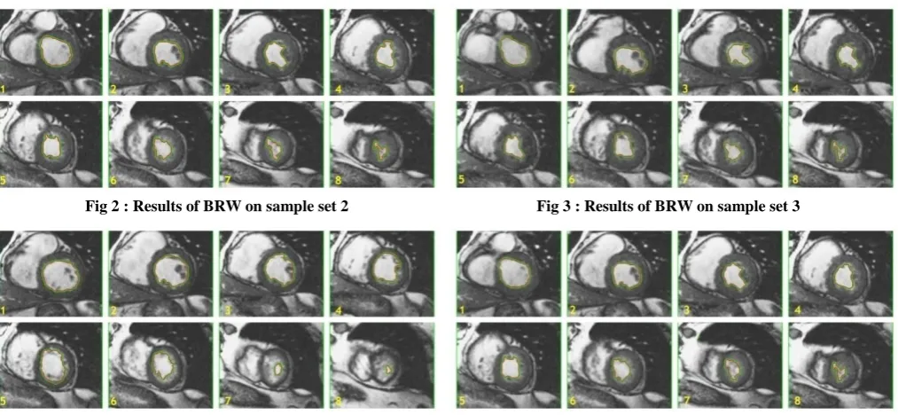
Figure 1, figure 2 and figure 3 show the resulted images of Basic Random Walk segmentation on a sample sets. High speed random walk technique is applied on the same sample sets as shown in figure 4, figure 5 and figure 6. Figure 7, figure 8 and figure 9 demonstrate the high quality segmentation using Extended random walk on the same sample sets where γ=0.0001.
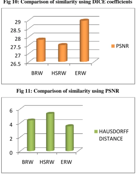
Experimental results show that basic random walk algorithm can perform LV segmentation process of good quality and its similarity may reach values over 97% in average time of 0.85 seconds per slice.
HSRW algorithm results have very close similarity values as BRW but with a little bit lower quality and much more execution speed. The pre-computations in the offline mode reduce the execution online time. The average execution time of HSRW is 0.09 seconds per slice. When K=80. Increasing the value of K will increase the similarity and make the segmentation more accurate but it will also reduce the execution speed.
The results of ERW segmentation method show that this technique has the best quality segmentation. Similarity may exceed 98%. The average execution time is about 0.86 seconds per slice.
The average of quality measurements of segmentation are calculated and recorded in Table 2, Table 3 and Table 4 for each technique.
Table 2 : Comparison of similarity using DICE coefficients
SEGMENTATION
TECHNIQUE DICE
BRW 0.966721
HSRW 0.964817
ERW 0.972700
Table 3 Comparison using PSNR
SEGMENTATION
TECHNIQUE PSNR
BRW 27.82928
HSRW 27.49958
[image:5.595.51.563.77.735.2]ERW 28.96782
Table 4 : Comparison using Hausdorff distance
SEGMENTATION TECHNIQUE
HAUSDORFF DISTANCE
BRW 4.363283
HSRW 5.309596
ERW 3.542988
Table 5 : Comparison of speed using the average of Execution time
SEGMENTATION
TECHNIQUE EXECUTION TIME
BRW 0.848492
HSRW 0.090574
ERW 0.858959
[image:5.595.47.554.514.748.2]Fig 1: Results of Basic Random Walk on sample set 1
Fig 2 : Results of BRW on sample set 2 Fig 3 : Results of BRW on sample set 3
Fig 6 : Results of HSRW on sample set 3 Fig 7 : Results of ERW on sample set 1
[image:6.595.50.551.71.490.2]Fig 8 : Results of ERW on sample set 2 Fig 9 : Results of ERW on sample set 3
Fig 10: Comparison of similarity using DICE coefficients
Fig 11: Comparison of similarity using PSNR
Fig 12 : Comparison of similarity using Hausdorff distance
Fig 13 : Comparison of Execution running time in seconds
6.
CONCLUSION
In this paper, a comparative study has been carried out on three main Random walk techniques. Each technique is applied to extract the left ventricle cavity of the heart. The comparison is done by measuring the quality of segmentation using DICE coefficient, PSNR and Hausdorff distance. The execution time is measured for each technique.
Basic Random walker technique uses user-defined marked nodes to indicate regions of the image. The algorithm can give labels to an unmarked node using the calculation of the probability that random walker starting at this location first reaches each of the user defined points.
High speed random walk technique is a fast approximate random walk method. An offline procedure that may be performed before the user interaction has taken place. Eigenvectors of the graph Laplacian matrix are calculated to get the approximate random walk solution.
Extended random walk technique uses an intensity model obtained via density estimation in order to integrate intensity information into the random walk spatial algorithm. The objects of interest may be reasonably characterized by the intensity distribution of the image.
The Experimental results show that Extended random walk technique is the one of the highest quality results compared to 0.96
0.965 0.97 0.975
BRW HSRW ERW
DICE
26.5 27 27.5 28 28.5 29
BRW HSRW ERW
PSNR
0 2 4 6
BRW HSRW ERW
HAUSDORFF DISTANCE
0 0.2 0.4 0.6 0.8 1
BRW HSRW ERW
[image:6.595.53.283.459.752.2]the other random walk techniques. Indeed, Extended random walk technique is the most accurate when it comes to similarity measurements with the corresponding manual segmentation results. The results show that the DICE coefficient of the extended random walk could reach over 98%. In High speed random walk technique, similarity results are close to the corresponding similarity measurements of the Basic random walk technique. High speed random walk results are of a little bit lower quality and much more execution speed than the basic random walk technique. The pre-computations of High speed random walk in the offline mode reduce the execution online running time.
Future work may include further studies on other different characteristics of each random walk technique. Also, two or more of the random walk techniques characteristics and features may be mixed together in order to improve the reliability of the left ventricle cavity segmentation process in order to make new hybrid random walk technique that could have the advantages such as accuracy and speed of execution to be enhanced and exclude the different disadvantages of each technique.
7.
REFERENCES
[1] L. Grady, “Random Walks for Image Segmentation” IEEE Transactions On Pattern Analysis and Machine Intelligence, vol. 28, no. 11, pp. 1768–1783, November 2006.
[2] Nichols M, Townsend N, Luengo-Fernandez R, Leal J, Gray A, Scarborough P and Rayner M. "European Cardiovascular Disease Statistics 2012". European Heart Network, Brussels, European Society of Cardiology, Sophia Antipolis, 2012.
[3] http://www.who.int/mediacentre/factsheets/fs317/en/inde x.html
[4] K. S. Fu and J. K. Mui, "A survey on image segmentation," Pattern Recognition, vol. 13, no. 1, pp. 3-16, 1981.
[5] R. Duda, P. Hart and D. Stork, "Pattern Classification", New York: Wiley-Interscience, 2000.
[6] L. Grady and G. Funka-Lea, "Multi-Label Image Segmentation for Medical Applications Based on Graph-Theoretic Electrical Potentials", Proc. Workshop Computer Vision and Math. Methods in Medical and Biomedical Image Analysis, pp. 230-245, May 2004. [7] S. D. Olabarriaga and A. W. M. Smeulders, "Interaction
in the segmentation of medical images": A survey. Medical Image Analysis, 5(2):127–142, 2001.
[8] Y. Kang, K. Engelke, and W. A. Kalender. "Interactive 3D editing tools for image segmentation". Medical Image Analysis, 8(1):35–46, 2004.
[9] L. Cohen and R. Kimmel, "Global minimum for active contour models: A minimal path approach", International Journal of Computer Vision, 24:57–78, 1997.
[10] W. Barrett and E. Mortensen, "Interactive live-wire boundary extraction". Medical Image Analysis, 1:331– 341, 1997.
[11]M. Kass, A.Witkin, and D. Terzopoulos, "Snakes: Active contour models", Int’l J on Computer Vision, 1(4):321– 331, 1987.
[12]T. F. Chan and L. A. Vese, "Active contours without edges". IEEE Trans. on Image Processing, 10(2):266– 277, 2001.
[13]P. Doyle and L. Snell, "Random Walks and Electric Networks," no. 22, Washington, D.C.: Math. Assoc. of Am., 1984.
[14]Osama S. Faragallah, "Enhanced Semi-Automated Method to Identify the Endo-Cardium and Epi-Cardium Borders", J. Electron. Imaging, 21(2), April 2012. [15] L. Grady, "Space-Variant Computer Vision: A
Graph-Theoretic Approach," PhD dissertation, Boston Univ., 2004.
[16]S. Aharon, L. Grady, T. Schiwietz. "GPU accelerated multi-label digital photo and video editing". US Patent 7630549. 8 Dec. 2009.
[17]F. Harary, "Graph Theory," Addison-Wesley, 1994. [18]S. P. Dakua and J. S. Sahambi, "Weighting Function in
Random Walk Based Left Ventricle Segmentation", IEEE international conference of image processing, 2011.
[19]S. P. Dakua, J. S. Sahambi, "Effect of β in Random Walk Approach for LV Contour Extraction", World Congress on Nature & Biologically Inspired Computing, 2009. [20]Strang, G., "Computational science and engineering".
Wellesley-Cambridge Press, 2007.
[21]L. Grady and AK Sinop. "Fast approximate random walker segmentation using eigenvector precomputation". In IEEE Conf. CVPR, pages 1–8, 2008.
[22]Y. Boykov and M. P. Jolly, "Interactive graph cuts for optimal boundary and region segmentation of objects in n-D images". Proc. ICCV, pages 105–112, 2001. [23]L. Grady, "Multilabel random walker image
segmentation using prior models", IEEE Conf. CVPR, 1:763–770, June 2005.
![Bis[4 (2 benzylidenepropylideneamino)phenyl] ether](data:image/gif;base64,R0lGODlhAQABAIAAAP///wAAACH5BAEAAAAALAAAAAABAAEAAAICRAEAOw==)