Aversion to Risk and Downside Risk in the Large and in the Small under Non Expected Utility: A Quantile Approach

http://dx.doi.org/10.4236/tel.2015.56090

How to cite this paper: Chavas, J.-P. and Kim, K. (2015) Aversion to Risk and Downside Risk in the Large and in the Small under Non-Expected Utility: A Quantile Approach. Theoretical Economics Letters, 5, 784-804.

http://dx.doi.org/10.4236/tel.2015.56090

Aversion to Risk and Downside Risk in the

Large and in the Small under Non-Expected

Utility: A Quantile Approach

Jean-Paul Chavas

1*

, Kwansoo Kim

2 1_{University of Wisconsin-Madison, Madison, USA} 2_{Seoul National University, Seoul, South Korea}

Received 10 November 2015; accepted 26 December 2015; published 29 December 2015

Copyright © 2015 by authors and Scientific Research Publishing Inc.

This work is licensed under the Creative Commons Attribution International License (CC BY).

http://creativecommons.org/licenses/by/4.0/

Abstract

This paper proposes a decomposition of the cost of risk (as measured by a risk premium) across intervals/quantiles of the payoff distribution. The analysis is based on general smooth risk prefe-rences. While this includes the expected utility model as a special case, the investigation is done under a broad class of non-expected utility models. We decompose the risk premium into additive components across quantiles. Defining downside risk as the risk associated with a lower quantile, this provides a basis to evaluate the cost of exposure to downside risk. We derive a local measure of the cost of risk associated with each quantile. It establishes linkages between the cost of risk, risk preferences and the distribution of risky prospects across quantiles (as measured by quantile variance and skewness). The analysis gives new and useful information on how risk aversion, ex-posure to downside risk and departures from the expected utility model interact as they affect the risk premium.

Keywords

Risk, Quantile, Variance, Skewness, Downside Risk

1. Introduction

For risk-averse decision makers, the cost of risk can be measured by the risk premium reflecting the willing-ness-to-pay to replace a risky outcome by its mean. In general, the cost of risk depends on the nature of risk ex-posure. Special attention has also focused on the role played by downside risk, i.e. the risk associated with

785

favorable events. Previous research has examined safety first models (e.g., [1]), concerns with exposure to losses (e.g., [2]), disappointments (e.g., [3][4]), below-target returns (e.g., [5]) and catastrophic events located in the lower tail of the payoff distribution(e.g., [6]). Much progress has been made characterizing aversion to downside risk (e.g., [7]-[15]). Building on Arrow and Pratt’s seminal contributions ([16] [17]), the measurement of risk aversion “in the small” has been extended to apply to downside risk, generating local measures of intensity of downside risk aversion applied to small risks (e.g., [10] [12] [14] [15])1. But the strong linkages established by Pratt between risk aversion “in the small” and “in the large” have proved more difficult to extend to downside risk. For example, Keenan and Snow ([14], p. 1097 and 1101) showed that no single local measure can provide a global characterization of downside risk aversion.

The complexities associated with a global analysis of aversion to downside risk suggest a need to explore a different approach. Like Pratt [16], Arrow [17] and others, it is natural to start with the risk premium as a mea-surement of the cost of risk. But while Arrow and Pratt examined the linkages between the risk premium and risk exposure “around the mean”, such an approach appears less fruitful when focusing on risk located in the lower tail of the payoff distribution2. This paper examines the cost of risk (as measured by the risk premium) using a quantile approach. This is done by dividing the range of stochastic payoff into intervals, each interval characterizing a quantile of the underlying distribution. This allows us to examine the nature and welfare effect of risk exposure in each interval/quantile. We first show that the risk premium can be decomposed into additive components across quantiles. This result is global and applies “in the large”. It provides a direct measure of the cost of exposure to downside risk. Indeed, defining downside risk as the risk located in the lower quantile(s) of the payoff distribution, the cost of downside risk is just the component of the risk premium associated with such quantile(s). We also show our global decomposition can generate local measures that apply “in the small”. In turn, these local measures provide some useful information about linkages between risk preferences and mo-ment-based measures of risk exposure.

We present our arguments under general risk preferences represented by a general smooth preference func-tional over the probability distribution function of payoff. While most previous research on downside risk aver-sion has focused on the expected utility model (e.g., [8] [10] [12] [14] [15]), this seems unsatisfactory for three reasons. First, the expected utility model assumes that risk preferences are “linear in the probabilities”; but there is strong evidence that this provides an inaccurate representation of risk preferences (e.g., [2] [18]-[20]). Second, prospect theory has documented that individuals tend to “overweight” the probability of rare events [2]. This is relevant in the evaluation of downside risk when these rare events are located in the lower tail of the distribution (e.g., the case of catastrophic risk). Third, models of disappointment aversion have tried to capture how individ-uals react to poor outcomes (e.g., [3] [4] [21] [22]). In all cases, the arguments lead to non-expected utility mod-els that allow risk preferences to be “non-linear in probabilities”. In this paper, we start with a Lp-Fréchet

diffe-rentiable preference functional over the probability distribution function of payoff. As showed by Wang [23], this has two attractive features: 1) it covers a broad class of non-expected utility models; and 2) following Ma-china [19], it supports a “local utility analysis” that will prove useful in deriving local results. Our approach in-cludes as a special case rank-dependent utility models that can exhibit non-linearity in the probabilities (e.g., [20] [24]-[27]). This is relevant in our analysis of the cost of downside risk when these probabilities are associated with unfavorable events.

This paper makes four contributions. The first two contributions were noted above. First, our analysis of the cost of risk and downside risk is presented under a non-expected utility model. This extends previous analyses that have focused on the expected utility model. Second, we propose an additive decomposition of the cost of risk across quantiles, each component identifying the role of risk associated with each quantile. Besides being global and applying “in the large”, this result is useful in the sense that the component of the risk premium asso-ciated with lower quantile(s) gives anexplicit measure of the cost of exposure to downside risk. This provides a basis to assess the relative importance of downside risk in the evaluation of the cost of risk3.

Our third contribution is to derive a local measure of the cost of risk associated with each quantile. This

1_{Under the expected utility model, local measures of downside risk aversion have included the ratio of third to first derivatives of the utility}

function and the Schwartzian derivative of the utility function (e.g., [10][12][14]).

2_{As an extension of the Arrow-Pratt approach, the analysis of downside risk aversion has focused on mean-variance preserving spreads of}

the distribution (e.g., [8][10][12]). As noted by Keenan and Snow [14] and Watt and Vazquez [15], the associated local measures in general do not provide a global characterization of downside risk aversion.

3_{For example, although restricted to an expected utility model, Kim et al. [28] used a similar approach to examine the cost of risk on Korean}

786

measure is approximate and applies “in the small.” It relies on quantile moments to evaluate risk exposure in each quantile4. A quantile moment is a moment defined over a specific interval/quantile of the payoff distribu-tion. Our local measure establishes linkages between the cost of risk and quantile moments (including quantile variance and quantile skewness) in each and every quantile. This is of practical value as moments have been commonly used in empirical investigations of risk and downside risk (e.g., [5][7][29]-[32]). Our quantile-based measures generalize previous literature on local risk premium in two directions: 1) they rely on quantile mo-ments across quantiles; and 2) they hold under non-expected utility models (in contrast with many previous analyses of local risk premium that have been obtained under the expected utility model; see [10] [12] [14] [16] [17]). In this context, we show how quantilevariance and skewness associated with relevant quantiles capture the role of risk located in different intervals of the payoff distribution. This is particularly useful in evaluating the cost and economics of exposure to downside risk (i.e., risk located in the lower tail of the distribution).

Our fourth contribution is to use our local quantile-based measures to examine how departures from the ex-pected utility model affect the risk premium. This is of particular interest when such departures occur for low probability events located in the lower tail of distribution. Our analysis identifies interaction effects between the degree of risk aversion and non-linearity in the probabilities of facing unfavorable events. It shows how depar-tures from expected utility and exposure to downside risk can interact to increase the cost of risk.

2. Quantile-Based Measure of the Cost of Risk

Consider a decision maker facing an uncertain payoff

π

∈

[

L M,

]

. The uncertainty about π is given by the dis-tribution function F c

( )

=Prob

(

π

≤ ∈c

)

D, where D is the set of all probability functions F

( )

⋅ over the in-terval

[

L M,

]

. Throughout the paper, we assume that the interval

[

L M,

]

is bounded.

Assume that the decision maker’s preferences are represented by the real-valued utility functional VU F

( )

∈D. Following Machina [19] and Wang [23], letting D be equipped with the topology of weak convergence, we as-sume that VU

( )

⋅ is L_p-Fréchet differentiable on D which satisfies with VU

( )

⋅ ∈V, where V is the class of differentiable functions that are strongly monotonic in payoff5. As showed by Wang [23], the utility functional

( )

VU ⋅ covers a broad class of non-expected utility models. It includes as special case the rank-dependent utility

model when

( )

M

( )

d

(

( )

)

L

VU F =

∫

u π G F π where G: 0,1

[ ] [ ]

→ 0,1 is a monotonic increasing function

satis-fying G

( )

0 =0 and G

( )

1 =1 (see [20] [23] [24])6. When G F

( )

≠F, this allows VU

( )

⋅ to be non-linear in the probabilities. As noted by Kaheman and Tversky [2], Machina [19] and others, this can accommodate several empirical violations of the expected utility model (including the Allais paradox). And when G F

( )

=F,

this reduces to the expected utility model with

( )

M

( ) ( )

d

L

VU F =

∫

u π F π , VU

( )

⋅ being linear in the

probabili-ties.

Denote the overall mean of π by

( )

1 d

M

L

M =

∫

π F π . (1)

Let H

(

⋅|M₁

)

be the distribution function of a random payoff with probability amassed at the overall mean payoff ₁:

(

| ₁

)

0

1

M H c M =   

  when c M1 <    _≥

  . Then, define the risk premium as the sure amount R satisfying

4_{This can be seen as a generalization of the approach used in partial moments. Partial moments evaluate risk exposure based on two}

tiles: one below some reference point (lower partial moments), and one above the reference point (higher partial moments). Our quan-tile-based analysis generalizes partial moments to multiple intervals, each interval corresponding to a different quantile of the payoff distri-bution. The linkages between partial moments and quantile moments are explored in Section 3.

5_{Strong monotonicity means that first-degree stochastic dominance holds, where}

( )

a

( )

b

VU F >VU F for any _Fa _{and F}b _satisfying

a b

F ≠F and _Fa

( )

_c ≤_Fb

( )

_{c for all c.}

6_{As showed by Wakker [34], under risk, the rank-dependent utility model coincides with Schmeidler’s Choquet expected utility model [33].}

To see that, start with the rank-dependent utility model RDU( ) M ( )d

(

( )

)

L

V F =

∫

vπ G F π . Under strongly monotonic preferences and using

integration by parts, it can be alternatively expressed as

( )

(

( )

)

( )

( )0 d ( )0

( )

1

(

( )

)

d

( )

, RDU

v v

V F G F v G G F v

π≤ π π π>  π  π

= −

_∫

+

_∫

_ − _ which is the

787

( )

(

)

(

(

| 1

)

)

VU F ⋅ =VU H ⋅ M − R ,

(2) where R is the decision maker’s willingness-to-pay to replace π by its overall mean M₁. Under general risk preferences VU

( )

⋅ , the risk premium R in (2) provides a measure of the private cost of risk bearing. Under non-degenerate risk, it can be used to characterize the nature of risk preferences: the decision maker is said to be

risk averse risk neural risk lover

 

 

 

 

 

when R 0

>    ₌    _<  

.

In this paper, we explore the economics of exposure to downside risk using a quantile approach. For that pur-pose, let K>1 be some finite integer and consider a sequence

{

bk:k=0,1,,K

}

satisfying

0 1 2 K 1 K

L=b < <b b <<b − <b =M. Assume that the bk’s are chosen such that F b

( )

k >F b

( )

k−1 ,k=1,,K.

Denote the k-th interval by Sk ≡

(

bk−₁,bk

]

, where events in Sk correspond to the risk associated with the k-th interval/quantile, k=1,,K. We will be particularly interested in downside risk associated with the interval located in the lower tail of the distribution.

Define

(

)

( )

_{( )}

( )

( )

1 1 1

1

1

0 and

| when

and

k

k k

k

k k

k

c b c M

F c F b b c M

F c M

F b M c b

c b c M

F c

≤ <

   

 ₋   _{< <} 

   

=    _{≤ ≤} 

   

  _ > ≥ _

 

, (3)

0,1, ,

k=  K. It follows that k

(

| ₁

)

F ⋅ M is the distribution function obtained from F

( )

⋅ after a stochastic

change eliminating the risk below b_k and moving the associated probability mass to the payoff mean M₁. In this context, letting k=0, Equation (3) implies that F0

(

⋅|M₁

)

=F

( )

⋅ . And letting k=K, FK

(

⋅|M₁

)

is the distribution function of a degenerate random variable with all probability mass located at point M₁, with

(

1

)

(

1

)

0

| |

1 K

F c M =H c M =   

  when c M1

<    _≥

  .

Define the mean of π in the interval S_k as

( )

(

)

( )

1

1 1

d

k

k _S

k k

m F

F b F b₋ π∈ π π

=

−

∫

,

(4)

1, ,

k=  K. We call mk1 the k-th quantile mean. Note that the overall mean M1 is a weighted sum of the

quan-tile means mk1’s: 1 1

( )

–

( )

1 1

K

k k k

k

M =

∑

= F b F b− m .

Consider the willingness-to-pay to eliminate the risk in the first quantile, moving it to the mean payoff M₁. This willingness-to-pay is defined as the sure amount ΔV₁ that satisfies

( )

(

)

(

1

(

)

)

1 1

|

VU F ⋅ =VU F ⋅ M − ∆V .

(5a) Next, consider the incremental willingness-to-pay to eliminate the risk of the k-th quantile, moving it the mean payoff M₁ while risk has already been eliminated in lower quantiles, k=2,,K. Define this willing-ness-to-pay as the sure amount ΔV_k that satisfies

( )

(

)

(

(

1

)

)

1 1

| K

k

k k i

VU F ⋅ =VU F ⋅ M − ∆ −V

∑

₌−∆V .

(5b)

for k=2,,K. Note that this sequential elimination of risk across quantiles does affect the mean of the distri-bution. Indeed, the change in mean payoff going from distribution Fk−1

(

⋅|M₁

)

to Fk

(

⋅|M₁

)

is

(

)

(

)

( )

(

)

( )

( )

(

)

[

]

1

1 1

1 1 1 1 1

d | d |

d ,

k

M _k M _k

L L

k k _S k k k

F M F M

M F b F b F F b F b M m

π

π π π π

π π

−

− _∈ −

−

   

= _ − _− =_ − _ −

∫

∫

788

using (4). Equation (5c) makes it clear that eliminating the risk in the k-th quantile (and moving it to M₁) af-fects mean payoff. Thus, the ΔV_k’s in (5a)-(5b) reflect both risk reductions and mean changes. We are inter-ested in isolating the welfare effect of risk in the above sequential risk elimination scheme. For each quantile k, this can be done by subtracting the change in mean given in (5c) from ΔV_k, as stated next.

Definition: The k-th incremental risk premium is defined as the sure amount ΔR_k that satisfies

( )

(

1

)

[

1 1

]

k k k k k

R V F b F b₋  M m

∆ = ∆ −_ − _ − , (6a)

1, , .

k=  K

By adjusting the willingness-to-pay ΔV_k for the corresponding change in mean payoff, ΔR_k in (6a) can be properly interpreted as the incremental risk premium associated with the elimination of risk in the k-th quantile. The validity and intuition of this interpretation are strengthened from our next result. (See the proof in the Ap-pendix).

Proposition 1: Under the risk preferences VU

( )

⋅ , the risk premium R defined in (3) can be decomposed into additive components across quantiles as follows:

1Δ K

k k

R=

∑

₌ R ,

(6b) where ΔR_k is the incremental risk premium associated with risk in the k-th interval(as defined in (6a)).

Equation (6b) is our first main result. Importantly, it applies under general risk preferences VU F

( )

. It in-cludes non-expected utility models, where risk preferences are non-linear in the probabilities. It also inin-cludes situations where income effects are present (i.e. where a ceteris paribus change in mean payoff affects willing-ness-to-pay). In the presence of income effects, the risk premium R and its incremental components ΔR_k’s would be affected by changes in mean payoff7. In this case, while the decomposition of the risk premium R giv-en in (6b) remains globally valid, evaluating the cost of risk associated with each quantile becomes more com-plex8. Alternatively, measuring the incremental risk premium would become simpler in the absence of income effects9. In this context, the ΔR_k’s would no longer depend on changes in means. And the values taken by each incremental risk premium ΔR_k would be invariant to the ordering of the quantiles in (5a)-(5b).

Equation (6b) shows that the overall risk premium R is equal to the sum of the incremental risk premium

ΔRk’s across all quantiles. As such, (6b) provides a useful decomposition of the risk premium R into additive parts across the K intervals S kk, =1,,K. This decomposition identifies the role of risk exposure in each of

the K quantiles. Of special interest is the contribution of ΔR₁ to the cost of risk R. Indeed, given R>0,

[

ΔR R1

]

measures the proportion of the risk premium due to exposure to downside risk (i.e., to risk located in

the lower quantile).

3. Local Quantile-Based Measures of the Risk Premium

This section explores local measures of the risk premium, with a focus on the decomposition identified in Prop-osition 1. The analysis proceeds in several steps. In a first step, following Machina [19] and Wang [23], we ex-plore the linkages between the preference functional VU F

( )

and “local utility analysis”. In a second step, we propose to rely on moment-based measurements of risk exposure (including quantile moments). In a third step, we derive local measures of the cost of risk across quantiles.

3.1. Expressing Risk Preferences Using a Local Utility Function

Following Machina [19] and Wang [23], we first explore how a local utility function can be used to evaluate risk preferences under a general L_p-Fréchet differentiable preference functional VU F

( )

. This is stated in the fol-lowing lemma. (See the proof in the Appendix).

Lemma 1: Given two distribution functions Fa

( )

⋅ ∈D and Fb

( )

⋅ ∈D, there exists a

β

∈

[ ]

0,1 , a distribu-tion funcdistribu-tion Fc =

β

Fb+ −

(

1

β

)

Fa, and a function U

(

π,Fc

)

such that

7_{An example is the case where a higher expected income is associated with a reduction in the willingness to insure. As analyzed by Pratt [16}

under the expected utility model, this would correspond to situations where risk preferences exhibit decreasing absolute risk aversion.

8_{In the presence of income effects, the values taken by each incremental risk premium Δ}

k

R would be affected by the ordering of the quan-tiles in (5a)-(5b) and (6a).

9

789

( )

b –

( )

a M

(

, c

)

d b

( )

M

(

, c

)

d a

( )

L L

VU F VU F =

∫

U π F F π −

∫

U π F F π (7)

where

(

,

)

_{( ) ( )}

d

L

V

U F F y

F y

π

π = − ∂

∂

∫

.

(8)

Lemma 1 shows that the welfare effect of a change from Fa to Fb can be measured by the change in

ex-pected utility, M

(

, c

)

d b

( )

M

(

, c

)

d a

( )

L U π F F π − L U π F F π

∫

∫

, based on the utility function _U

(

π,_Fc

)

_{defined in} (8). This result is global in the sense that it does not restrict the distribution functions Fa and Fb to be in the same neighborhood of D. From (8), note that the strong monotonicity assumption implies that U

(

π

,F

)

is strictly increasing in π and satisfies ∂U

(

π

,F

)

∂ >

π

0. As discussed by Machina [19], _U

(

π,_Fc

)

_{is a “local}

utility function” that provides all the relevant information to evaluate _VU F

( )

b −VU F

( )

a _. U

(

π,Fc

)

is lo-

cal in the sense that the distribution function Fc can change with Fa and Fb, thus possibly affecting the impact of π on U

(

π,Fc

)

. Equation (7) indicates that the expected utility model remains useful in the evalua-tion of risk changes under general condievalua-tions. This result applies to non-expected utility models when the prefe-rence functional VU

( )

⋅ is L_p-Fréchet differentiable (see [19][23]). In this case, Lemma 1 shows that we can proceed with our analysis of risk effects using Equations (7)-(8). Note that the expected utility model becomes a special case in situations where the local utility function U

(

π,Fc

)

is globally valid, i.e. where

(

,

)

( )

U

π

F =U

π

for all F∈D.

3.2. Moment-Based Measures of Risk

We have defined the overall mean of π by M₁ in Equation (1). We now expand our characterization of risk exposure using moments. First, we denote the j-th central moment of π as

(

1

)

d

( )

M j

j _L

M =

∫

π−M F π , (9)

2, 3, .

j=  Both the variance M₂ and skewness M₃ have been commonly used in the empirical analysis of risk exposure. As noted above, we want to rely on moment-based measures associated with particular quantiles of the distribution. We defined the k-th quantile mean m_k1 in (4). In a similar way, we define the j-th central moment of π associated with the k-th interval/quantile as

( )

(

)

(

1

)

( )

1 1

d

k

j

kj _S

k k

m M F

F b F b₋ π∈ π π

= −

−

∫

, (10)

1, ,

k=  K, and j=2, 3,. In the context of the k-th interval/quantile, m_k2 is the k-th quantile variance,

3

k

m is the k-th quantile skewness, and more generally m_kj is the k-th quantile (central) moment of order j. Note that quantile moments in (4) and (10) are related to partial moments. First, when K >2, they extend the analysis to an arbitrary number of intervals. Second, following Winkler et al. [35], define the j-th partial moment in the interval S_k as d

( )

k

j kj _S

P =

∫

_π∈ π F π . For j=1, it follows that P_k1= F b

( )

_k –F b

(

_k−1

)

_m_k1. And for

2, 3,

j= , we have P_kj = F b

( )

_k –F b

(

_k−1

)

_Q_kj, where

( )

(

1

)

( )

1

d

k

j

kj _S

k k

Q F

F b F b₋ π∈ π π

=

−

∫

is the j-th

(non-central) quantile moment in the interval S_k. This shows that (non-central) partial moments are proportion-al to the corresponding (non-centrproportion-al) quantile moments, the proportionproportion-ality factor being the probability of

being in the k-th quantile. Noting that m_k2=Q_k2−

( )

m_k1 2 and m_k3 =Q_k3–

( )

m_k1 3– 3m m_{k1 k2}10, this establishes

10

Indeed, using (4), we have

( ) ( ) ( ) ( ) ( ) ( ) ( ) ( ) ( )

2 2 2 2

2 1 1 2 1

1 1

1 1

d d

k k

k _S k _S k k k

k k k k

m m F F m Q m

F b F b π∈ π π F b F b π∈ π π

− −

= − = − = −

−

∫

−

∫

. Andwe

have

( ) ( ) ( ) ( ) ( ) ( ) ( ) ( ) ( )

3 3 3 3

3 1 1 1 2 3 1 1 2

1 1

1 1

d d 2 3 3

k k

k k k k k k k k k

S S

k k k k

m m F F m m Q Q m m m

F b F b π∈ π π F b F b π∈ π π

− −

= − = + − = − −

−

∫

−

∫

, using (4) and

( )2

2 2 1

k k k

790

the relationship existing between partial moments and quantile moments11.

The central moments M_j given in (1) and (9) as well as the quantile moments

{

mkj :k=1,,K

}

, quantile

1, 2, 3,

j=  given in (4) and (10) provide convenient measures of risk exposure. Of special interest are the mean, variance and skewness associated with downside risk, as given by m₁₁, m₁₂ and m₁₃ in the first quan-tile. Below, we establish formal linkages between these measures and the cost of risk.

3.3. An Alternative Characterization of the Risk Premium

Our derivation of a local quantile-based measure of the cost of risk is long and tedious. It starts with an alterna-tive representation of the risk premium (presented in lemma 2 below), following a two-step approach. From Eq-uation (2), recall that the risk premium R is the willingness-to-pay to replace the random payoff π by its mean

1

M . In a first step, we consider a move where, for each k, π in the k-th interval S_k is replaced by its quantile mean m_k1 given in (4), where m_k1 occurs with probability _F b

( )

_k −F b

(

_k−1

)

_,k=1,,K. In a second step, we consider replacing the quantile means m_k’s by the sure overall mean M₁ given in (1).

Consider the first step. Letting

σ

=

(

σ

₁,,

σ

_K

)

, define

(

)

k

(

k

)

k when k

v

π σ

, =

σ π

+ 1 –

σ

m1

π

∈S ,

(11)

where the quantile mean m_k1 is given in (4), k=1,,K. The parameters σ reflect a change in risk within each quantile. Letting 0=

(

0,, 0

)

and 1=

(

1,,1

)

, note that v

(

π

, 1

)

=

π

and v

(

π

, 0

)

=mk₁ when

, 1, ,

k

S k K

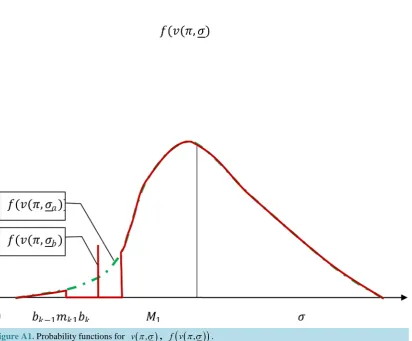
π ∈ =  . It follows that a change of σ from 1 to 0 represents a stochastic shift redistributing risk from π to the quantile means mk₁,k=1,,K . This shift in risk implied by the function v

(

π σ

,

)

is

illu-strated in Figure A1.

For a given σ in (11), let Fv

(

⋅|M₁,

σ

)

be the distribution function of the payoff v

(

π σ

,

)

given in (11). For a given σ ,the effects of changes in mean payoff M₁ on Fv

(

⋅|M₁,

σ

)

represent a horizon shift in the distribution function, holding the distribution of “deviations from the mean” constant. This is used below in our welfare evaluation as any sure willingness-to-pay corresponds to a horizontal shift in the distribution function. Define R_a

( )

σ

as the sure amount satisfying

(

)

(

| 1,

)

(

(

| 1

( )

, 0

)

)

v v

a

VU F ⋅ M σ =VU F ⋅ M −R σ , (12a)

where R_a

( )

σ

is the agent’s willingness to pay to replace the random payoff v

(

π σ

,

)

by v

(

π

, 0

)

. Equation (12a) implies that Ra

( )

0 =0. And Ra

( )

1 measures the willingness-to-pay to replace π by the quantile means

1

k

m ’s, with m_k1 occurring with probability _F b

( )

_k −F b

(

_k−1

)

_,k=1,,K.

For given σ , note that Lemma 1 implies that there exists a distribution function Fvc

( )

σ

such that Equation (12a) can be alternatively written as

(

)

( )

(

, , vc

)

(

(

,0

)

( )

, vc

( )

)

a

E U v_ π σ F σ  =_ E U v_ π −R σ F σ _, (12b)

where v

(

π σ

,

)

is defined in (11), and vc

( )

( ) (

v | ₁,

)

(

1

( )

)

v

(

| ₁

( )

,0

)

a

F σ =β σ F ⋅ M σ + −β σ F ⋅ M −R σ for

some

β σ

( )

∈

[ ]

0,1 .

Next, consider the second step. Letting s∈

[ ]

0,1 , define

( )

, k1

(

1

)

1

w

π

s =sm + −s M when π ∈S kk, =1,,K. (13)

Note that w

(

π

, 0

)

=M₁, and w

( ) (

π

,1 =v

π

,0

)

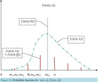
. It follows that a change of s from 1 to 0 represents a redi-stribution of risk from the m_k1’s to the overall mean M₁. This shift in risk implied by the function w

( )

π

,s in (13) is illustrated in Figure A2.

For a given𝑠𝑠 in (13), let

(

| 1,

)

w

F ⋅ M s be the distribution function of the payoff w

( )

π

,s given in (13). Again, for a given s, the effects of changes in mean payoff M₁ on

(

| 1,

)

w

F ⋅ M s represent a horizon shift in

11_{In addition, noting that}

( )

( )

( )

1

1 1

d K K

j

kj k k kj

k k

F P F b F b Q

ππ π =

∑

= =

∑

= − − 

∫

, it follows that the overall j-th (non-central) moment

( )

d

j

F ππ π

∫

is the weighted sum of the j-th quantile (non-central) moment Qkj across all K intervals, with F b( )k −F b( )k−1  as

791

the distribution function. Define R s_b

( )

as the sure amount satisfying

( )

(

)

(

| 1 1 ,

)

(

(

| 1

( )

1

( )

,0

)

)

w w

a a b

VU F ⋅ M −R s =VU F ⋅ M −R −R s , (14a)

where R s_b

( )

is the agent’s willingness to pay to replace the random payoff w

( )

π

,s by w

( )

π

, 0 . Equation (14a) implies that Rb

( )

0 =0. And Rb

( )

1 measures the willingness-to-pay to replace the quantile means

1

k

m ’s by the overall mean M, each m_k1 occurring with probability _F b

( )

_k −F b

(

_k−1

)

_,k=1,,K.

For a given s, Lemma 1 implies that there exists a distribution function Fwc

( )

s such that equation (14a) can be alternatively written as

( )

( )

( )

(

, a 1 , wc

)

(

(

,0

)

a

( )

1 b

( )

, wc

( )

)

E U w_ π s −R F s _=E U w_ π −R −R s F s _, (14b)

where w

( )

π

,s is defined in (13) and

( )

( )

(

| 1

( )

1 ,

)

(

1

( )

)

(

| 1

( )

1

( )

,0

)

wc w w

a a b

F s =β s F ⋅ M −R s + −β s F ⋅ M −R −R s for some

β

( )

s ∈

[ ]

0,1 .

Noting that

(

| 1, 1

)

v

F ⋅ M =F, Fw

(

⋅|M₁,1

)

=Fv

(

⋅|M₁,0

)

, Fw

(

⋅|M₁, 0

)

=H

(

⋅|M₁

)

, and combining (2), (12a) and (14a), we obtain the following result.

Lemma 2: The risk premium R given in (2) can be decomposed as follows

( )

1

( )

1

a b

R=R +R ,

(15)

where Ra

( )

1 and Rb

( )

1 satisfy Equation (12) and Equation (14), respectively.

Equation (15) states that the risk premium R can be decomposed into two additive parts: Ra

( )

1 measuring

the value of moving the risk in each interval to the corresponding quantile means; and Rb

( )

1 measuring the

value of moving the risk from the quantile means to the overall mean. This decomposition will prove useful in deriving a local measure of the risk premium, as discussed below.

3.4. Local Measures

We now proceed with deriving expressions that provide a local approximation of the decomposition of the risk premium given in Proposition 1. Note that, in contrast with the Arrow-Pratt analysis of risk aversion, the lin-kages between local and global characterizations of downside risk aversion are complex. As noted in the intro-duction, Keenan and Snow [14] showed that there is no local measure that can give a global characterization of downside risk aversion. Yet, the local characterization of risk aversion and downside risk aversion remains use-ful as it establishes linkages between the cost of risk and moment-based measures of risk exposure (e.g., [10][12] [13]). Below, we derive local measures of the risk premium expressed across quantiles based on the central moments given in (9)-(10).

Our analysis proceeds first with the local measurement of Ra

( )

1 defined in (12a) or (12b) and then with the

measurement of Rb

( )

1 defined in (14a) or (14b). Under non-expected utility models, our derivations will rely

on (12b) and (14b) and the local utility function U

(

π

,F

)

given in Lemma 1. In this section, we assume that the local utility function U

(

π

,F

)

is three times L_p-Fréchet differentiable on

[

L M,

]

×D12.

Under differentiability, we now present an approximate measure of Ra

( )

1 . (See the proof in the Appendix).

Proposition 2: A local measure of the risk premium component Ra

( )

1 is

( )

(

( )

)

( )

(

)

( )

( )

{

}

( )

(

)

( )

(

)

( )

(

)

( )

( )

{

}

( )

(

)

1

1 2

1

1 1

1

1

1 3

1

1 1

1

, 1

2 _,

, 1

6

0 1

0

0

0 ,

vc k K

a k K vc k k k

i i i

i

vc k K

k k k

k K _vc

i i i

i

U m F

R F b F b m

U m F F b F b

U m F

F b F b m

U m F F b F b

− =

− =

− =

− =

 

 

≅− _{  } ′′ _ − _

  ′ −

′′′

  _{ }

−_{  } −



 

 _{ } 

 

 

 

 _ 

  _ ′ _ − _ _

∑

∑

∑

∑

(16)

12_{Note that this}

p

L -Fréchet differentiability assumption can be relaxed. This may be needed in situations where U

(

π,F

)

has kinks. This can arise in models exhibiting loss aversion (e.g., [2]) or disappointment aversion (e.g., [4]) where the local utility function is continuous in

792 where U′

(

π,F

)

=∂U

∂ ,

(

)

2 2

, U

U π F π ∂ ′′ = ∂ ,

(

)

3 3 , U

U π F π ∂

′′′ =

∂ , mk2 is the quantile variance of π in the interval

k

S , and m_k3 is the quantile skewness of π in the interval S kk, =1,,K.

Equation (16) gives an approximate measure of Ra

( )

1 , the component of the risk premium associated with

replacing π in each S_k by its quantile mean m_k1, where m_k1 occurs with probability

( )

k

(

k 1

)

, 1, ,

F b F b₋ k K

 −  =

   .

An approximate measure of Rb

( )

1 is given next. (See the proof in the Appendix).

Proposition 3:A local measure of the risk premium component Rb

( )

1 is

( )

(

( )

)

( )

(

)

{

( )

( ) (

)

}

( )

(

)

( )

(

)

{

( )

( ) (

)

}

1 2

1 1 1 1

1

1 3

1 1 1 1 1 , 0 1 1 2 , , 1 6 0 0 , 0 wc K

b wc k k k k

wc

K

k k k

k wc

U M F

R F b F b m M

U M F

U M F

F b F b m M

U M F

− = − = ′′   _{  } ≅ −_{  } − _{ } − _ ′   ′′′   _{  } −_{  } − _{ } − _ ′  

∑

∑

(17)

where U′

(

π,F

)

=∂U

∂ ,

(

)

2 2

, U

U π F π ∂

′′ =

∂ and

(

)

3 3

, U

U π F π ∂

′′′ =

∂ .

Combining Lemma 2 with Propositions 2 and 3, we obtain the following key result. Proposition 4: The overall risk premium R can be approximated as

( )

(

)

( )

(

)

( )

( )

{

}

( )

( )

( )

(

)

( )

(

)

{

( )

( ) (

)

}

( )

(

)

( )

(

)

( )

( )

{

}

( )

( )

1 1 2 1 1 1 1 1 2

1 1 1 1 1 1 1 1 1 1 0 0 0 0 , 1 2 _, , 1 2 , 0 6 _, 0 , 1 vc k K

k k k

k K vc

i i i

i

wc

K

k k k

k wc vc k k k K vc

i i i

i

U m F

R F b F b m

U m F F b F b

U M F

F b F b m M

U M F

U m F

F b F b

U m F F b F b

− = − = − = − − = ′′   _{ } ≅ −_{  } − _   ′ − ′′   _{  } −_{  } − _{ } − _ ′          _{ }          ′′′   _{ } −_{  } − _   ′ −

∑

∑

∑

∑

( )

(

)

( )

(

)

{

( )

( ) (

)

}

3 1 1 3

1 1 1 1 1 0 , 0 1 . 6 , K k k wc K

k k k

k wc

m

U M F

F b F b m M

U M F = − = ′′′   _{  } −_{  } − _{ } − _ ′            

∑

∑

(18)

Equation (18) provides an approximate decomposition of the overall risk premium R in terms of the contribu-tion made by each interval S kk, =1,,K. For the k-th interval, it shows the role of risk preferences (where

U U′′ ′

− reflects aversion to variance, and U′′′ ′U reflects aversion to skewness). Note that these results are consistent with previous research. When there is single interval (K = 1), Pratt [16], Arrow [17], and Machina [19]

have identified

(

−U U′′ ′

)

as a local measure of risk aversion. And Crainich and Eeckhoudt [12], Modica and Scarsini [10] and Jindapon and Nielson [13] have shown that

(

U′′′ ′U

)

is a local measure of aversion to down-side risk. By using a quantile approach, our analysis extends this research by identifying the role of risk aversion and downside risk aversion relative to risk exposure in different intervals/quantiles of the distribution (with K

being any integer greater than 1).

Equation (18) also shows how risk exposure across intervals affects the (approximate) cost of risk. It meas- ures risk exposure by the probability of being in the k-th interval _F b

( )

_k −F b

(

_k−1

)

_, the quantile mean m_k1, the quantile variance m_k2, the quantile skewness m_k3, and the terms

[

m_k1−M₁

]

2 and

[

m_k1−M₁

]

3.

793

4. Implications

This section discusses the implications of the quantile-based measures of the risk premium and its decomposi-tion given in Proposidecomposi-tion 4. As noted above, our analysis applies under non-expected utility preferences. This section proceeds in three steps. First, we study the implications of Proposition 4 under general risk preferences. Second, we examine the special case where risk preferences satisfy the expected utility model. Third, we eva-luate how departures from expected utility affect the cost of risk. The analysis provides new information on the role of downside risk exposure and its effects on the risk premium.

Combining Propositions 1, 2, 3 and 4, we obtain the following result. (See the proof in the Appendix). Proposition 5: Let V be the class of functions VU

( )

⋅ that are differentiable and strongly monotonic in payoff. Then, for all VU

( )

⋅ ∈V , the k-th component of the risk premium ΔR_k associated with the k-th interval S_k

can be approximated as

[

]

ΔRk ≅ ΔRak+ΔRbk , (19a)

where

( )

(

)

( )

(

)

( )

( )

{

}

( )

(

)

( )

(

)

( )

(

)

( )

( )

{

}

( )

(

)

1 1 2 1 1 1 1 1 3 1 1 1 , 1 Δ 2 _, , 1 , 6 0 0 0 0 , vc k

ak K vc k k k

i i i

i

vc k

k k k

K _vc

i i i

i

U m F

R F b F b m

U m F F b F b

U m F

F b F b m

U m F F b F b

− − = − − = ′′           _{ } = −_{  } − _   ′ − ′′′   _{ } −_{  } − _   ′ −

∑

∑

(19b)

( )

(

)

( )

(

)

( )

( ) (

)

( )

(

)

( )

(

)

( )

( ) (

)

1 2

1 1 1 1

1 3

1 1 1 1 , 1 Δ 2 , , 1 , 6 0 0 0 , 0 wc

bk _wc k k k

wc

k k k

wc

U M F

R F b F b m M

U M F

U M F

F b F b m M

U M F

− −   ′′   _{ } = −_{  } − _ − ′   ′′′   _{  } −_{  } − _ −     ′   (19c) 1, ,

k=  K.

Equations (19a)-(19c) are consistent with the decomposition of the risk premium R given in (6b) (defining

ΔRk satisfying 1Δ K

k k

R=

∑

₌ R ) and in (15) (defining Ra

( )

1 and Rb

( )

1 satisfying R=Ra

( )

1 +Rb

( )

1 ).

And they are consistent with the approximations given in (16), (17) and (18). As such, Equation (19b) defining

ΔRak can be interpreted as an approximate measure for the part of Ra

( )

1 associated with moving the risk in the k-th interval S_k to the quantile mean mk₁,k=1,,K. It includes two additive terms: a variance

compo-nent (including the quantile variance m_k2), and a skewness component (including the quantile skewness m_k3). Each of these terms is weighted by the probability of being in the k-th interval, _F b

( )

_k −F b

(

_k−1

)

_. The

va-riance component is also weighted by the term

(

( )

)

( )

(

)

( )

( )

{

1 1 1

}

1 , 0 0 , vc k K vc

i i i

i

U m F

U m F F b F b−

=

′′

′ _ − _

∑

, reflecting risk prefe-

rences with respect to variance. Under risk aversion (where U′′

( )

π

<0), this means that an increase in variance in the k-th interval tends to increase the incremental cost of risk ΔR_ak. And the skewness component is

weighted by the term

(

( )

)

( )

(

)

( )

( )

{

1 1 1

}

1 , , 0 0 vc k K vc

i i i

i

U m F

U m F F b F b−

=

′′′



′ _ − 

∑

, reflecting risk preferences with respect to

skewness. Under downside risk aversion (where U′′′

( )

π

>0; see [8]), this implies that an increase in skewness in the 𝑘𝑘-th interval tends to reduce exposure to downside risk and decrease the incremental cost of risk ΔR_ak.

Similarly, Equation (19c) defining ΔR_bk can be interpreted as an approximate measure for the part of R_b

( )

1

associated with moving the risk from the quantile mean m_k1 to the overall mean M k₁, =1,,K. Again, it in- cludes two additive terms: a variance component (including the squared deviation from the mean,

[

m_k1−M₁

]

2,

794

weighted by the probability of being the k-th interval, _F b

( )

_k −F b

(

_k−1

)

_. The variance component is also

weighted by the term

(

( )

)

( )

(

11

)

0

, 0

, wc

wc

U M F

U M F

′′

′ , reflecting risk preferences with respect to variance. Under risk aver-

sion (where U′′

( )

π

<0), this implies that an increase in squared deviation of m_k1 from the mean M₁ tends to increase the incremental cost of risk ΔR_bk. And the skewness component is weighted by the term

( )

(

)

( )

(

11

)

0

0 ,

, wc

wc

U M F

U M F

′′′

′ , reflecting risk preferences with respect to skewness. Under downside risk aversion (where

( )

0

U′′′

π

> ), this means that an increase in cubed deviation of m_k1 from the mean M₁ tends to reduce expo-sure to downside risk and decrease the incremental cost of risk ΔR_bk.

These results provide useful information on the economics of downside risk. To the extent that most decision makers are averse to downside risk, they provide a way to assess the cost of downside risk exposure. First, since our analysis applies to all intervals S_k’s, it clearly applies to the lowest interval S₁. As such, when k=1, Proposition 5 gives a local measure of the cost of risk associated with the low end of the payoff distribution. Assuming the first interval S₁ captures relevant information on downside risk, this measure is useful in eva-luating downside risk aversion. Under downside risk aversion, this is the type of risk exposure that may be of greatest concern (e.g., [6][8]).

Note that our analysis includes the expected utility model as a special case. Indeed, as noted above, the ex-pected utility model holds when U

(

π

,F

)

=U

( )

π

for all F∈D, i.e. when the local utility function U

(

π

,F

)

does not depend on F. Then, the k-th component of the risk premium associated with interval S_k is given by Equations (19b) and (19c) with U

(

π

,F

)

=U

( )

π

, To illustrate, consider the case of expected utility where

(

a b+

π

)

>0,b>0, and U

( )

π

belongs to the class of hyperbolic absolute risk aversion utility function:

( )

(

)

(

)

(

)

1 1

– 1 when 1,

ln when 1.

b

a b b b

U

a b

π π

π ₋     

 ₊  _≠

 

=  

 _{+ =}



(20)

Under (20), we have U′

( ) (

π = a+bπ

)

−1b >0, –U′′

( ) ( )

π

U′

π

=1

(

a b+

π

)

>0, and

( )

( ) (

) (

)

2

1 0

U

b a b

U

π

π

π

′′′ _{ }

= + _ + _>

′ 13. Substituting these expressions into (19b)-(19c) shows how our analysis can be used to provide simple measurements of the component of the risk premium associated with the k-th quantile of the payoff distribution. When focusing on the lowest quantile (k=1), this provides explicit linkages between quantile variance and skewness measures, risk preferences and the cost of exposure to downside risk under the expected utility model. An empirical illustration of the usefulness of the approach is given in Kim et al. [28], which presents a case study documenting the importance of downside risk in the evaluation of the cost of risk.

More importantly, our analysis applies to non-expected utility models. This corresponds to situations where the local utility function U

(

π

,F

)

depends on F. As discussed by Machina [19] and Wang [23], this allows for preferences that are nonlinear in the probabilities, thus relaxing the independence axiom. Our analysis provides new and useful insights on the implications of non-expected utility models for the evaluation of the risk pre-mium. To illustrate, consider the rank-dependent utility model

( )

M

( )

d

(

( )

)

,

RDU _L

V F =

∫

u π G F π

(21) where u:

[

L M,

]

→ is a differentiable and strictly increasing function, and G: 0,1

[ ] [ ]

→ 0,1 is a differenti-able and strictly increasing function satisfying G

( )

0 =0 and G

( )

1 =1. Using integration by parts, (21) can be

alternatively written as VRDU

( )

F =u M

( )

–

∫

_LMG F

(

( )

π

)

du

( )

π which implies that

13_{Following Pratt [16], Arrow [17] and Menezes et al. [8], this satisfies risk aversion (with U}′′

( )

π _{<0) and downside risk aversion (with}

( ) 0

795

( )

–

(

( )

)

( )

RDU

V G u

F

F π F π π π

∂ ₌ ∂ ∂

∂ ∂ ∂ . It follows that, under the rank-dependent utility model (21), the local utility

function U

(

π

,F

)

in (8) can be written as

(

,

)

(

( )

)

( )

d

L

U π F =

∫

πG F y u y′ ′ y, (22)

where G F

(

( )

)

G

(

F

( )

)

0

F

π ∂ π

′ = >

∂ and

( )

( )

0

u

u π π

π

∂

′ = >

∂ . Under differentiability, (22) implies

(

,

)

(

( )

)

( )

,

U′ π F =G F′ π u′ π

(23a)

(

,

)

(

( )

)

( ) ( )

(

( )

)

( )

,

U′′ π F =G′′ F π F′ π u′ π +G F′ π u′′ π

(23b)

where

(

( )

)

(

( )

)

2 2

G

G F F

F

π ∂ π

′′ =

∂ ,

( )

( )

0

F

F π π

π

∂

′ = ≥

∂ and

( )

( )

2 2

u

u π π

π ∂ ′′ =

∂ ,

(

)

(

( )

)

( )

( )

(

( )

)

( ) ( )

( )

(

)

( ) ( )

(

( )

)

( )

2

, 2

,

U F G F F u G F F u

G F F u G F u

π π π π π π π

π π π π π

′′′ = ′′′ _ ′ _ ′ + ′′ ′ ′′

′′ ′′ ′ ′ ′′′

+ + (23c)

where

(

( )

)

(

( )

)

3 3

G

G F F

F

π ∂ π

′′′ =

∂ ,

( )

( )

2 2

F

F π π

π ∂ ′′ =

∂ and

( )

( )

3 3

u

u π π

π ∂ ′′′ =

∂ . Equations (23a)-(23c) give the derivatives of the local utility function U

(

π

,F

)

associated with the rank dependent utility model (21). Substi-tuting these expressions into (19b)-(19c) provide simple measurements of the (approximate) component of the risk premium associated with the k-th quantile of the payoff distribution. When focusing on the lowest quantile (k=1), this provides linkages between quantile variance and skewness measures, risk preferences and the cost of exposure to downside risk under the rank-dependent utility model (21).

Of special interest here is the case of risk preferences that tend to “overweight” the probability of rare events located in the lower tail of the distribution (e.g., [2]). As noted by Quiggin ([20][24]), Schmeidler [33], Gonza-lez and Wu [36] and others, this oversensitivity to the probabilities of unfavorable events is consistent with the function G

( )

⋅ in (21) being strictly concave in the interval

[ ]

L k, for some k∈

(

L M,

)

. When S1⊂

[ ]

L k, ,

it means that G′′

(

F

( )

π

)

<0 for π ∈S₁. Equation (23b) then implies that U′′

(

π,F

)

<G F′

(

( )

π

)

u′′

( )

π when

1

S

π ∈ . In this case, compared to the expected utility model (obtained as a special case of (21) when

( )

(

)

1

G F′ π = ), oversensitivity to rare unfavorable events makes the term U′′

(

mk₁,F

)

more negative. From

(19b), this gives an important result: for a risk averse decision maker (with U′′

(

π

,F

)

<0),”overweighting” the probability of rare events located in the lower tail of the distribution tends to increase the effect of the quantile variance m12on ΔRa1. The quantile variance m12 in the interval S1 is a measure of exposure to downside risk.

We have shown in Proposition 4 and Proposition 5that ΔR_a1 is a component of the risk premium R. Thus, der risk aversion, our analysis indicates how exposure to downside risk interacts with the sensitivity to rare un-favorable events to increase the risk premium. In particular, our results document how a departure from the ex-pected utility model in the interval S1 can contribute to increasing the risk premium.

Finally, our investigation also provides useful information on how quantile skewness affects the risk premium. To see that, rewrite Equation (23c) as

(

)

(

( )

)

( )

(

( )

)

( )

( )

(

( )

)

( ) ( )

( )

(

)

( ) ( )

2

, 2

.

U F G F u G F F u G F F u

G F F u

π π π π π π π π π

π π π

′′′ − ′ ′′′ = ′′′ _ ′ _ ′ + ′′ ′ ′′

′′ ′′ ′

+ (23c’)

Comparing the rank dependent utility model (21) with the expected utility model (obtained when

( )

(

)

1