PID Controller Tuning in Reverse Osmosis System based on Particle Swarm Optimization

PID Controller Tuning in Reverse Osmosis System

based on Particle Swarm Optimization

K.Chithra¹, Dr.Andy Srinivasan², V.Vijayalakshmi³, A.Asuntha4 1

PG Student [C&I], Dept. of EIE, Valliammai Engineering College, Chennai, Tamil Nadu 2

Professor, Dept. of EIE, Valliammai Engineering College, Chennai, Tamil Nadu2 3

Assistant Professor, Dept. of EIE, Valliammai Engineering College, Chennai, Tamil Nadu3 4

Assistant Professor, Dept. of EIE, SRM University, Chennai, Tamil Nadu 4

Abstract: The water scarcity is one of the major problems for the global issues for long days. The main objective of the present work is to utilize a simplified model to predict the performance of Reverse Osmosis unit. The optimization techniques such as Particle Swarm Optimization (PSO) and Genetic Algorithm (GA) are used in order to overcome these problems but it needs long computation time, any how we can easily tune the parameters when compared to other conventional techniques. This paper describes about the Reverse Osmosis (RO) system based on decoupled design and PID controller tuning based PSO.

Keywords: Reverse Osmosis (RO) plant, PID tuning Membrane, Particle Swarm Optimization (PSO), Genetic Algorithm (GA)

I. INTRODUCTION

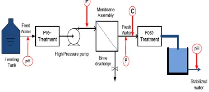
Reverse Osmosis is a water separation process used to demineralize water or desalt sea water [1]. Since RO process is the multivariable system we need to control major parameters such as Pressure, pH, flux and conductivity, to analyze the plant outputs. Reverse osmosis is one of the filtration process based on membrane [10]. The membrane assembly has made up of

cellulose acetate [2]–[4]. Pressure is applied to the input feed side through high pressure pump. Feed water is sent before pre-treatment process, and then we need to check the pH level. The major problems of existing plant are bio-fouling, scaling formation and concentration due to the high pH value. So we need to replace the membrane because the membrane life is reduced [7]. To overcome these problems pH values is adjusted at the feed side and the impurities are controlled by changing the conductivity values. Computer Simulation in terms of a virtual process is designed to check the algorithm and compare the results with Ziegler-Nichols method and PSO. The PSO shows better control performance than Ziegler-Nichols tuning method in both qualitatively and quantitatively as well.

II. THE REVERSE OSMOSIS MODEL

The general Reverse Osmosis plant diagram is shown in the Fig. 1. RO system consists of four major components.

Fig. 1: Reverse Osmosis system

Technology (IJRASET)

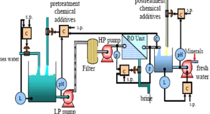
The main objective of this RO process is maintaining a constant production rate at which acceptable purity. The permeate flux and conductivity are affected by pH, pressure and temperature [5]. To optimize the membrane salt rejection and to prevent alkaline scale perception due to pH value adjustment of pretreatment process. The feed water temperature affects the water flux in another way. If the RO plant is operating under an ideal condition with no fouling or scaling, water flux will decline with time, because of compaction phenomena [14]. The water flux though the membrane is directly proportional to the pressure drop across the membrane. Since the pressure at the product side is constant, it follows that the water flux is directly related to the feed pressure. Fig. 2 shows the control loops of the RO plant.

Fig. 2: Control loops of the RO plant

Generally manipulated variables affect more than one controlled outputs. One approach to handling this problem is known as decoupling. This decoupling is not always possible without a notable performance degrading [5]. In order to overcome this problem, a new approach has proposed and it will be applied in this work.

IV. PLANT MODELING

Transfer function of the Ro system can be represented as equations (1) to (5). The model equations used in the RO system is taken from Doha Reverse Osmosis Plant (DROP) [3].

=

G

_G

G

_G

(1)

G

=

=

. .

(2)

G

=

= 0

(3)

G

=

=

. .

(4)

G

=

=

. .

(5)

where,

P=Pressure, Kpa (psig)

P =Density of H ion F=Flux, gpm (m³/s) C=Conductivity (µs/cm)

The linear approximation ranges as shown in table 1.

Table 1: Ranges for Linear Approximation

VARIABLE LINEAR RANGE

Flux, gpm(m/s) 0.85-1.25(0.2-0.3)

Pressure, Kpa(psig) 800-1000(5500-7000)

Conductivity( µs/cm) 400-500

©IJRASET 2015: All Rights are Reserved

353

Model design of the RO membrane has mainly affect with pH control and conductivity of the water. The model design of the RO membrane assembly is shown in Fig. 3.

Fig. 3: Model design of the RO membrane

The model design of Ro membrane effect with pH value as well as the conductivity value of the water. Here the membrane assembly should become the open loop stable. When there is high value means that, it will affect the loss of efficiency and scaling formation on the membrane.

VI. CONTROL SYSTEM DESIGN

The manipulated variable is pressure and pH. In the reverse osmosis system plant has one manipulated input variable affects the more than one control output. Here the DROP system is taken which is MIMO system and it should be open loop system is stable [7]. The inputs are affected by manipulated inputs. Fig. 4 shows the total decoupled system structure.

Fig. 4: Decoupled system structure

where,

G _{( )}=− (6)

G _{( )}=− (7)

The total structure for the RO system is stable because each subsystem of the block is open loop stable because each have negative real pole.

Technology (IJRASET)

©IJRASET 2015: All Rights are Reserved

354

Particle swarm optimization first introduced by Kennedy and Eberhart in 1995. It is the most advanced optimization technique using today. The aim of optimization is to determine the best-suited solution to a problem under a given set of constraints. Several researchers over the decades have come up with different solutions to linear and non-linear optimization problems. Mathematically an optimization problem involves a fitness function describing the problem, under a set of constraints representing the solution space for the problem [4]. The velocity of the particle is changed according to the relative location of positionand velocity. The following equation is used to update the particle velocity.

v( )= wv( )+ c ∗rand()∗ pbest −x( ) + c ∗rand()∗(gbest −x( )) (8)

x( )= x( )+ v( ) (9)

j =1, 2…….n and g=1, 2……..m where,

n= number of particle in group m= number of members in a particle t=pointer of iterations (generations)

v( )=velocity of particle j at iteration t, v ≤ v( )≤ v

w = inertia weight factor

c , c = acceleration constants rand () = random variable

x( ) = current position of particle j at iteration t

pbest = p best of particle j

gbest = g best of group upto k iterations

The best previous value of the jth particle is saved and can be represented as pbest = (pbest , pbest , pbest , … . . pbest ). Now comparing the fitness of each particle with fitness of the global optimal position called as gbest is passed in the population as the current current global optimal position gbest. Velocity of the jth particle change is represented by

©IJRASET 2015: All Rights are Reserved

355

A scheme of controller tuning was proposed by Shi and Eberhart in which inertia term is weighted by a weighting factor which is given by following equation

w = w = {w −w |itr }*itr (10)

Start

Initialize particle with random position

Set pbest=p

Calculate the random position

If fitness (p) better than fitness pbest

If fitness (p) better than fitness gbest

Is optimum

Update particle’s position and velocity

Stop

Yes

Yes

Yes

No

Technology (IJRASET)

w = 0.9 and w = 0.4

The value of “inertia weight” is large at beginning but gradually it becomes smaller as the number of iterations increases. The velocity and the position update according to equation from (9) and (10).

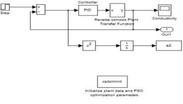
G11 is the MIMO system for flux control. It is simulated in MATLAB for obtaining a flux control through by changing the values of the PID controller we can get continuous oscillation.The flux of water is controlled to be within the range of 0.85-1.25 (m /s) by the PSO based PID controller tuning which is shown in the above Fig. 6.

Kp=Proportional Gain= 0.7022

Ki=Integral Gain= 0.001

Kd= Derivative Gain= 0.4440

By applying these values to PID controller for PSO we can get the desired output flux.

Fig. 6: PID controller tuning for flux

G22 is the MIMO system for conductivity control. It is simulated in MATLAB for obtaining a conductivity control through by changing the values of the PID controller we can get continuous oscillation.The conductivity of water is controlled to be within the range of 400-500 (μs/cm) by the PSO based PID controller tuning which is shown in the above Fig. 7.

Kp=Proportional Gain= -0.0225 Ki=Integral Gain= -0.02 Kd= Derivative Gain= -0.05

By applying these values to PID controller for PSO we can get the desired output flux.

©IJRASET 2015: All Rights are Reserved

357

Ziegler-Nichols tuned PID controlled RO plant system produces response for Flux and conductivity. This system produces high overshoot, rising time and settling time. To overcome these difficulties, I have used PSO based PID controller tuning and this method gives the better response for the RO plant when compared to Z-N method. In the conventional Ziegler-Nichols tuned PID controller, the RO plant system response for Flux and conductivity produces high overshoot, rising time and settling time. But using PSO based PID controller tuning gives the better response for the system. In the present, comparison is made with result of Ziegler-Nichols PID tuning and PSO based PID tuning as shown in table 2.

Table 2: PID gain comparison

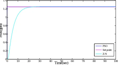
A comparison of time domain performance specifications peak overshoot, rise time and settling time for flux control response is shown in Fig. 8.

Fig. 8: Comparision of servo response for flux

A comparison of time domain performance specifications peak overshoot, rise time and settling time for flux control values are tabulated in table 3.

Scheme Z-N PSO

Performance index (ITAE)

0.03 0.232

Rise time (sec) 12860 27.3

Settling time(sec) 9418 42.3

Final value 1.25 1.25

Table 3: Comparision of Performance for Flux

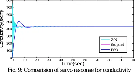
A comparison of time domain performance specifications peak overshoot, rise time and settling time for conductivity control response is shown in Fig. 8. PSO based PID tuning method has the lower gain when compared to Z-N tuning method as shown in Fig. 8. As same as the PSO based PID controller tuning using the performance of flux range is 0.85-1.25 (m /s) shown in Fig. 9.

As seen from this response Fig. 8 the present technique gives the better response in terms of overshoot, rising time and settling time.

0 10 20 30 40 50 60 70 80 90 100

0 0.2 0.4 0.6 0.8 1 1.2 1.4 Time(sec) F lu x (g p m ) PSO Set point Z-N System Ziegler-Nichols

P I D

PSO

P I D

499 0.004 0.002 0.7022 0.001 0.4440

Technology (IJRASET)

©IJRASET 2015: All Rights are Reserved

358

A comparison of time domain performance specifications peak overshoot, rise time and settling time for conductivity control values are tabulated in table 4.

Table 4: Comparison of performance for conductivity

Scheme Z-N PSO

Performance index (ITAE) 0.903 0.32

Rise time (sec) 0.116 0.02

Settling time(sec) 3.90 3.61

Peak Overshoot (%) 76.93 46.61

Final value 430 430

IX. CONCLUSION

In this paper, analyses has been done with the Reverse Osmosis system, using decoupled system using the MATLAB-SIMULINK software tool is used for finding the behavior of flux and conductivity for reverse osmosis membrane. From the response curve, we can see that the conductivity changes as a result of pH values; however the flux is not affected because of the changes in pH values. So the conductivity is controlled with the pH and flux is controlled with the pressure. A computer is done to see the results for the flux and conductivity using Ziegler-Nichols based and PSO based PID tuning, Comparing the system response using proposed technique are far better improved. Since lots of non-linearity’s and uncertainties in the real plant has not taken in this study, implementation of PSO to real plant is being scheduled.

X. FUTURE SCOPE

In future, we would like to extend our project using Genetic Algorithm (GA) and Model Predictive Control (MPC) with compare the present results.

REFERENCES

[1] M.W. Robertson 1, J.C. Watters 1., P.B.Desphande 1, J.Z. Assef 1, and I.M. Alatiqi 2, “Model based control for reverse osmosis desalination processes”, Desalination 104 (1996) 59-68.

[2] Abderrahim Abbas, “model Predictive control of a reverse osmosis Desalination unit”, Desalination 194(2006) 268–280.

[3] C. Riverol1 and V. Pilipovik2 ,“ Mathematical Modeling of Perfect Decoupled Control Systemand Its Application: A Reverse Osmosis Desalination Industrial-Scale Unit” , Journal of Automated Methods & Management in Chemistry, (2005), no. 2, 50–54.

[4] Natwar S. Rathore, NehaKundariya, AnirudhaNarain “PID Controller Tuning in Reverse Osmosis System based on Particle Swarm Optimization” International Journal of Scientific and Research Publications, Volume 3, Issue 6, June 2013 1 ISSN 2250-3153.

[5] Jimo Park, Goeun Kim, Jinsung Kim, Sanggun Na and HoonHeo” Simulation of reverse osmosis plant using RCGA based PID controller” ICROS-SICE International Joint Conference August 18-21, 2009J.

[6] Jin-Sung Kim, Jin-Hwan Kim, Ji-Mo Park, Sung-Man Park, Won-Yong Choe, and HoonHeo “Auto Tuning PID Controller based on Improved Genetic Algorithm for Reverse Osmosis Plant” International Journal of Electrical and Computer Engineering 3:8 2008.

[7] Kennedy and R.C.Eberhart, “Particle Swarm Optimization,” in Proceedings of the IEEE International Conference on Neural Networks, vol. 4, pp. 1942– 1948, Dec 1995.

[8] Y.Shi and R.Eberhart,”A modified particle swarm optimizer”, in Proc. IEEE World Congr.Comput.Intell., 1998, pp. 69-73.

[9] S. M. Giriraj Kumar, Deepak Jayaraj, Anoop. R. Kishan, “PSO based tuning of a PID controller for a high performance drilling machine”, International Journal of Computer Applications(0975-8887), Volume 1, No. 19, 2010.

[10] KhawlaAbdulMohsen Al-Shayji, “Modeling, simulation, and optimization of large-scale commercial desalination plants”, Faculty of the Virginia Polytechnic Institute and State University, a PhD Thesis.

0 10 20 30 40 50 60 70 80 90 100