A Mobile Robot Path Planning Based on Multiple Destination points

A Mobile Robot Path Planning Based on Multiple Destination-points

Jing-jing WANG, Xi-sheng DAI and Ke-ne LI

School of Electrical and Information Engineering, Guangxi University of Science and Technology, Liuzhou Guangxi 545006, China

*Corresponding author

Keywords: Mobile robot, Path planning, Multitasking.

Abstract. Path planning is an important aspect of mobile robot. This paper mainly studies the

global path planning with multiple sub-path targets. Firstly, this paper build two initial distance matrix, then construct a minimum distance matrix by Dijkstra algorithm. Finally, the paper determine the destination nodes which have all minimum path. The path planning method can be used to some service robots, including: family service robots, medical robots, industrial robots.

Introduction

Path planning is an important issue in the technical and research field of mobile robots. Path planning means that in the environment with obstacles, the mobile robot should find out an optimal path according to certain evaluation criteria (such as minimum energy, shortest routes, shortest running time, etc.) [1,2]. In general, the environment can be divided into two types: (1) global path planning which refers to find out the optimal path from the starting point to the target point based on a priori model of the environment, in which obstacles are mostly static; (2) local path planning which means that the work environment is unknown or partly unknown, and the mobile robot needs to acquire some unknown information (such as sizes, shapes, locations, and etc.) of obstacles by the sensor array, and generate the optimal path in real-time [3-5].

There are many ways to study path planning. The traditional path planning methods include: Visibility Graph, C-Space Method, Grid Algorithm, Artificial Potential Field Theory, Topological Method, etc. [6]. With the development of modern computing technology, intelligent algorithms have been widely used in the path planning of mobile robots. Genetic Algorithm [7], Fuzzy Logic Algorithm [8], Neural Network Algorithm [9], Ant Colony algorithm [10], and their combination have been applied in path planning effectively. At present, these methods are mainly studied that finding a optimal path from the starting point direct to the ending point. However, in practical applications, mobile robots may be required to go to a number of different places to complete the task before reaching the designated area. The path planning studied in this paper differs from other paths in that the mobile robot must pass through other specified target points before it reaches the designated location.

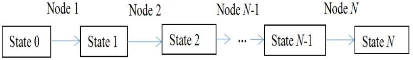
In this paper, an issue on path planning with multiple destination-points is presented and discussed in the environment where the number and vertex-coordinates of obstacles are known. The path planning with multiple destination-points is divided into a number of processes. As shown in Figure 1, the starting point is the state 0, the next target-point is the state 1, the final goal point is the state N, with N =0, 1, 2, …. Each node is a mobile robot task state. A mobile robot moves from one state to another decision-making state. Moreover, the path the mobile robot goes along is the minimum distance between the two states.

Establishment of the Initial Node Distance Matrix

The distance of initial node is mainly consideration of the connection between two points. If the connection between two points does not intersect any obstacle, or not in the obstacle, it can be indicated as a direct straight-line link between two points and the initial distance is the Euclidean distance; In contrast, if the two points can not be directly linked, the initial distance can be assumed infinite. For the two types of adjacency relationship problems solving, an initial distance matrix is established based on the same obstacle’s polygon vertices adjacency relationship and the different obstacles’ polygon vertices adjacency relationship [11]. However, the problem of the two types of adjacency relationships can be solved by judging all the vertex-linkage line of V intersecting with the obstacle polygon, with V being a set of all vertices of the obstacle polygons, together with the initial and final points, i.e., V {v₁,v₂,,v_i,,v_n}. In addition, for the purpose of computing of the distance between vertices, an initial node distance matrix is established as _ERnn_{, with its}

element eij representing the Euclidean distance between vi and vj, the scalar n being the number of

all the nodes (including obstacle vertices, the starting point and destination point). For the details, the initial node distance matrix E can be established with the following situations.

If vi and vj are two adjacent vertices of the same obstacle with their coordinates assuming (x , y_{i i})

and (x , y_{j j}) respectively, then

2

2 _{( )}

)

( _{i j i j}

ij x x y y

e     i, j = 1,…, n. (1)

If vi and vj are two vertices of two different obstacles respectively, the vertex-linkage line of vi and

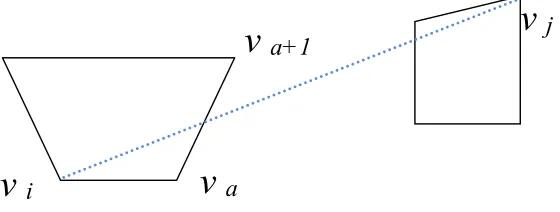
vj needs to be determined that whether it is intersected with any obstacle polygon.

Figure 2. Obstructions within two.

As shown in Figure 2, a vector equation with arbitrary real numbers  and  can be constructed as Eq. (2) to determine if the vertex-linkage line of vi and vj intersects with obstacles,

where va and va+1 are two adjacent vertices of any one obstacle in the environment map.

1

-

-i j i a a a

v （v v） v （v_ v）

(2)

It can be changed to another form as follows.

1

1- vivj 1- vava

（ ） （ ）

(3)

If α, β [0,1], it indicates that the vertex-linkage line intersects with the obstacle, and the corresponding element of the initial node distance matrix is set as

1000 

ij

e _{Intersecting (4)}

v

i

v

j

v

a

2

2 _{( )}

)

( i j i j

ij x x y y

e    

Disjoint (5)

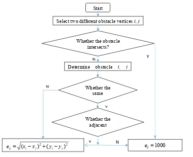
The algorithm flow chart is presented in Figure 3. After all the vertices execute the above operations, the initial node distance matrix E is generated for the given environment map.

Establishment of the Minimum Distance Matrix

Dijkstra algorithm is widely used in finding the shortest path from a starting point to other vertices [12-14] . The advantage of the algorithm lies in finding out the vertex closest to the starting point, automatically taking it as the new starting point (knee point), and updating the original path information simultaneously. In this paper, an improved Dijkstra algorithm [15] can find out the minimum distance matrix between two points. The method to solve this problem can be divided into three steps. The main computation procedure of Dijkstra algorithm is described as follows.

Step One:

According to the above method, the initial node distance matrix E is established firstly. Here construct a shortest path matrix F, _FRnn_{, row vector}

i

f represent the minimum distance from

other points to point i, element f_ij is the shortest distance from point i to point j. If assuming the starting point is vertex v1, the initial path distance information of the first row e₁ of the matrix

E can be calculated. For programming realization purpose, an one-dimension array S

 

Figure 3. Method of initial distance.

created for recording the information of the minimum-distance point of all the calculated points from the starting point. For example, if vertex i is the minimum-distance point from the starting point, the value corresponding to this point is revised to 1, i.e., S[i]1. Otherwise, S[i]0. In the

Select two different obstacle vertices i, j

Whether the obstacle intersects?

1000 

ij

e  

Determine obstacle i, j

Whether the same

Whether the adjacent

2

2 _{( )}

)

( _{i j i j}

ij x x y y

e      

Y 

N

Y N

Y

beginning, the one-dimension array is initialized as

S

[

n

]



{1,0,



,0}

The computation procedure used to find the nearest point from the new starting point can be described as follows.

for (j = 0; j <n; j ++)

{ if (!S[j])

{If (F[1][j] < min) //here, variable min represents the minimum distance.

{pointv = j; min = F[1][j] ; } //variable pointv represents the minimum-distance point.

}

} Step Three:

for (w = 0; w < n; w++) // update the current path and the shortest distance

{ if (!S[w] && (min + E[pointv][w] < F[1][j]))

{F[1][j] = min + E[pointv][w];

prev[w]=pointv;

}

}

After all nodes complete the minimum-distance computation to point 1, row vector f₁ is obtained and all elements of the array S are 1. The element of f1 is the minimum-distance from

other points to point 1. The following program segment can be executed to find the nodes from t

to 1.

while (prev[m]! = 1)

{printf ("% d \ t", prev[t]); m = prev[m];}

At the same time, according to the above method, the shortest distance is obtained about all the nodes to other points. Minimum distance matrix F is obtained.

Find the Multiple Destination-points Optimal Path

There are t tasks node in mobile robot intermediate tasks (tn). Taking into account the fact that

t t R

P_ (-2)! _{, QR}(t-2)!1_{, (t-2)!12(t-2). Each line in P stores the order of tasks node.}

For example, the j row, it is assumed that i₀ is the initial point and the turn of task nodes are

1 -2 1,i , ,it

i  , qj is the total cost of the j row:

0 1 1 2 t 2t1

j i i i i i i

q  f  f   f _{ } (6)

The length of the optimal path is

1 2)! -, 0,1, = , min

= q j t

L _j （ ₍₇₎

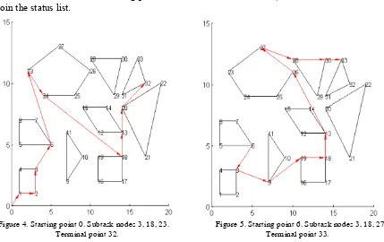
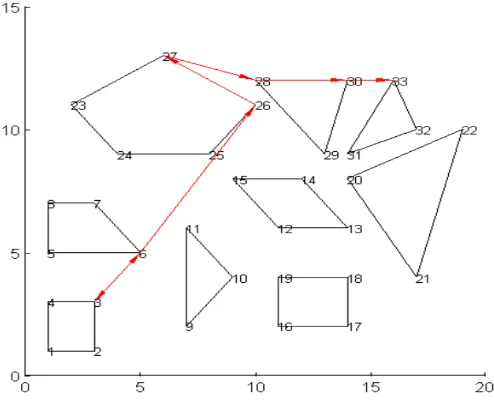
Algorithm can be implemented as a starting point for any point of mobile robot path planning. In Figure 4, the starting point is 0. 3, 18 and 23 are sub-tasks node. Terminal point is 32, the optimal path as shown, the total path length L = 33.380. In Figure 5, the starting point is6, sub-tasks nodes are 3 , 18 and 27. Terminal point is 33, the total path length L= 37.027.

If it is from the state t to the state t + 1, q state need to be repeated, then the state point q does not require to rejoin the list of states. For example, now the robot is at node 3, the next task is at node 26. If intermediate decision-making process needs to be at the node 6, the node 6 does not need to rejoin the status list. 

Figure 6. Starting point 6. Subtask nodes3, 27. Terminal point 33.

Conclusions

In this paper, it is different from one to one point (a starting point directly to the target point) path planning, but for the sub-path planning of intermediate multiple target point. And it is similar to TSP problem [16-18] ( TravellingSalesman Problem) that path planning goes through a number of points. The difference lies in that, in the TSP, each node must traverse only once. But in this paper, according to the actual need, some nodes need to be traversed many times (Figure 6), and some nodes do not need to be traversed. In the TSP Problem, the ultimate goal point must be starting point, but in the paper, the path planning target point may be arbitrarily selected.

Acknowledgement

This work was financially supported by Ph. D Start-up Foundation of Guangxi University of Science and Technology (no. 12Z05), and also Colleges and Universities Key Laboratory of Intelligent Integrated Automation (no. 201502).

References

[1] Guan-wei Wei, Meng-yin Fu, An algorithm based on neural network for mobile robot path planning [J]. In Chinese. Computer simulation. 2010, 27(7): 112-116.

[2] Da-qi Zhu, Ming-zhong Yan. Survey on technology of mobile robot path planning [J]. In Chinese. Control and Decision.2010, 25(7): 961-967.

[3] Wang M., Shan H., Lu R., et al. Real-Time Path Planning Based on Hybrid-VANET-Enhanced Transportation System [J]. IEEE Transactions on Vehicular Technology, 2015, 64(5): 1664-1678. [4] Xing Jun, Wang Jie, Application research of artificial neural network in robot trajectory planning [J]. In Chinese. Micro computer information. 2005, 21(11): 110-111.

[5] Zhang Guo-liang. Survey on Path Planning for Mobile Robot under Dynamic Environment [J]. In Chinese. 2013, 41(1): 157-162.

path planning for intelligent autonomous mobile robot. [J]. Inventi Rapid Algorithm, 2012.

[8] Zoumponos G.T., Aspragathos N.A. Fuzzy logic path planning for the robotic placement of fabrics on a work table [J]. Robotics and Computer-Integrated Manufacturing, 2008, 24(2): 174-186.

[9] Ni J., Li X., Fan X., et al. A dynamic risk level based bioinspired neural network approach for robot path planning [C]// World Automation Congress. IEEE, 2014: 829-833.

[10]Xu Q.L., Zhang D.X. Ant Colony Optimization Algorithm for Robot Path Planning [C]// International Conference on Electrical, Automation and Mechanical Engineering. 2015.

[11]Dai Guang-ming, Li Qing-hua, Research on Algorithm for Avoidance Obstacle Path Planning [D]. In Chinese. Huazhong University of Science and Technology. 2004.

[12]Yuan Bin, Liu Jian-sheng, Analysis of routing planning in logistics network based on improved Dijkstra algorithm [J]. Manufacturing automation. 2014, 5: 103-105.

[13]Murota, Kazuo, Shioura, Akiyoshi. Dijkstra's algorithm and L-concave function maximization [J]. Mathematical Programming, 2014, 145(1): 163-177.

[14]Jacobs B. Dijkstra and Hoare monads in monadic computation [J]. Theoretical Computer Science, 2015, 604: 30-45.

[15]Li Ping. The improvement and implementation of Dijkstra algorithm [J]. In Chinese. Information construction. 2016, 02: 345.

[16]Ying Li, Kai Ma, Jiong Zhang. An Efficient Multicore Based Parallel Computing Approach for TSP Problems [J]. In Chinese. 2013: 98 -104.

[17]Englert M., Röglin H., Vöcking B. Worst Case and Probabilistic Analysis of the 2Opt Algorithm for the TSP [J]. Algorithmica, 2014, 13(1): 190-264.