Study of Weld Component Fatigue Life in Random Environment

© 2017, IRJET | Impact Factor value: 5.181 | ISO 9001:2008 Certified Journal

| Page 3485

STUDY OF WELD COMPONENT FATIGUE LIFE IN RANDOM ENVIRONMENT

Yogesh Nevagi

_{, Kiran Kattimani}

1

_{PG student, Department of mechanical engineering, GIT, Belgaum, KARNATAKA, INDIA}

---***---Abstract - F

random vibrational environment has been carried out in this work. To do so, initially collecting random inputs from the source, requires data acquisition system (DAQ) with the help DAQ, time domain signals from the source are collected; these signals are processed to frequency domain signals to find out the power spectral density (PSD) of the input system. Next phase of the project involves geometrical variation in the weld properties. This exercise yields numbers of combinations; but carrying out analysis and modeling on each of them is time consuming, here modeling exercise is optimized using configuration feature technique and analysis efforts are optimized with the help of design of experimental approach, Taguchi Method.

Further, optimized input results are processed to carry out the random analysis of each of the nine samples selected form the Taguchi optimization method with PSD as an input, with the help of these input Stresses are acquired for the system. Next step is to find out accumulative damage factor of the systems and their by predicting remaining life cycles for the component. With help of results acquired for various geometries efficient component is selected to be in the practical environment. Overall these efforts set a procedure to collect variable input, optimize modeling exercise, choosing best samples amongst the set of all combinations and predicting accumulative damage using probabilistic approach.

Key Words: random vibration, weld component, fatigue life, Power Spectral Density, Data Acquisition System, Taguchi Method

1. INTRODUCTION

This All components in dynamic conditions always tend to experience variable loading during its life cycle span. To be illustrative for such an environment is, transportation machineries like automobiles travelling on rough road surfaces, arbitrary load impact experienced by the industrial equipment’s, bulky static structures having dynamic arrangement in the localized zone facing earthquakes. During static loading conditions input loads are easier to assign i.e. either based on the total weight experienced by the structure under consideration, or impact force; this is static environment scenario. But when it comes to random loading as explained in the examples, extracting the loading pattern is not straight forward and cannot be easily extracted from the source by traditional measuring equipment’s. Inputs are therefore collected in terms of spectrum or also known frequency domain loading. When

the input is in terms of static loading, single force is acting at a time; but in the case of random loading multiple forces acts at the same time. This is the situation which causes difficulty in terms of measurement. So now a question comes how to simplify these inputs to have easiness in the signal conversation though not the measurability. These processes can be easily explained by traditional examples from physics. The laser beam which contains single frequency can be compared with the static loading. Similarly when it comes to the random loading, we have an option called as white light, which does have number of frequencies. How do we analyse the white light? Yes it is by the spectrum, which disintegrates entire frequency pattern. In the mechanical terms, random loading is converted to frequency domain, and this is done by the technique known as the Power Spectral Density. These inputs are processed to analyse the component life in terms of cumulative damages, which plays an important role in the prediction of fatigue life of random environment. This complex environment also creates challenges when physical or environmental changes occur onto the component under consideration. For example a structure is excited to random loading which is either welded, bolted or experiencing environmental challenges like thermal fatigue; it very important to understand the life of the component, number of random variations structure has undergone, so that fatigue failure is predicted, monitored, controlled.

Present work contribute towards the measurement of the random inputs from the generation source, changing the geometrical parameters which can be controlled by the process and are important in deciding the structural stability of the component, optimizing them for design improvement. This is done by random analysis to find out the stresses generated in the system. Further this data is calculated for the cumulative damages to find out the fatigue life of the component.

2. PROBLEM STATEMENT

© 2017, IRJET | Impact Factor value: 5.181 | ISO 9001:2008 Certified Journal

| Page 3486

safety of the product and thereby avoiding dependent loss of important assets like life, time, money etc.

The danger of a catastrophic fatigue failure in the structure may be eliminated/suppressed after knowing the criticality of the welding zones or can help of monitor the situation instead of sudden failure; by designing the structure to have a safe life or to be fail-safe. A proper methodology has to be set to predict the catastrophic failure of weld joints due to fatigue failure in random environment.

3. GEOMETRY OF THE WELD

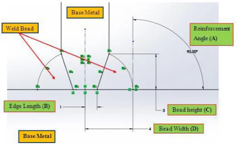
Geometric modeling is carried out by using Solid-Works 15 software .Geometric dimensions and CAD model of weld under consideration are shown below. All dimensions are in mm and angle is in degree. Weld geometry is defined by the various characteristics; below image demonstrate the few of them, these can be controlled by the operator or by specially designed machine. Here the sketch at T section is controlled by the weld reinforcement angle.

Fig - 1:View defining Geometrical variable

3.1 Selection of Sample Using Taguchi Method

These parameters are formulated in terms of Orthogonal Array to determine samples. Here reinforcement angle is assigned with A, weld preparation edge from the center is defined as B, weld bead height indicated as C and its width as D. All these factors have three levels and tabulated in the Table-1.

Table -1: Parameters and variables for experiment

Level/ Factor

A (Reinforcement

angle)

B

(Base) (Height) C (Width) D

1 90 1 3 3.5

2 100 1.25 3.5 4

3 105 1.5 4 5.5

Table -2: Orthogonal array for 3-level, 4Factor

Experiment Reinforcement angle (A)

Base

(B) Height (C) Width (D)

1 A1 B1 C1 D1

2 A1 B2 C2 D2

3 A1 B3 C3 D3

4 A2 B1 C2 D3

5 A2 B2 C3 D1

6 A2 B3 C1 D2

7 A3 B1 C3 D2

8 A3 B2 C1 D3

9 A3 B3 C2 D1

Table -3: Orthogonal array for Parameters and variables under consideration

Experiment Reinforcement _{angle (A)} Base _(B) Height _(C) Width _(D)

1 90 1 3 3.5

2 90 1.25 3.5 4

3 90 1.5 4 5

4 100 1 3.5 5

5 100 1.25 4 3.5

6 100 1.5 3 4

7 105 1 4 4

8 105 1.25 3 5

9 105 1.5 3.5 3.5

3.2 Material properties for base metal and filler metal

Table -4: Material properties for Base metal & Filler metal

Material E

GPa Poisons ratio MPa σt MPa σy g/cmρ 3

Base- Steel

AS36 70 0.29 449 324 2.78

Filler-Steel

© 2017, IRJET | Impact Factor value: 5.181 | ISO 9001:2008 Certified Journal

| Page 3487

4. ACQUIRE PSD (POWER SIGNAL DENSITY)

SIGNALS FROM DAQ (DATA ACQUISITION SYSTEM)

AND FINITE ELEMENT ANALYSIS:

Fig - 1:View defining Geometrical variable

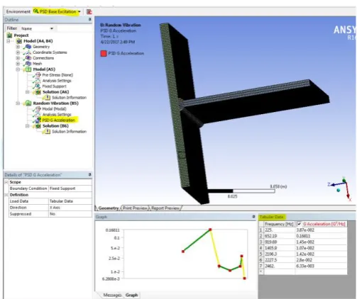
Above shown physical setup requires to be replicated into a Labview circuit, which should be able to measure the force and accelerations inputs exist at the source or the area of evaluation. Hammer is the instrument can be seen in the above figure. does have Piezoelectric Transducer at the tip of impact area; other end of the Hammer is connected to the cDAQ via. Cable. Similarly accelerometer is placed at the area-of-consideration, to acquire the acceleration signal. Both these signal are collected by DAQ, but to understand in the system we need to connect them at particular ports, in this case they are named as a0, a1, a2,a3 (present DAQ is 4 port system). All acquired signals. Once the circuit is built to extract the input signals now next step is to convert this time domain signals into the desired format. Working environment of the project is random in nature, as discussed in the chapter 3, processed signals has to be in frequency domain and known as power spectral density. Below circuit is the basic inclusion of the VI’s into the circuit, and consequent graphs indicate the acceleration and PSD format

Fig - 2:View of corrected PSD circuit

Fig - 3: Output graph of time domain acceleration & frequency domain PSD

Fig - 4: View of PSD input to find out Stresses.

Fig - 5: View of Response PSD at critical zone

© 2017, IRJET | Impact Factor value: 5.181 | ISO 9001:2008 Certified Journal

| Page 3488

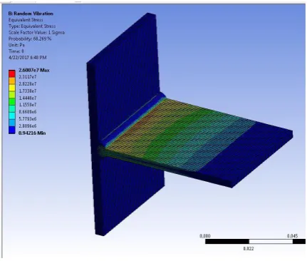
Here in Fig.-7, contour of stress is plotted at left side of the model and is indicated by the different colors according to the stresses generated in the component which has undergone the random loading. From the figure it is evident that a 1σ stress of 26.007MPa is generated at the weld bead location indicated by the red zone, blue color indicates the minimum load experienced by the component and is obviously at the fixed support due to constraints and source of frequency generation.

Fig - 7: View of 1σ stresses at the weld location

5. FATIGUE LIFE CALCULATIONS: “Miner Rule”

The approximate number of stress cycles N1 required to produce a fatigue failure in the

beam for the 1σ, 2σ and 3σ stresses can be obtained from the following equation:

N1=N2 [S1 / S2]b’

N2 = 1000 (S1000 reference point)

S2 = Stress to fail at S1000 reference point) =279.32 MPa S1 = = 1 σ stress from random vibration analysis For load case 1: 26.007 Mpa

b' = slope of fatigue line = 1/-b

Sf = Endurance strength at 103 cycles

Se = Endurance strength at 106 cycles and is given by for

material endurance of Se*:

Se = Ka*Kb*Kc*Ke*Se*

Ka = Surface finish factor = 271*



Kb =Size factor

Kc =Load factor= 1.4335*



Ke =Stress concentration factor

Slope (b) of the SN curve I given by:

© 2017, IRJET | Impact Factor value: 5.181 | ISO 9001:2008 Certified Journal

| Page 3489

Damage accumulated for the load case 1

n1 = 1σ n1 = (180cyc/sec) x (4 hr) x (60 x 60 sec/hr) x (0.683)

= 1.77 x 106 _cycles

n2 = 2σ n1 = (180cyc/sec) x (4 hr) x (60 x 60 sec/hr) x (0.271)

= 7.02 x 105 _cycles

n3 = 3σ n1 = (180cyc/sec) x (4 hr) x (60 x 60 sec/hr) x (0.0433)

= 1.12 x 105 _cycles

1σ N1 =1000 [279.32 / 26.007]5.30

= 2.94x 108_cycles

2σ N1 =1000 [279.32 / 52.014]5.30

= 7.46 x 106 _cycles

3σ N1=1000 [279.32 / 78.021]5.30

=8.68x 105 _cycles

Damage accumulation for 1σ loading Di= ni/Ni

D1=1.77E6_/2.94E8

D1= 0.006

Damage accumulation for 2σ loading

D2=7.02E5_/7.46E6

D2= 0.0942

Damage accumulation for 3σ loading

D3=1.12E6_/8.68E5

D3= 0.1292

Total damage accumulation for all load case is given by D = D1+D2+D3

= 0.006+0.0942 +0.1292 = 0.2294

D = 0.2294< 1

Total damage accumulated is 0.2294, which is less than 1. Therefore a crack will not get initiated in the weld component for the given loading condition. Therefore the service life of structure is found out by taking the damage accumulation of 0.2294.

6. RESULT & DISCUSSION

In this section discussion should be held in three main stages:

First one is to select the right combination of the geometrical variables, this is done with the help of Taguchi method; below are 9 combinations selected and are processed further to carry out the analysis in the random environment. Here Experiment naming is done to include the variable value selected in the respective experiment.

Load case Geometry feature σ1 MPa σ2 Mpa σ3 Mpa 1 T Joint_90_B1.5_H4_W5 26.007 52.014 78.021 2 T Joint_90_B1.25_H3.5_W4 25.528 51.056 76.584 3 T Joint_90_B1_H3_W3.5 27.724 55.448 83.172 4 T Joint_100_B1.5_H3_W4 28.422 56.844 85.266 5 T Joint_100_B1.25_H4_W3.5 28.084 56.168 84.252 6 T Joint_100_B1_H3.5_W5 24.804 49.608 74.412 7 T Joint_105_B1.5_H3.5_W3.5 26.868 53.736 80.604 8 T Joint_105_B1.25_H3_W5 26.399 52.798 79.197 9 T Joint_105_B1_H4_W4 27.834 55.668 83.502

For the selected geometry, all results are evaluated in the random environment, here the base of the T-joint is excited at the fixed end with PSD values as an input; all stress results are taken for the common input excitation. Equivalent stresses are plotted against the entire geometry, below table indicates the maximum stresses each geometry experiences. From the available results maximum stresses are observed at the weld bead location. Further 4th load case with reinforcement angle 100º, edge preparation of 1.5mm, weld bead height as 3mm and width from the centre as 4mm experiences maximum stresses amongst the selected samples. At the same time, 6th load case experiences least stress amongst all samples. All results are available in the appendix section. As we are predicting the results based on the probabilistic approach 1, 2, 3 values are calculated in the below table. Below image demonstrate the max and min stress condition stresses.

Load case Geometry feature σ1 MPa σ2 Mpa σ3 Mpa

1 T Joint_90_B1.5_H4_W5 26.007 52.014 78.021

2 T Joint_90_B1.25_H3.5_W4 25.528 51.056 76.584

3 T Joint_90_B1_H3_W3.5 27.724 55.448 83.172

4 T Joint_100_B1.5_H3_W4 28.422 56.844 85.266

5 T Joint_100_B1.25_H4_W3.5 28.084 56.168 84.252

6 T Joint_100_B1_H3.5_W5 24.804 49.608 74.412

7 T Joint_105_B1.5_H3.5_W3.5 26.868 53.736 80.604

8 T Joint_105_B1.25_H3_W5 26.399 52.798 79.197

9 T Joint_105_B1_H4_W4 27.834 55.668 83.502

© 2017, IRJET | Impact Factor value: 5.181 | ISO 9001:2008 Certified Journal

| Page 3490

for 12Hrs of duty contains least damaging factor of 0.178 and this is the cumulative damages gathered by each of the excitation stress phases, from the calculation conducted in the previous chapter indicates 3σ stresses contribute most damages out of all excitation phases. Damaging factor thus helps in calculating the remaining life of the component. Here in the below table, remaining life is calculated considering samples are excited with all σ stresses and for equal duration of time. This is the adverse condition under consideration. In probabilistic approach, 1 σ stress should excite for 68.3% of total duration, 2 σ stress for 27.1% of entire duration and 4.33% time for 3 σ stress excitation. From the calculation maximum remaining life is for 6th sample and can last for another 55 Hrs and 23min. Please note that all σ stresses are considered for equal amount of excitation time. Load case n1 Cycles n2 Cycles n3 Cycles N1 Cycles N2 Cycles N3 Cycles Damage Factor after 12 Hrs (D) Remaining life In Hrs

1 1.77E+06 7.02E+05 1.12E+05 2.94E+08 7.46E+06 8.68E+05 0.229 40.30 2 1.77E+06 7.02E+05 1.12E+05 3.25E+08 8.23E+06 9.58E+05 0.208 45.72 3 1.77E+06 7.02E+05 1.12E+05 2.10E+08 5.31E+06 6.19E+05 0.322 25.26 4 1.77E+06 7.02E+05 1.12E+05 1.84E+08 4.66E+06 5.42E+05 0.367 20.66 5 1.77E+06 7.02E+05 1.12E+05 1.96E+08 4.96E+06 5.78E+05 0.345 22.80 6 1.77E+06 7.02E+05 1.12E+05 3.78E+08 9.59E+06 1.12E+06 0.178 55.23 7 1.77E+06 7.02E+05 1.12E+05 2.48E+08 6.27E+06 7.31E+05 0.273 32.00 8 1.77E+06 7.02E+05 1.12E+05 2.72E+08 6.89E+06 8.02E+05 0.248 36.31 9 1.77E+06 7.02E+05 1.12E+05 2.05E+08 5.20E+06 6.06E+05 0.329 24.49

IRJET sample template format ,Conclusion content comes here. Conclusion content comes here Conclusion content comes here Conclusion content comes here Conclusion content comes here Conclusion content comes here Conclusion content comes here Conclusion content comes here Conclusion content comes here Conclusion content comes here Conclusion content comes here Conclusion content comes here Conclusion content comes here . Conclusion content comes here

6. CONCLUSION

1. Stress analysis of the welded joint is carried out and maximum 1σ stresses are identified at the weld bead location of the T joint. The joint has been analyzed under the action of frequency domain function of random excitation called as power spectral density and is measured in terms of G2/Hz and this is due vibrations generated from the engine source. Maximum 1σ stresses of 28.422 MPa are observed near the welded geometry and falls near the critical area of welded structure.

2. Taguchi approach is applied to the geometrical variables, tis process of DOE could help us in reducing the efforts to carry out all procedural experiments for around 81 samples. This method helps in reducing the sample straight away by 72 number to 9 sample for consideration.

3. Initiation of the fatigue crack is normally initiated at the location of maximum σ stress in the welded structure. Fatigue calculations are calculated for all three σ values and for equal duration of time, this is the adverse condition under consideration and found that the 6th sample could last

long compared to the other models at the same time weld geometry in the 4th sample experiences least fatigue life amongst the all samples. This entire procedure helps us to understand the random behavior of the system, predict the damaging state of the component, areas affected by the loading and remaining life in the adverse situation.

REFERENCES

[1] Seung-Ho Han, Dae-Gyun An, Seong-Jong Kwak and Ki-Weon Kang “Vibration fatigue analysis for multi-point spot-welded joints based on frequency response changes due to fatigue damage accumulation” International Journal of Fatigue 48 (2013) 170–177.

[2] Wang Chengcheng, Li Chuanri, Xu Fei, and Guo Ying “Research on the Predict Method of Random Vibration Cumulative Fatigue Damage Life Based on the Finite Element Analysis” International Journal of Mechanical, Aerospace, Industrial, Mechatronic and Manufacturing Engineering Vol:6, No:12, 2012

[3] Karteek Navuri, Eswara Kumar A., Beulah Mani P. and B. Satya Krishna “Random Vibration Analysis Of Mechanical Hardware Of Flight Data Recorder” ARPN Journal of Engineering and Applied Sciences, VOL. 11, NO. 18, September 2016

[4] Ahmet H. Ertas and Fazıl O. Sonmez “Design optimization of spot-welded plates for maximum fatigue life” Finite Elements in Analysis and Design 47 (2011) 413–423.

[5] S. M. Nacy, N. K. Alsahib, F. F. Mustafa “Vibration Analysis of Plates With Spot Welded Stiffeners” Jordan Journal of Mechanical and Industrial Engineering, Volume 3, Number 4, December 2009, Pages 272 – 279.

[6] Scot I. McNeill “Implementing the Fatigue Damage Spectrum and Fatigue Damage Equivalent Vibration Testing” 79th Shock and Vibration Symposium, October 2008, Orlando Florido.

[7] K. Sivasakthivel, K. Janarthanan and R .Rajkumar “Optimization of Welding Parameter in MIG Welding by Taguchi Method” International Journal of Advanced Research in Mechanical Engineering & Technology (IJARMET), Vol. 1, Issue 1 (Apr. - Jun. 2015).

[8] M. Bhusnar and S.S. Sarawade “ Modal Analysis of Rectangular plate with lap joints to find natural frequencies and mode shapes” IOSR Journal of Mechanical & Civil Engineering, 5th National Conference RDME March, 2016, PP 06-14.