http://dx.doi.org/10.4236/ojs.2016.64056
How to cite this paper: Zeng, T. and Hill, R.C. (2016) Shrinkage Estimation in the Random Parameters Logit Model. Open Journal of Statistics, 6, 667-674. http://dx.doi.org/10.4236/ojs.2016.64056
Shrinkage Estimation in the Random
Parameters Logit Model
Tong Zeng
1, R. Carter Hill
21Department of Applied Business Sciences and Economics, University of La Verne, La Verne, CA, USA 2Department of Economics, Louisiana State University, Baton Rouge, LA, USA
Received 10 May 2016; accepted 20 August 2016; published 23 August 2016
Copyright © 2016 by authors and Scientific Research Publishing Inc.
This work is licensed under the Creative Commons Attribution International License (CC BY). http://creativecommons.org/licenses/by/4.0/
Abstract
In this paper, we explore the properties of a positive-part Stein-like estimator which is a stochas-tically weighted convex combination of a fully correlated parameter model estimator and uncor-related parameter model estimator in the Random Parameters Logit (RPL) model. The results of our Monte Carlo experiments show that the positive-part Stein-like estimator provides smaller MSE than the pretest estimator in the fully correlated RPL model. Both of them outperform the fully correlated RPL model estimator and provide more accurate information on the share of pop-ulation putting a positive or negative value on the alternative attributes than the fully correlated RPL model estimates. The Monte Carlo mean estimates of direct elasticity with pretest and posi-tive-part Stein-like estimators are closer to the true value and have smaller standard errors than those with fully correlated RPL model estimator.
Keywords
Pretest Estimator, Stein-Rule Estimator, Positive-Part Stein-Like Estimator, Likelihood Ratio Test, Random Parameters Logit Model
1. Introduction
668
The key feature of the RPL model is that response parameters can vary randomly, following a chosen distribution, across the population from which samples are drawn. The random coefficients capture individual heterogeneity and the model does not suffer from the independence of irrelevant alternatives assumption. The random coefficients can be correlated in the RPL model as generally expected in reality, because the unobservable preference of each individual is used to evaluate the attributes of all alternatives in each choice situation. Estimation is by maximum simulated likelihood (MSL), which is described by [1].
In this paper we explore a problem that can exist in any correlated random parameters model. Let yn, 1, ,
n= N be an observable outcome variable from a density f y
(
n|xn,βn)
, where xn is a vector of Kexplanatory variables and βn are random parameters with mean β and covariance matrix Σ. Using MSL we estimate the population parameters β and Σ. Allowing the random parameters to be correlated introduces potentially many new parameters, K K
(
−1 2)
covariance terms, that are difficult to estimate.Most applied researchers will test the significance of the covariance parameters before deciding to rely on the fully correlated random parameter model instead the model in which the parameters are random but uncorrelated, so that Σ is diagonal. We explore whether a pretesting strategy improves postestimation inference. We also explore the use of a Stein-like shrinkage estimator as an alternative to pretesting. This estimator shrinks the estimates from the fully correlated parameter model towards the estimates of the uncorrelated random parameter model. In numerical experiments using the RPL model we find that both the pretest estimator and shrinkage estimators have improved mean squared error (MSE) relative to the MSL estimator of the fully correlated parameter model. Last, we analyze the share of the population putting a positive or negative value on the alternative attributes, and the Monte Carlo mean estimates of direct elasticity with fully correlated RPL model estimates and pretest and shrinkage estimates. Based on our Monte Carlo experiment results, pretest and shrinkage estimates provide more accurate estimates on both of them than the fully correlated RPL model estimates.
2. The Random Parameters Logit Model
The RPL model is described in [2]. Consider individual n facing M alternatives. The random utility associated with alternative i is Uni =βn′xni+εni, where xni are K observed explanatory variables for alternative i, εni is an iid type I extreme value error which is independent of βn and xni. The random coefficients βn can be regarded as being composed of a mean β and deviations βn. The RPL model decomposes the unobserved part of the utility into the extreme value term εni and the random part β ′nxni. Conditional on βn the pro- bability that individual n chooses alternative i is of the usual logistic form,
( )
e n nix e n nixni n i
L β = β′
∑
β′ . Assumethat βn is multivariate normal1 with mean vector β′ =
(
β1,,βk)
and covariance matrix Σ with elementsjk
σ . Denoting the MVN density f
(
β θ|)
, where θ contains the unknown mean and covariance parameters, the probability that individual n chooses alternative i is( ) (
|)
dni ni
P =
∫
L β f β θ β (1)For estimation purposes we use Cholesky’s decomposition and write Σ =AA′, where A is lower triangular. The parameter means βk and elements of A are the objects of estimation. The parameters of the fully cor- related RPL model (FCRPLM), are
(
1, , , 11, , , 21, , , 1)
f k a akk a ak k
θ = β β − (2)
where akk are diagonal elements of A and ajk, j<k, are below the diagonal. If the random coefficients in the RPL model are uncorrelated, denoted UCRPLM, then θ is
(
1, , , 11, ,)
u k a akk
θ = β β (3)
where 2 2
k akk
σ = .
3. Stein-Like Shrinkage Estimation
Stein-rule estimators follow the work of [3] and [4] and combine sample information with non-sample infor-
669
mation in a way that improve the precision of the estimation process and the quality of subsequent predictions. The Stein-rule estimator is a weighted average of the restricted and unrestricted estimators, the weight being a function of the magnitude of the test statistic used to test the restrictions.
Following is the Stein-rule estimator which dominates the maximum likelihood estimator (MLE) in linear regression under weighted quadratic loss with weight matrix W, y=X
β
+e, where y is a(
T×1)
random vector, X is a(
T×K)
matrix of rank K≤T and e is a(
T×1)
vector of random disturbances distributed as(
2)
0,
N σ I . If R
β
=r represent a set of G≤K independent linear restrictions onβ
, the Stein-rule estimator that combines sample and non-sample information is:( )
(
)
(
)
(
)
(
)
* * *
1 1
ˆ, 1 ˆ
ˆ ˆ
as s
r R R X X R r R
δ β β β β
β − − β
= − − + ′ − ′ ′ − (4)
where
β
* is the restricted estimator, obtained by minimizing the sum of squared errors subject to the set of re-strictions,
(
)
(
)
(
)
1
1 1
* ˆ ˆ
X X R R X X R r R
β β ′ − ′ ′ − ′− β
= + − . Here s=
(
y−xb) (
′ y−xb)
with b=(
X X′)
−1X Y′ .Sufficient conditions for minimaxity, meaning that the estimator minimizes the maximum risk over the entire parameter space, are G>2 restrictions and the scalar a chosen to lie within the interval
(
0,amax)
:(
)
(
)
(
)
{
1 1 1 1}
2
0 2
2 L
tr R X X R R X X W X X R
a
T K η
−
− − −
′ ′ ′ ′ ′
< < −
− +
(5)
where ηL is the largest characteristic root of the matrix in braces. The estimator *
( )
ˆ,s
δ β can be written as
( )
*(
)
* ** ˆ ˆ * * ˆ *
,s 1 c 1 c c
u u u
δ β = − β β− +β = − β+ β
(6)
where u is the test statistic for the hypothesis R
β
=r, and c*=a T(
−K)
G. If the data support the non- sample information then u will be small and a relatively large weight is placed on the restricted estimatorβ
*. Conversely, if the data do not support the imposed restrictions, u will be large and the unrestricted estimator βˆ is more heavily weighted. When *u<c , the Stein estimator reverses the sign of the estimator βˆ, or the latter is shrunk beyond the hypothesis vector. The problem is resolved by the use of “positive rule” estimator, which preserves the sign of the estimates and dominates the Stein-rule estimator over the entire parameter space.
The positive-part Stein-like estimator
( )
θ+ is a stochastically weighted convex combination of the MLE from an unrestricted model and a restricted MLE subject to J constraints. In our case the unrestricted MLE( )
ˆf
θ comes from the FCRPLM estimates and the restricted MLE from the UCRPLM estimates
( )
θˆu(
)
ˆ 1 ˆ
u f
c c
θ+ = θ + − θ (7)
where c= −1 I(a,∞)
( )(
u 1−a u)
and I(a,∞)( )
u is the indicator function of a test statistic u for the null hy- pothesis that the coefficient covariance matrix is diagonal, or equivalently that the Cholesky elements in Abelow the diagonal are zero. The scalar a controls the amount of shrinkage towards the UCRPLM estimates. The shrinkage estimator θ+ becomes the UCRPLM estimator θu when the test statistic u is less than the value of
a. The larger the value of a, the more weight that is given to the UCRPLM estimates. [5] show that if the number of constraints J>2, then under information weighted quadratic loss the risk of the shrinkage estimator is smaller than the risk of the unrestricted maximum likelihood estimator for any c>0. Common choices for the shrinkage constant are a=2
(
J−2)
and a= −J 2. In our case J=K K(
−1 2)
is the number of cova- riance terms constrained to zero when obtaining the UCRPLM estimates.With test statistic u, the pretest estimator θ* is:
* if if u f u c u c α α θ θ θ ≤
= >
where cα is the critical value of chi-square distribution with J degrees of freedom and significance level
α
. With the given of degrees of freedom, the critical value cα is determined by the level of test significanceα
, which is between 0 and 1. When α=0, pretest estimator θ* becomes UCRPLM estimator θu. When α=1, pretest estimator θ* is FCRPLM estimator θf .4. Monte Carlo Experiments
4.1. Design
In our experiments the number of choice alternatives is M =4 and the number of individuals is N =200. Each individual is assumed to be observed once. The four explanatory variables for each individual and each alternative xni are generated from independent log-normal distributions lnN
(
1, 0.25)
. The coefficients for each individual βn are generated from multivariate normal distribution N( )
β,Σ , with βk =1, k=1,, 4. The variance of each random coefficient is σ =k2 1, k=1,, 4 . The covariance elements σjk=ρ ,, 1, , 4
j k= . The correlation
ρ
takes the values 0, 0.2, 0.4, 0.6, 0.8. The values of xni and βn are held fixed over the NS AM=1000 Monte Carlo samples in each experiment. The choice probability for each individual is generated with the logit-smoothed accept-reject simulator suggested by [6].Our simulation and RPL model estimation were carried out in NLOGIT 5.0. Based on our Monte Carlo experiment results, [7] and [8], we use 100 Halton draws to simulate choice probabilities during MSL estimation. The positive-part Stein-like and pretest estimators were calculated based on the likelihood ratio (LR), Lagrange multiplier (LM) and Wald test statistics with 25%, 5% and 1% significance level. Because the empirical percentile values of LR test are closer to the related critical values than those of LM and Wald tests, we only provide the results based on the LR test statistic. Using Monte Carlo experiments to study the RPL model, especially with correlated parameters, is numerically challenging. Key elements that are worth mentioning are 1) for the uncorrelated parameter model conditional logit estimates were used as starting values; 2) for the correlated parameter model the estimates from 1) were used as starting values; 3) samples for which con- vergence was not achieved were discarded, only 0.3% of the results are unconverged in our Monte Carlo experiments.
4.2. Results
To study how the pretest and shrinkage estimators reduce the estimation risk of the FCRPLM estimators, we calculate the MSEs of the estimated parameters mean, variance, covariance with the pretest, shrinkage and FCRPLM estimators respectively. First, we compare the MSE of the fully correlated estimators and those of
UCRPLM estimators, where MSE is the Monte Carlo average of the squared error loss 4
(
)
2 1 ˆk k k= β −β [image:4.595.87.538.621.720.2]∑
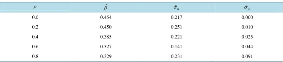
. InTable 1, the MSEs of UCRPLM estimators are all smaller than those of FCRPLM estimators. The risk of the
estimated parameters mean with the FCRPLM is more than twice that of the UCRPLM. The MSEs of the estimated variance with the UCRPLM are about 25% of those with the FCRPLM. With nonzero correlation ρ, the MSEs of estimated covariance parameters based on the FCRPLM are much bigger than those based on the UCRPLM. When the correlation
ρ
=0.2 and 0.4, the ratios of MSEs of estimated covariance elements are relatively smaller compared to the results for higher correlations. This implies that when the specification error is small, the FCRPLM, which is the correct model, has a much larger relative MSE for parameter covariance elements than the UCRPLM.Table 1. The ratios of uncorrelated RPL model estimator MSE to the FCRPLM estimator MSE.
ρ βˆ σˆkk σˆjk
0.0 0.454 0.217 0.000
0.2 0.450 0.251 0.010
0.4 0.385 0.221 0.025
0.6 0.327 0.141 0.044
671
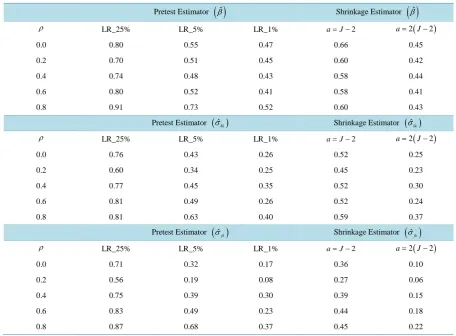
In Table 2, we compare the MSEs of LR based pretest and shrinkage estimators to those of FCRPLM
estimators. All Table 2 ratios are less than one. The pretest and shrinkage estimators all perform better than the FCRPLM estimators. With a smaller level of test significance
α
, the UCRPLM estimator θu is more fre- quently chosen as the pretest estimator and the pretest estimator has smaller MSE. However, compared to the shrinkage estimators, the LR based pretest estimators with α=0.01 have larger MSEs than the shrinkage estimators with the shrinkage constant a=2(
J−2)
, especially for the estimated covariance elements, which have the smallest ratio values.The covariance elements reveal important information about the joint effect of alternative attributes on people' decisions. If two random coefficients are highly positively correlated with each other, it means people are attracted and motivated by both of the related attributes. In our Monte Carlo experiments, the shrinkage estimators with higher shrinkage constant a outperform estimators with less shrinkage and most of the pretest estimators.
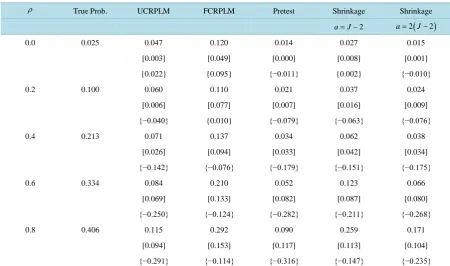
Since one of the advantages of RPL model is providing the information on the share of population that places a positive or negative value on the alternative attributes, we also calculate the joint probability of the first two estimated parameters are less than zero. Table 3 shows the share of population putting a negative value on the attributes. Compared to the results with UCRPLM and FCRPLM estimates, the joint probability with FCRPLM estimates are closer to the true value with larger MSEs, except for the
ρ
=0. From Table 3, the pretest and shrinkage estimates reduce the MSE of the joint probability estimator compared to the FCRPL model estimates. Even though the bias of the joint probability with pretest and shrinkage estimates are higher than UCRPLM and FCRPLM estimates, the difference is small in magnitude. [image:5.595.83.540.386.722.2]To analyze the sensitivity of the RPL model in response to a change in the level of alternative attribute, we calculate the mean estimates of direct elasticity with the true parameters
(
β Σ, β)
, Table 4, and the Monte Carlo mean estimates of direct elasticity based on pretest, positive-part Stein-like estimates and FCRPLM estimates,Table 2. The ratios of LR Based pretest, shrinkage estimator MSE to the FCRPLM estimator MSE.
Pretest Estimator
( )
βˆ Shrinkage Estimator( )
βˆρ LR_25% LR_5% LR_1% a= −J 2 a=2
(
J−2)
0.0 0.80 0.55 0.47 0.66 0.45
0.2 0.70 0.51 0.45 0.60 0.42
0.4 0.74 0.48 0.43 0.58 0.44
0.6 0.80 0.52 0.41 0.58 0.41
0.8 0.91 0.73 0.52 0.60 0.43
Pretest Estimator
( )
σˆkk Shrinkage Estimator( )
σˆkkρ LR_25% LR_5% LR_1% a= −J 2 a=2
(
J−2)
0.0 0.76 0.43 0.26 0.52 0.25
0.2 0.60 0.34 0.25 0.45 0.23
0.4 0.77 0.45 0.35 0.52 0.30
0.6 0.81 0.49 0.26 0.52 0.24
0.8 0.81 0.63 0.40 0.59 0.37
Pretest Estimator
( )
σˆjk Shrinkage Estimator( )
σˆjkρ LR_25% LR_5% LR_1% a= −J 2 a=2
(
J−2)
0.0 0.71 0.32 0.17 0.36 0.10
0.2 0.56 0.19 0.08 0.27 0.06
0.4 0.75 0.39 0.30 0.39 0.15
0.6 0.83 0.49 0.23 0.44 0.18
Table 3. The Share of population putting negative value on the first two attributes of each alternative, P
(
β1<0,β2<0)
.ρ True Prob. UCRPLM FCRPLM Pretest Shrinkage Shrinkage
2
a= −J a=2
(
J−2)
[image:6.595.88.539.408.530.2]0.0 0.025 0.047 0.120 0.014 0.027 0.015
[0.003] [0.049] [0.000] [0.008] [0.001]
{0.022} {0.095} {−0.011} {0.002} {−0.010}
0.2 0.100 0.060 0.110 0.021 0.037 0.024
[0.006] [0.077] [0.007] [0.016] [0.009]
{−0.040} {0.010} {−0.079} {−0.063} {−0.076}
0.4 0.213 0.071 0.137 0.034 0.062 0.038
[0.026] [0.094] [0.033] [0.042] [0.034]
{−0.142} {−0.076} {−0.179} {−0.151} {−0.175}
0.6 0.334 0.084 0.210 0.052 0.123 0.066
[0.069] [0.133] [0.082] [0.087] [0.080]
{−0.250} {−0.124} {−0.282} {−0.211} {−0.268}
0.8 0.406 0.115 0.292 0.090 0.259 0.171
[0.094] [0.153] [0.117] [0.113] [0.104]
{−0.291} {−0.114} {−0.316} {−0.147} {−0.235}
Note: [ ] provides the MSE results, {} provides bias results.
Table 4. The mean estimates of direct elasticity with true parameters
(
β,Σβ)
. True RPL Model Parametersρ
(
P x1, 11)
(
P x2, 21)
(
P x3, 31)
(
P x4, 41)
0.0 2.009 1.960 2.053 2.042
0.2 2.014 1.957 2.052 2.049
0.4 2.020 1.954 2.051 2.057
0.6 2.025 1.951 2.051 2.065
0.8 2.031 1.947 2.051 2.075
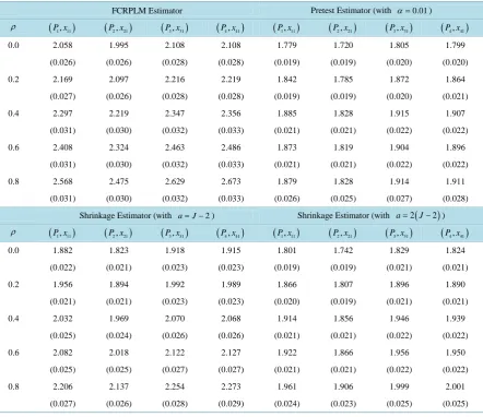
Table 5. Since the pretest estimator with smaller level of test significance has smaller MSE, we use the pretest
estimator with 1% significance level. The first explanatory variable in each alternative xi j, ,1 is chosen to calculate the related mean estimates of direct elasticity.
Comparing the results in Table 4 to Table 5, we find that the results with FCRPLM estimates are all higher than the true value. When the
ρ
>0.2, the results with pretest and shrinkage estimators are closer to the true value than those based on the FCRPLM estimators. The shrinkage estimators with the larger shrinkage constant have smaller bias of the Monte Carlo mean direct elasticity estimates than the pretest estimates and shrinkage estimates with smaller shrinkage constant. At the same time, the shrinkage and pretest estimators have smaller standard error of the Monte Carlo mean direct elasticity estimates than the FCRPLM estimates. Based on our Monte Carlo experiment results, the shrinkage and pretest estimates will give more reliable mean direct elasticity estimates than the FCRPLM estimates, especially with a larger shrinkage constant.5. Conclusion
673
Table 5. The Monte Carlo mean estimates of direct elasticity based on pretest, shrinkage and FCRPLM estimates.
FCRPLM Estimator Pretest Estimator (with α=0.01)
ρ
(
)
1, 11
P x
(
P x2, 21)
(
P x3, 31)
(
P x4, 41)
(
P x1, 11)
(
P x2, 21)
(
P x3, 31)
(
P x4, 41)
0.0 2.058 1.995 2.108 2.108 1.779 1.720 1.805 1.799
(0.026) (0.026) (0.028) (0.028) (0.019) (0.019) (0.020) (0.020)
0.2 2.169 2.097 2.216 2.219 1.842 1.785 1.872 1.864
(0.027) (0.026) (0.028) (0.028) (0.019) (0.019) (0.020) (0.021)
0.4 2.297 2.219 2.347 2.356 1.885 1.828 1.915 1.907
(0.031) (0.030) (0.032) (0.033) (0.021) (0.021) (0.022) (0.022)
0.6 2.408 2.324 2.463 2.486 1.873 1.819 1.904 1.896
(0.031) (0.030) (0.032) (0.033) (0.021) (0.021) (0.022) (0.022)
0.8 2.568 2.475 2.629 2.673 1.879 1.828 1.914 1.911
(0.031) (0.030) (0.032) (0.033) (0.026) (0.025) (0.027) (0.028)
Shrinkage Estimator (with a= −J 2) Shrinkage Estimator (with a=2
(
J−2)
) ρ(
P x1, 11)
(
P x2, 21)
(
P x3, 31)
(
P x4, 41)
(
P x1, 11)
(
P x2, 21)
(
P x3, 31)
(
P x4, 41)
0.0 1.882 1.823 1.918 1.915 1.801 1.742 1.829 1.824
(0.022) (0.021) (0.023) (0.023) (0.019) (0.019) (0.021) (0.021)
0.2 1.956 1.894 1.992 1.989 1.866 1.807 1.896 1.890
(0.021) (0.021) (0.023) (0.023) (0.020) (0.019) (0.021) (0.021)
0.4 2.032 1.969 2.070 2.068 1.914 1.856 1.946 1.939
(0.025) (0.024) (0.026) (0.026) (0.021) (0.021) (0.022) (0.022)
0.6 2.082 2.018 2.122 2.127 1.922 1.866 1.956 1.950
(0.025) (0.025) (0.027) (0.027) (0.021) (0.021) (0.022) (0.022)
0.8 2.206 2.137 2.254 2.273 1.961 1.906 1.999 2.001
(0.027) (0.026) (0.028) (0.029) (0.024) (0.023) (0.025) (0.025)
Note: ( ) provides the standard error results.
FCRPLM estimators. The pretest and positive-part Stein-like estimators both perform better than the FCRPLM estimators. The positive-part Stein-like estimators with higher shrinkage constant a outperform those with a smaller one and the pretest estimators. Shrinkage estimation reduces the risk of the FCRPLM estimators by shrinking the FCRPLM estimates towards the UCRPLM estimates. Providing the information on the share of population putting a negative or positive value on the alternative attributes is one of the advantages of the RPL model. When the random coefficients are correlated to each other, the FCRPLM estimator of this quantity has a smaller bias and slightly larger MSE than the UCRPLM estimator. Based on our Monte Carlo experiments, the pretest and shrinkage estimates can reduce the MSEs of the estimated results of share of the population putting a positive or negative value on alternative attributes as well. The Monte Carlo mean estimates of direct elasticity based on the pretest and shrinkage estimators with a larger shrinkage constant are closer to the true value with smaller standard errors than those based on the FCRPLM estimators.
References
[1] Greene, W.H. (2012) Econometric Analysis. Pearson Education, Inc., NJ.
[2] Train, K.E. (2009)Discrete Choice Methods with Simulation. Cambridge University Press, Cambridge.
http://dx.doi.org/10.1017/CBO9780511805271
[4] Stein, C.M. (1956) Inadmissibility of the Usual Estimator for the Mean of a Multivariate Normal Distribution. Pro-ceedings of the Third Berkeley Symposium on Mathematical Statistics and Probability, 1954-1955, I, 197-206. Univer-sity California Press, Berkeley.
[5] Kim, M. and Hill, R.C. (1995) Shrinkage Estimation in Nonlinear Regression: the Box-Cox Transformation. Journal of Econometrics, 66, 1-33. http://dx.doi.org/10.1016/0304-4076(94)01606-Z
[6] McFadden, D. (1989) A Method of Simulated Moments for Estimation of Discrete Response Models without Numeri-cal Integration. Econometrica, 57, 995-1026. http://dx.doi.org/10.2307/1913621
[7] Bhat, C.R. (2001) Quasi-Random Maximum Simulated Likelihood Estimation of the Mixed Multinomial Logit Model.
Transportation Research Part B, 35, 677-693. http://dx.doi.org/10.1016/S0191-2615(00)00014-X
[8] Zeng, T. (2016)Using Halton Sequences in Random Parameters Logit Models. Journal of Statistical and Econometric Methods, 5, 59-86.
Submit or recommend next manuscript to SCIRP and we will provide best service for you:
Accepting pre-submission inquiries through Email, Facebook, LinkedIn, Twitter, etc. A wide selection of journals (inclusive of 9 subjects, more than 200 journals) Providing 24-hour high-quality service
User-friendly online submission system Fair and swift peer-review system
Efficient typesetting and proofreading procedure
Display of the result of downloads and visits, as well as the number of cited articles Maximum dissemination of your research work