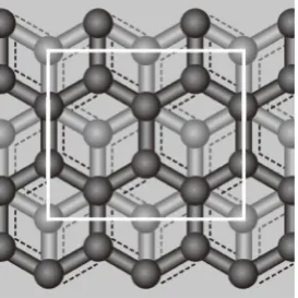
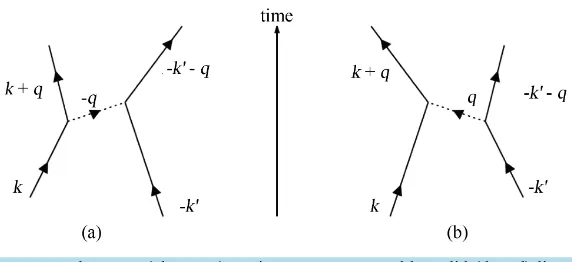
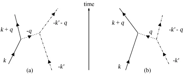
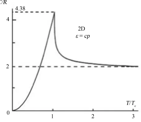
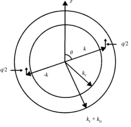
Quantum Statistical Theory of Superconductivity in MgB2

Subsequently, the access level measure, along with land-use and design measures, was employed in three NBR models to explore the importance of including the accessibility

We assayed the micronuclear genotypes of the clones derived from each parent of the noncon- jugant pairs (termed the exconjugant clones) by a testcross to SB210, a hetero-

It addresses the budgetary process cycle and the four main phases: the preparation of a national budget proposal phase, the national budget adoption phase, the

Banking of pluripotent adult stem cells as an unlimited source for red blood cell production: potential applications for al- loimmunized patients and rare blood challenges. Stem

Both the Director of Methodology and the Technical Director spend a large part of their time observing training sessions and matches and again, for the most part, what we see

Solid state fermentation was carried out at optimum growth conditions for maximum xylanase production using wheat bran waste, corn cobs wastes, and pigeon pea pod

The results of our study showed, compared with women without periodontal disease, pre-conception women with moderate/severe periodontal disease had significantly

According to Wagstaff and others, when the concentration curve for health care payments lies completely outside the Lorenz curve of ATP or SES (which in this case is based on