A Theoretical Foundation for the Widely Linear Processing of Quaternion Valued Data

(1)

http://dx.doi.org/10.4236/am.2013.412219

A Theoretical Foundation for the Widely Linear Processing

of Quaternion-Valued Data

Tohru Nitta

National Institute of Advanced Industrial Science and Technology (AIST), Tsukuba, Japan Email: [email protected]

Received June 7, 2013; revised July 7, 2013; accepted July 15, 2013

Copyright © 2013 Tohru Nitta. This is an open access article distributed under the Creative Commons Attribution License, which permits unrestricted use, distribution, and reproduction in any medium, provided the original work is properly cited.

ABSTRACT

In this paper, we will give a theoretical foundation for a quaternion-valued widely linear estimation framework. The estimation error obtained with the quaternion-valued widely linear estimation method is proved to be smaller than that obtained using the usual quaternion-valued linear estimation method.

Keywords: Augmented Statistics; Complex Number; Estimation; Quaternion

1. Introduction

The widely linear (WL) estimation method has been proved mathematically to be effective for estimation prob- lems using complex-valued data. Estimation using WL uses complex conjugate parameters in addition to complex-valued parameters [1]. It has been applied to communications [2,3] and adaptive filters [4], together with so-called augmented complex statistics, a concept introduced by Picinbono et al. Moreover, an extension of the WL method to quaternion-valued case has been pre- sented [5], which fully exploits available statistical information. A quaternion, a four-dimensional number invented by W. R. Hamilton in 1843, is an extension of a complex number. Let H be a four-dimensional vector space over with an ordered basis, denoted by and where is a set of real numbers. Any quarternion

R 1, ,i j

k q

R

H is expressed as where . The three basis elements satisfy the relations

q  a ib jckd

, ,

i j k

, ,

a b c d, R

2 2 2 _1,

i  j k   (1)

, ,

ij  ji k jk  kj i ki  ik j. (2)

Quaternion algebra has been used in fields such as ro- botics, computer vision, neural networks, signal processing, and communications (e.g. [6-8]).

In this paper, we present a theoretical foundation for quaternion-valued WL estimation: it is proved that the estimation error obtained using the quaternion-valued WL estimation method is smaller than that obtained us-

ing the usual quaternion-valued estimation method [9].

2. The WL Model

In this section, the complex-valued WL model and the quaternion-valued WL model are reviewed.

2.1. The Complex-Valued WL Model

Let yC be a scalar complex-valued random variable to be estimated in terms of an observation that is a complex-valued random vector _ N

x C

N

x

where is a set of complex numbers, and is a natural number. That is, is a true value and is an observed value. In complex-valued linear mean square estimation (LMSE), the problem is to find an estimate written as

C

y

ˆ H ,

L

y h x (3) where _h__CN_{, and}_H _{represents the complex conju-}

gation and transposition. Then, the objective of the problem is to find the parameter _h__CN_{that minimizes the}

estimation error E yyˆL 2.

In the meantime, the complex-valued widely linear mean square estimation (WLMSE) problem can be stated as follows: Consider the scalar yˆ defined as

ˆ H H ,

yh xg x (4) where _{g h}, _CN_{, and} def

v a bi is the complex conjugate of v  a bi C

,

. Then, the objective of the problem is to find parameters _{g h}_CN _{that minimize}

(2)

Picinbono et al. gave a theoretical foundation for the complex-valued WLMSE described above: it was proved that the estimation error obtained using the complex- valued WLMSE method is smaller than that obtained using the usual complex-valued LMSE method:

2

ˆ_L ˆ

E yy E yy2 where the equality holds only in exceptional cases [1].

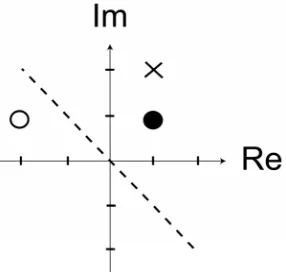
[image:2.595.101.244.573.709.2]

Figures 1 and 2 demonstrate the effectiveness of complex-valued widely linear estimation. Samples of complex-valued random variable x and y are axisymmetric about the broken line: the white circle, the black circle, and the christcross in Figure 1 correspond to the white circle, the black circle, and the christcross in Figure 2, respectively, and the three marks in Figure 1 and the three marks in Figure 2 are all axisymmetric about the broken line. It is therefore difficult to estimate the three samples in Figure 1 by performing rotation, reduction, or expansion of the three samples in Figure 2 about the origin. Nevertheless, inversion of the samples about the real axis, i.e., assuming it as the samples of conjugate complex-valued random variable, allows to be estimated by rotation, reduction, and expansion about the origin. This is an intuitive explanation that the complex-valued widely linear estimation is superior to the conventional linear estimation method.

Figure 1. Three samples of a complex-valued random vari- able x.

Figure 2. Three samples of a complex-valued random vari- able y.

2.2. The Quaternion-Valued WL Model

The quaternion-valued WL model is a natural extension of the complex-valued WL model described in Section 2.1. Let yH be a scalar quaternion-valued random variable to be estimated in terms of an observation that is a quaternion-valued random vector _ N

x H . That is, y is a true value and x is an observed value.

In quaternion-valued linear mean square estimation (LMSE), the problem is to find an estimate written as

ˆ H ,

L

y h x (5) where _h_HN_,

N is a natural number, and H represents the quaternionic conjugation and transposition.

The quaternion-valued widely linear mean square estimation (WLMSE) problem can be stated as follows: Consider the scalar yˆ defined as

ˆ H H ,

yh xg x (6) where _{g h}, __HN

bi cj dk

, N is a natural number, H represents the quaternionic conjugation and transposition, and _def

v   a bi cj dk

is the quaternionic conjugate of v   a H. Then, the objective of the problem is to find parameters _{g h}, __HN _{that minimize}

2

ˆ E yy .

Took and Mandic derived an augmented quaternion least mean squares (AQLMS) algorithm for quaternion valued adaptive filters based on the quaternion-valued WL model, and confirmed its effectiveness via computer simulations [5]. Actually, the experimental results on the Lorenz attractor, real-world wind forecasting, and data fusion via quaternion spaces support the approach. Con- sequently, computer simulations proved that the quarternion-valued WL estimation method is superior to the usual quaternion-valued linear estimation method.

Moreover, the three perpendicular quaternion involutions can be introduced into the quaternion-valued WLMSE, which are given by

,

i

q  iqi  a ib jckd (7)

,

j

q  jqj  a ib jckd (8)

,

k

q  kqk  a ib jckd (9) where q  a ib jckdH [10-12]. The quarternion-valued WLMSE using (6) is an initial insight. However, in order to achieve the complete description of the second order statistics in H,

ˆ y

we need to consider the involutions ((7)-(9)). Actually, the quaternion-valued widely linear mean square estimation (WLMSE) problem using the involutions has been formulated as follows [12]: Consider the scalar defined as

ˆ H H i H j H k,

yh xg x u x v x (10) where , , , _ N

(3)

lem is to find parameters , , , _ N

g h u v H that minimize

2

ˆ E yy .

However, no theoretical proof for the superiority of the quaternion-valued WL estimation method on estimation errors has been given to date, as it has been for the complex-valued WL estimation method. In the complex- valued setting, Picinbono et al. proved that the estimation error obtained with the complex-valued WLMSE is smaller than the error obtained using the complex-valued LMSE [1].

3. A Theoretical Foundation of the

Quaternion-Valued WL Model

In this section, we show the superiority of the quarternion-valued WLMSE method. The main result is as follows: the estimation error obtained using the quarternion- valued WL estimation method based on (6) is smaller than that obtained using the usual quarternion-valued linear estimation method, except in rare cases. The result is obtainable in the same manner described by [1]. How- ever, the noncommutativity of the quaternion products must be considered during the analysis (xyyx for any

,

x yH). Define

 





def

, .

H H

X  Z  h x  g x  g hHN



Therein, X is a set of scalar quaternion-valued random variables that constitutes a linear space, and which be- comes a Hilbert subspace of the one-dimensional quarternion-valued Hilbert space Y 



z

 

 H with the

scalar product z, defE z_ _



z,X



. Then, for a

true value yY, an observed value  N

x H , and the

estimate yˆX , the following equations hold:



yyˆ



x, (12)



yyˆ



x, (13) where means that all the components of are orthogonal to u with the scalar product

uv v

,  



, N



uH vH . From (12) and (13), we obtain

ˆ ,

E_xy_E_xy_

s

(14)

ˆ .

E_x y _E_x y _ (15)

Consequently, from (6), (14), (15), the following equations hold (see the appendices for the detail of the derivation):

1 C r,

 h g (16)

2 ,

H

C h  g  (17) where ₁def_E H,

  xx  def

T

2 E ,



 

  x x 

def

T _,

C Exx _ def

,

r  Exy

 

def

. s E yx



1 H

s C

 _ _ _



1 1

r C 

Equations (16) and (17) yield





1

2 C 1C



 



1 2



H

C C



1



1

1 ,

H

r 

 

g (18)

2s

 _{  } 

 

h  

1 1

(19)

where we assume that  1 and 2







1



1

2 1

H

C C 

  

exist (see the appendices for the detail of the derivation). Then, the estimation error WL is calculated from (6),

(16), and (17) as follows:





def

WL

2 _ˆ2 2 H T _.

E y y E y r s

    h g (20)

The estimation error L in the quaternion-valued

LMSE can be obtained using (5) as shown below.

def

₂ 2 2 ₁

1

ˆ H

L E y yL E y r r



     . (21) Then, from (16) and (18), (20), (21), the quantity _2

can be expressed as







 

2 1

1

1 1

2 1 1 ,

H H

L WL

H H

s C r

C C s C r

  



  

    

    

def

2 2

 

 



C

(22)

which is the difference between the estimation error of the quaternion-valued LMSE and that of the quarternion-valued WLMSE. Equation (22) is nonnegative because the matrix is positive-semidefinite (see the appendices for the proof). Furthermore, (22) is equal to zero only when one of the following conditions holds:

1

2 1

H

C 

  

1

1 ,

H

sC r0 (23) ˆ .

y y (24) Equation (23) is an exceptional case, and (24) means that the true value y can be estimated with probability of one, which is a rare case.

4. Discussions

In the previous section, a theoretical foundation of the quaternion-valued WL model based on (6) is given, which guarantees the superiority of the quaternion-valued WLMSE method. It is difficult to analyze the quaternion-value WLMSE method using (7)-(9) which contains all the necessary second order statistical information because the process of the analysis is very complicated due to the three involutions if we adopt the way of proof used in [1]. To solve the problem, another approach would be needed.

5. Conclusion

(4)

ternion-valued WL estimation method. It was proved that the estimation error obtained using the quaternion-valued WL estimation method is smaller than that obtained using the usual quaternion-valued linear estimation method, except in rare cases. In our future studies, we will pro- ceed with analyses of the WL estimation based on the Clifford algebra [13].

6. Acknowledgements

The author extends special thanks to Prof. B. Picinbono, the Laboratoire des Signaux et Systèmes, Supélec, Gifsur Yvette, France for help in resolving several questions, and the anonymous reviewers for valuable comments.

REFERENCES

[1] B. Picinbono and P. Chevalier, “Widely Linear Estima- tion with Complex Data,” IEEE Transactions on Signal Processing, Vol. 43, No. 8, 1995, pp. 2030-2033. http://dx.doi.org/10.1109/78.403373

[2] H. Gerstacker, R. Schober and A. Lampe, “Receivers with Widely Linear Processing for Frequency-Selective Channels,” IEEE Transactions on Communications, Vol. 51, No. 9, 2003, pp. 1512-1523.

http://dx.doi.org/10.1109/TCOMM.2003.816992

[3] R. Schober, W. H. Gerstacker and L. H.-J. Lampe, “Data- Aided and Blind Stochastic Gradient Algorithms for Widely Linear MMSE MAI Suppression for DS-CDMA,” IEEE Transactions on Signal Processing, Vol. 52, No. 3, 2004, pp. 746-756.

http://dx.doi.org/10.1109/TSP.2003.822359

[4] D. P. Mandic and V. S. L. Goh, “Complex Valued Non- linear Adaptive Filters: Noncircularity, Widely Linear and Neural Models,” John Wiley and Sons Ltd., Hobo- ken, 2009. http://dx.doi.org/10.1002/9780470742624 [5] C. C. Took and D. P. Mandic, “The Quaternion LMS

Algorithm for Adaptive Filtering of Hypercomplex Proc- esses,” IEEE Transactions on Signal Processing, Vol. 57,

No. 4, 2009, pp. 1316-1327.

[6] T. Nitta, “A Quaternary Version of the Back-Propagation Algorithm,” Proceedings of the IEEE International Con- ference on Neural Networks (ICNN’95), Perth, 27 No- vember-1 December, 1995, pp. 2753-2756.

[7] P. Arena, L. Fortuna, G. Muscato and M. G. Xibilia, “Neural Networks in Multidimensional Domains,” Sprin- ger, London, 1998.

[8] T. Isokawa, N. Matsui and H. Nishimura, “Quaternionic Neural Networks: Fundamental Properties and Applica- tions,” In: T. Nitta, Ed., Complex-Valued Neural Net- works: Utilizing High-Dimensional Parameters, Infor- mation Science Reference (IGI Global), Hershey, New York, 2009, pp. 411-439.

http://dx.doi.org/10.4018/978-1-60566-214-5.ch016 [9] T. Nitta, “Widely Linear Processing of Hypercomplex

Signals,” In: B.-L. Lu, L. Zhang and J. Kwok, Eds., Neu- ral Information Processing, Lecture Notes in Computer Science, Springer, Berlin, Heidelberg, 2011, pp. 519-525. [10] C. C. Took and D. P. Mandic, “A Quaternion Widely

Linear Adaptive Filter,” IEEE Transactions on Signal Processing, Vol. 58, No. 8, 2010, pp. 4427-4431.

[11] J. Via, D. Ramirez and I. Santamaria, “Properness and Widely Linear Processing of Quaternion Random Vec- tors,” IEEE Transactions on Information Theory, Vol. 56, No. 7, 2010, pp. 3502-3515.

http://dx.doi.org/10.1109/TIT.2010.2048440

[12] D. P. Mandic, C. Jahanchahi and C. C. Took, “A Quarter- nion Gradient Operator and its Applications,” IEEE Sig- nal Processing Letters, Vol. 18, No. 1, 2011, pp. 47-50. http://dx.doi.org/10.1109/LSP.2010.2091126

(5)

Appendices

Proof of Equations (16) and (17):



ˆ







0 from Equation 12

ˆ .

E y y E y E y

      _  _      _ _ _ _ x x x







  (25)

So, we obtain

ˆ .

E_xy_E_xy _ (26)

Similarly, from Equation (13) we obtain ˆ .

E_x y _E_x y _ (27) Here,







 

  



T

ˆ from Equation 6

.

H H

H

y  

 _ 

 

h x g x

x h x g

(28)

Note that due to the non-

commutativity of the quaternion products. Thus, from Equations (26) and (28),

T _,

H _ 

x h h x x gT g xT

 

T T T _, H H H

E y E E

E E E E  _ _ _               _ _ _ _      _ _  _ _

x x x h x x g

xx h xx g

(29)

which means that Equation (16) holds.

It also follows from Equations (27) and (28),

 

T T T 2 2 . H H H H

E y E E

E E E C                        _ _  _ _    _ _       

x x x h x x

x x h x x g

xx h g

h g   g  (30)

The left hand side of Equation (30) is given as:

 



 



.

E_x y  _ E_ yx _ E yx  s (31)

Equations (30) and (31) complete the proof of Equa- tion (17). ■

Proof of Equations (18) and (19):

From Equation (16), we obtain





1

1 r C .

   h g



h C (32)

Equations (17) and (34) lead Equation (18). And also, from Equation (17), we obtain



1

2 .

H

Cg C  sC (33)

Equations (16) and (33) lead Equation (19). ■

Proof that the matrix is positive- semidefinite: 1 2 1 H C    

Consider the following problem. Let _ N

x H and

N



y H be two random vectors such that

 

E x E y 0. The problem is to estimate linearly y in terms of x, which means to find the N-dimensional quaternion valued matrix M such that yˆMx is the best linear mean square (LMS) estimation of in terms of . The solution is given by the orthogonality principle saying that

y

x

ˆ  

y y y is orthogonal to the observation x or



ˆ



H . That is,

E_ yy x _0

yx M xx

  

def

H xx E

where def H and

E 

  _yx yx 

 

  xx . Assuming that _xx1 exists, the solution is obviously

1_. yx xx

M   

def

(34)

Here, the matrix _ is positive- semidefinite because for any

H

E

  _ yy 

N



u H such that u0,

2

0

H H

E

 

u _u y u  . Using the definition y y yˆ and Equation (34) yield by simple algebra

1

yy yx xx x



y

      _ (35)

where def H

yy E 

  yy  and . def

H

xy E 

  xy 



Suppose now that yx . This yields   _yy ₂,

H

yx C

  , 1 1

xx

1

 

   and . Thus we obtain from Equation (35) xy

C

 

1 2 CH 1C.