RЀNYI ENTROPY FOR MIXTURE MODEL OF ULTIVARIATE SKEW NORMAL CAUCHY DISTRIBUTIONS

(1)

3574

MODIFIED APPROACH FOR SOLVING RANDOM

ORDINARY DIFFERENTIAL EQUATIONS

1_{ALI A. ABDULSAHIB,}2_{FADHEL S. FADHEL AND}3_{SALAH H. ABID}

1,3_{Department of Mathematics, College of Education, Al-Mustansiriyah University, Baghdad, Iraq}

2_{Department of Mathematics and Computer Applications, College of Science, Al-Nahrain University,} Baghdad, Iraq

E-mail: 1_{[email protected],}2_{[email protected],} 3_{[email protected]}

ABSTRACT

This paper deals with the derivation of a modified approach for solving initial value problems of the n-th order random ordinary differential equations by means of using the variational iteration method and numerical integration methods. In addition, the convergence of the obtained sequence of approximate solutions to the exact solution has been proved. Also, some illustrative examples are presented as a numerical simulation in order to illustrate the accuracy and applicability of the proposed approach.

Keywords: Random Ordinary Differential Equations, Variational Iteration Method, Numerical Integration

Method, Trapezoidal Rule.

1. INTRODUCTION

Random ordinary differential equations (RODEs) are considered to be an ordinary differential equation (ODE) that includes a stochastic process in their vector field. They seem to have a shadow existence as a shadow of stochastic ordinary differential equations (SODEs) with Itô process, which have so many well-known real life applications. In particular, RODEs play a fundamental role in the theory of random dynamical systems and/or modern control theory, [1,2].

Random ordinary differential equations, unlike SODEs, can be analyzed path wise with deterministic calculus, which require further analytical treatments beyond that of classical theory of ODEs, [3]. Specifically, since the deriving process in a RODE has at most Hölder continuous sample path, then the solution as a sample path is continuously differentiable, but the sample path of the derivative is no more than Hölder continuous in time, [4]. The obtained vector field resulting after introducing the deriving stochastic process is at most of Hölder continuous in time, and no matter how smooth the vector field is in its original variables. Therefore, the RODE solutions do not have sufficient smoothness and after that to have in the usual sense Taylor expansions.

In older mathematical physics and engineering literatures, simple kinds of RODEs are investigated with the vector field being chosen depending on random variables rather than depending on stochastic processes. Such RODEs are still of great importance in the uncertainty qualification community, which are a special case of stochastic models and considered by Xiaoying Han and Peter E. Kloden, and will not be treated separately, [4]. So many applications of real life problems in biology, physics and engineering involving rate of change that depends on the interaction of the basic particles, changes, populations, etc. in addition to the stochastic or random effects, which will produce models that formulated as RODEs, such that the solution of the differential equation which are measured experimentally are in fact not predicted, [3].

(2)

3575 R. et al. in 2011 [12, 13] used the Adomian decomposition method and variational iteration method (VIM) to solve certain types of second order RODEs. In 2013, Farnaoosh R. et al. [14] present the numerical solution of ODEs with Gaussian random coefficients and time-varying using Euler-Maruyama and Milston methods. Runge-Kutta method had been used by Nouri K. and Ranjbar H. in 2015 [15] to find the numerical solution of initial value problems of RODEs. The mean and variance of the approximate solutions of the second-order RODEs using homotopy analysis method have been proposed by Khudair A. R. et al. in 2016 [16]. Tchier F. et al. in 2017 [17] study a family of RDEs with boundary conditions using random fixed point theorem.

Consequently to the above discussion, closed form solution of RODEs seems to be very difficult to evaluate and hence an accurate and reliable numerical and/or approximate methods are necessary to solve such type of problems. Thus, in this paper, one of the well-known approximate-numerical methods will be used to solve RODEs by introducing a modified approach which consists of combining the VIM and numerical integration methods to approximate the integral of the correction functional. This approach will treat the difficulties that arise upon using the Wiener process related to the integral operator appeared in the VIM.

2. PRELIMINARIES

In this section and for completeness purpose, some fundamental and basic concepts related to the present work of this paper are presented, where more elementary concepts will not be given. As a notation, we will consider (,F,P) as the probability space, which comprises the sample space , a -algebra F of subsets of  (called events) and a probability measure P on F.

We start with the following basic definitions:

Definition 1 [1, 8]:

“A random variable is a real valued function X(), , which is measurable with respect to the probability measure P”.

Definition 2 [2]:

“A stochastic process is a family of random variables Xt() (or briefly Xt) of two variables. Let t [t0, T]  [0,),  on a common probability

space (,F,P), which assumes real values and is P measurable as a function of ω for each fixed t. The parameter t is interpreted as time. Xt(.) represents a random variable on the above probability space , while X.() is called a sample path or trajectory of the stochastic process”.

“A stochastic process Wt, for all t  [0,), is said to be a Wiener process or Brownian motion, if”:

1. P({ω  Ω | W0(ω)  0})  1.

2. For 0 < t0 < t1 < … < tn, the increments

1 0

t t

W W , W_t₂ W_t₁…, ₁

n n

t t

W W _ are independent.

3. For an arbitrary t and h > 0, Wt+h  Wt has a Normal distribution with mean 0 and variance h.

For the probability space (,F,P) suppose that

 : [0,T] m be an m-valued stochastic process with continuous sample paths. Also, let f : d m  d be a continuous function, then a random ordinary differential equation (RODE) in d_{may be defined as [4]:}

dx

dt f(x,Wt()), x d

which may be written as a non-autonomous ordinary differential equation (ODE):

dx

dt F(t,x)

for almost every realization random event . For convenience, it will be assumed that the above RODE holds for all , by restricting 

to a subset of full probability if necessary and that f is often infinitely continuously differentiable function with respect to its variables, although m -times continuously differentiable with m sufficiently large would suffice. In particular, f is then locally Lipschitz in x, so the initial value problem:

dx

dt g(x(t,),Wt()), x(0,) x0()

(3)

3576 for every , which will be assumed to exist on the finite time interval [0,T] under consideration.

Now, the more general form of the RODE that will be considered and solved in this work will be taken to be of the form:

x(n)₍_t_;_₎__f₍_t_,_x₍_t_;__),_x_₍_t_;__),…,_x(n1)₍_t_;__{)) …(1)}

with initial conditions:

x(t0;)x0, x(t0;)x0, …, x(n1)(t0;)x0n1 …(2) where t [t0,T], t0, T  and x(t;) is a random process.

“Sufficient conditions that guarantee the existence and uniqueness of such solution are similar to those for ODEs. The situation is more complicated when the sample paths of the deriving noise Wt are only measurable in t, because the function F(t,x) is only measurable in t and the existence and uniqueness of solutions must now be understood in the sense of Carathéodory. The solution of the RODE (1) is a stochastic process xt on the interval [0,T] and its sample paths t



xt() are continuously differentiable, but need not to be further differentiable of higher order, since the vector field F(t,x) of the non-autonomous RODE is usually only at most continuous, but not differentiable in t, no matter how smooth the function f is in its variables”.

“A sequence of random variables {xn(ω)}, n is said to be converges with probability one (denoted by P-w.p.1 or w.p.1) to x(ω) if”:

p({ω  : lim

nxn(ω) x(ω)})  1

which is also called almost sure convergence (for short a.s.).

Definition (1.8), [8]:

“A sequence of random variables {xn(ω)}, n , converges in probability to x(ω), if”:

lim

np({ω

 : |xn(ω) x(ω)| })0, >0

As it is mentioned above, the approximated iterative method that will be used to solve problem (1)-(2) is the VIM, which has the basic idea of considering the following general non-linear equation given in operator form [19], [20-25]:

L(x(t)) + N(x(t)) g(t), t [t0, T] …(3) where L is a linear operator, N is a nonlinear operator and g is any given function which is called the non-homogeneous term. Now, rewrite equation (3) as follows:

L(x(t)) + N(x(t)) g(t)  0 …(4)

and let xm be the m-th approximate solution of equation (4), then it follows that:

L(xm(t)) + N(xm(t)) g(t)  0 …(5) The correction functional for (3) is then given by:

xm+1(t) xm(t) +



0 ( , ) ( ( ))

t

m

t  s t L x s 





( _m( )) ( )

N x_ s g s ds …(6)

where  is called the general Lagrange multiplier, which can be identified optimally through variational theory, the subscript m denoted the m-th approximation of the solution x and x__m is

considered as a restricted variation, i.e., x_m0,

where  refers to the variation, [21-24, 26].

Now, in order to solve equation (6) by means of the VIM, the Lagrange multiplier  must first be determined, which may be identified via integration by parts. Then the successive approximations xm, for all m 0, 1, …, of the exact solution x will be obtained readily upon applying equation (6) with the a pre-evaluated Lagrange multiplier and starting with any selected function x0 as the initial guess solution that satisfies the initial and/or boundary conditions. Then several approximations xm, for all m  0, 1, … will follows immediately and consequently the exact solution may be arrived since for the VIM we can prove that:

( ) lim _m( )

m

x t x t



 …(7)

3. VARIATIONAL ITERATION METHOD

FOR SOLVING RODEs

The VIM may be modified and improved to solve the RODE (1) with initial conditions (2). For this purpose, rewrite the RODE (1) in an operator form as:

L(x(t;)) + N(x(t;)) g(t;), t [t0, T] …(8)

(4)

3577 xm+1(t;) xm(t;) +



0 ( , ) ( ( ; ))

t

m

t  s t L x s 





( _m( ; )) ( ; )

N x_ s g s  ds …(9)

It is notable that the Wiener appeared in (9) implies that the integral operator will be difficult to evaluate, and therefore integration formulas may be used as it is seen in the next section. Application of the VIM for the RODE (1) may be achieved and then the general Lagrange multiplier is derived as in the next theorem:

Theorem 1:

If the RODE (1) has a unique solution and xm(t;)  Cn[t0,T]. Then the sequence of approximate solutions using the VIM is given by:

xm+1(t;) xm(t;) +



0

1 ( )

( 1)

( ) ( ; )

( 1)!

n

t n n

m

t s t x s

n



  





( , _m( ; ), _m( ; ),...,

f s x s x s



( 1)n _{( ; )) d}

m

x  s s …(10)

where xm(t;) is the mth approximate solution.

Proof:

The proof will be achieved by using mathematical induction.

Since from (1), we have:

x(n)₍_t_;_₎__f₍_t_,_x₍_t_;__),_x_₍_t_;__{), …,}_x(n1)₍_t_;_₎₎ which may be rewritten as:

x(n)₍_t_;_₎__f₍_t_,_x₍_t_;__),_x_₍_t_;__),…,_x(n1)₍_t_;_₎₎_₀ …(11) Multiply eq.(11) be the general Lagrange multiplier

(s,t), yields to:

(s,t){x(n)₍_t_;_₎__f₍_t_,_x₍_t_;__),_x_₍_t_;__{), …,}

x(n1)₍_t_;__))}_₀ _…(12) Now, integrating both sides of eq.(12) will give:

0

t t



(s,t){x(n)₍_s_;_₎__f₍_s_,_x₍_s_;__),_x_₍_s_;__{), …,} x(n1)₍_s_;__{))} d}_s_₀ _…(13) then, the correction functional for eq.(1) will reads as follows:

xm+1(t;) xm(t;) +



0

( )

( , ) ( ; )

t n

m

t  s t x s 



( , _m( ; ), _m( ; ),...,

f s x s  x s



( 1)n _{( ; )) d}

m

x  s s …(14)

In this case, the value of  cannot be evaluated easily from eq.(14), which will give a nonlinear functional. Therefore, the approximation of the correction function can be expressed in terms of the restricted variation x__m( ; )t  as follows:

xm+1(t;) xm(t;) +



0

( )

( , ) ( ; )

t n

m

t  s t x s 



( , _m( ; ), _m( ; ),...,

f s x_ s  x_ s



( 1)n _{( ; )) d}

m

x  s s …(15)

Thus, by taking the first variation of eq.(15) with respect to the independent variable xm(t;) and noticing that xm(t0;)  0, yields to:

xm+1(t;) xm(t;) + 



0

( )

( , ) ( ; )

t n

m

t  s t x s 



( , _m( ; ), _m( ; ),...,

f s x_ s  x_ s



( 1)n _{( ; )) d}

m

x  s s …(16)

where x__m( ; )t  is considered as a restricted

variation, which means that x_m( ; ) 0t   and

consequently eq.(16) with n 1 will be reduced to:

xm+1(t;) xm(t;) + 

0 ( , ) ( ; ) d

t

m

t  s t x s s



…(17) Hence, using the method of integration by parts on eq.(17) will give the following formula:

xm+1(t;) xm(t;) + ( , ) s t x_m( ; )s  _{s t}_ 

0 ( , ) ( ; ) d

t

m

t s t x s s



and then:

xm+1(t;)  (1 ( , ))s t x_m( ; )s _{s t}_ 

0 ( , ) ( ; ) d

t

m

t s t x s s



 0

As a result, the following necessary and stationary conditions are obtained:

(s, t)  0, (1 ( , ))s t _{s t}_  0

which may be solved to give the Lagrange multiplier:

( , ) 1

s t

s t _

(5)

3578 Similarly, when n 2

xm+1(t;) xm(t;) + 

0 ( , ) ( ; ) d

t

m

t  s t x s s



and also integrating by part twice, will give:

xm+1(t;) xm(t;) + ( , ) s t xm ( ; )s _{s t}_ 

( , )s t x_m( ; )s _{s t}_



   +

0 ( , ) ( ; ) d

t

m

t s t x s s



 (1 ( , ))s t x_m( ; )s _{s t}_ + ( , )s t x_m ( ; )s _{s t}_

   +

0 ( , ) ( ; ) d

t

m

t s t x s s



and so using the ideas of the variational theory, the following necessary condition is obtained

(s,t)  0 …(18)

with natural boundary conditions:

( , ) 0

s t

s t _

  , (1 ( , )) 0

s t

s t _



   …(19)

and solving eqs.(18) and (19) will yields the solution as the Lagrange multiplier:

(s, t) st

Also, if n 3, then eq.(16) will take the form:

xm+1(t;) xm(t;) + 

0 ( , ) ( ; ) d

t

m

t  s t x s s



and so integration by parts three times will implies to the following initial value problem:

(s, t)  0, ( , ) s t _{s t}_ 0, ( , )s t _{s t}_ 0, (1 ( , ))s t _{s t}_ 0

which may be solved to give the Lagrange multiplier:

(s, t) 

2

( )

2

s t

 

Now, if n 4, then:

xm+1(t;) xm(t;) + 

0

(4)

( , ) ( ; ) d

t

m

t  s t x s s



and hence upon carrying integration by parts four times will yields to the following initial value problem:

(4)₍_s_,_t₎__{0, ( , )} ₀

s t

s t _

  , ( , )s t _{s t}_ 0, ( , )s t _{s t}_ 0



  , (1 ( , ))s t _{s t}_ 0

which may be solved also to give the Lagrange multiplier:

(s, t)  3

( )

6 st

By mathematical induction, the general form of the Lagrange multiplier related to the first variation given by eq.(16) will take the form:

(s, t)  ( 1) ( ) 1,

( 1)!

n n

s t n

n



 _ _

 …(20)

and substituting the value of  from eq.(20) into the correction functional (14) will results the following iteration formula:

xm+1(t;) xm(t;) +



0

1 ( )

( 1)

( ) ( ; )

( 1)!

n

t n n

m

t s t x s

n



 _ _{ }





( , _m( ; ), _m( ; ),...,

f s x s  x s



( 1)n _{( ; ) d}

m

x  s s



The convergence of the obtained sequence of the obtained sequence of approximate solution may be proved as in the next section.

4. CONVERGENCE ANALYSIS

The VIM which provides an analytical approximate solution is applied to various nonlinear problems [21-24, 26]. In this section, we shall study the convergence of the approximate solutions using the VIM (10) to the exact solution of the RODE (1) using an alternative approach which is presented in [27], applied to the VIM (10).

This approach is based upon rewriting the VIM (10) in operator form given by eq.(9) as:

xm+1(t;) xm(t;) +



0 1 ( 1) ( ) ( ( ; )) ( 1)! n t n m

t s t L x s

n      





( _m( ; )) ( ; )

N x s  g s  ds …(21)

Hence, the convergence analysis will be proceeds depending on Banach fixed point theorem and for this purpose, define the following operator:



0 1 ( 1) ( ( ; ) ( ) ( ( ; )) ( 1)! n t n m t

A x t s t L x s

n        





( _m( ; )) ( ; )

(6)

3579 Also, define the following new components vk(t;), for all k 0, 1, …

0 0 0

1 0 0

2 0 1

1 0 1

( ; ) ( ; )

( ; ) ( ( ; )) ( ( ; ))

( ; ) ( ( ; ) ( ; ))

( ; ) ( ( ; ) ( ; ) ... ( ; ))

k k

v t x t x

v t A x t A v t

v t A v t v t

v _ t A v t v t v t

                            _{ }  …(23) Hence, for the convergence of the VIM, one must have:

x(t;)  lim k( ; )

k x t    0 ( ; ) k k v t   



Therefore, as a result, the solution of problem (8) can be obtained using the following series:

x(t;) 

0 ( ; ) k k v t   



…(24)

The zeroth (initial) approximation v0(t;) can be freely chosen if it satisfies the initial and boundary condition of the considered problem. The success of the method depends on the proper selection of the initial approximation v0(t;). However, using the initial values x(k)(t;) ck, k 0 1, …, n  1are preferably used for the selective zeroth approximation v0(t;) as will be seen later, and for simplicity select the initial approximation as:

v0(t;) 

0 ( ; ) ! k k k c t k   



…(25)

Thus, the exact solution may be approximated by the truncated series up to the m terms as:

x(t;) 

0 ( ; ) m k k v t  



The convergence of the VIM, according to the above alternative approach, when applied to problem (8) in which the sufficient condition of the method and the error estimate are presented. The convergence of the obtained analytical approximate solution of the RODE (1) given by the correction functional (14) may be obtained depending on the following theorems which are proposed in [27], but applied for eq.(8).

Theorem 2:

“Let A, defined in (22), be an operator from a Hilbert space H to H. The series solution x(t;) 

0 ( ; ) k k v t   



, defined in eq.(24) converges if there

exists 0 <  < 1, such that:”

“||A(v0(t;) + v1(t;) + … + vk+1(t;))|| 

||A(v0(t;) + v1(t;) + … + vk(t;))||” that is, ||vk+1(t;)|| ||vk(t;)||, for all k 0, 1, …

Theorem 3:

“If the series solution

0 ( ; ) k k v t   



defined by eq.(24) converges, then it is an exact solution of the nonlinear problem (8)”.

Theorem 4:

“Assume that the series solution

0 ( ; ) k k v t   



defined in (24) is convergent to the solution x(t;).

If the truncated series

0 ( ; ) j k k v t  



is used as an

approximation to the solution x(t;) of problem (8), then the maximum error Ej(t;) is estimated as:”

Ej(t;)  1 1|| 0( ; ) ||

1

j _{v t}

 

 

5. THE MODIFIED APPROACH

As it is expected, the Wiener process appeared in the RODE (1) will add more difficulties to the simulation of the approximate solution using the VIM (10). To avoid this difficulty, numerical integration methods will be used, say trapezoidal rule, which is not used previously to approximate the integral operator appeared in the VIM (10), which seems to be new, up to our knowledge. This will yields to:

xm+1(t;) xm(t;) +



0

1 ( )

( 1)

( ) ( ; )

( 1)!

n

t n n

m

t s t x s

n



 _ _{ }





( , _m( ; ), _m( ; ),...,

f s x s  x s



( 1)n _{( ; )) d}

m

x  s s

(7)

3580

G(s,t,xm(s;))  (st)n1



x_m( )n ( ; )s  

( , _m( ; ), _m( ; ),...,

f s x s x s



( 1)n _{( ; )}

m

x  s

We get:

xm+1(t;) xm(t;) +

0

( 1)

( , , ( ; )) d ( 1)!

n t

m

t G s t x s s

n

 _





and upon applying the trapezoidal rule for all ti (t0,T], i 1, 2, …, k, then:

xm+1(ti;) xm(ti;) +

( 1)

( 1)! 2

n _h

n 





G t t x( , ,0 i m( ; )) 2 ( , ,t0   G t t x1 i m( ; ))t1  

1 1

... 2 ( G t_k_, ,t x_i _{m k}(t _; )) 



( , ,_k _i _m( ; ))_k

G t t x t  …(26)

where h T t0

k 

, ti (t0,T] is the discretization

step size and k is the number of discretization points of the time interval [t0,T].

The sequence of approximate-numerical solution (26) will justify the proposed approach followed in this work for solving RODEs (1).

6. NUMERICAL SIMULATION

In this section, some numerical examples will be simulated and solved using the above proposed approach, in which two examples will be considered, the first one for linear RODE while the second example for nonlinear RODE.

Example 1:

To solve the linear RODE:

d _{sin( ( ))}

d t

x

x W

t     , x(t0,)  1, t [0,1]

in which the exact solution for comparison purpose is given by [4]:

0

( )

( ; ) t t t t ssin( ( )) d

s t

x t  e  e



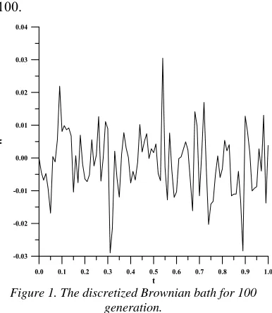
e W  s

Figure 1, presents the signal simulation of the discretized Brownian motion of the interval [0, 1]

with number of discritizations k 100, so that h 1/100.

0.0 0.1 0.2 0.3 0.4 0.5 0.6 0.7 0.8 0.9 1.0

t

-0.03 -0.02 -0.01 0.00 0.01 0.02 0.03 0.04

[image:7.612.323.516.107.329.2]

W

Figure 1. The discretized Brownian bath for 100 generation.

Therefore, using the approximate numerical solution using the VIM given by eq.(10), one may get:

xm+1(t;) xm(t;) 



₀t



x_m ( ; )s  x_m( ; )s 



sin(W_s( )) d s, t [0,1]

which may be simplified in connection with the trapezoidal rule to give for all m 0, 1, …:

xm+1(t;) xm(t;) 



₀tx_m ( ; ) ds  s 

0 ( ; ) d

t m

x s  s



+



₀tsin(W_s( )) d s

xm(0;) 



₀tx_m( ; ) ds  s +



sin 0( ) 2sin 1( )

2 t t

h

W   W  



1

... 2sin ( ) sin ( )

k k

t t

W _ W

   

where h is the step size which is taken in this example with k (say k 100)and hence h 

T

k , ti (0,1]. The simulation process with Winner

process will yields the results presented in Table 1, which are given for t  0, 0.1, …, 1. In addition, Figure 2 provides graphical illustration for the exact and the first five approximate solutions.

(8)

3581

t Exact Solution x

Approximate solution x1

0.0 1 1 1 1 1 1

0.1 0.90474 0.89988 0.90478 0.90451 0.90441 0.90431

0.2 0.81885 0.80011 0.82021 0.81897 0.81913 0.81922

0.3 0.74103 0.70021 0.74536 0.74101 0.74151 0.74164

0.4 0.67001 0.59967 0.67947 0.66858 0.66942 0.66912

0.5 0.60638 0.49979 0.62468 0.60372 0.60619 0.60581

0.6 0.54861 0.39974 0.57963 0.54348 0.54873 0.54794

0.7 0.4964 0.29973 0.54465 0.48734 0.49722 0.49569

0.8 0.44868 0.19923 0.51908 0.43334 0.45008 0.447

0.9 0.40537 0.0986 0.50346 0.38126 0.40806 0.40256

1.0 0.36667 1.20215103 _0.49848 _0.33241 _0.37312 _0.36432

0.0 0.1 0.2 0.3 0.4 0.5 0.6 0.7 0.8 0.9 1.0

t

0.0 0.1 0.2 0.3 0.4 0.5 0.6 0.7 0.8 0.9 1.0

Solut

ion

Exact solution x

Approximate solution x1

Approximate solution x3 Approximate solution x4

[image:8.612.92.304.83.470.2]

Figure 2. Comparison between the exact and the first five approximate solutions of example 1.

Example 2:

To solve the RODE:

2

d

sinh( ( ))

d t

x

x W

t     , x(t0,)  1, t [0,1] Therefore, using the approximate numerical solution using the VIM given by eq.(10), one may get:

xm+1(t;) xm(t;) 



₀t



x_m ( ; )s  



2_{( ; ) sinh(} _{( )) d}

m s

x s   W  s, t [0,1]

which may be simplified in connection with the trapezoidal rule to give:

xm+1(t;) xm(t;) 



₀tx_m ( ; ) ds  s 

2 0 ( ; ) d t

m

x s  s



+



₀tsinh(W_s( )) d s

xm(0;) 



₀tx_m2( ; ) ds  s +



sinh 0( ) 2sinh 1( )

2 t t

h

W   W  



1

... 2sinh ( ) sinh ( )

k k

t t

W _ W

    ,

m 0, 1, …

where h is the step size which is taken in this

example with k 100 and hence h T

(9)

[image:9.612.88.521.111.277.2]

3582

Table 2. The first six approximate solutions of example 2 using the modified VIM.

t Approximate solution x1

0.0 1 1 1 1 1 1

0.1 0.89988 0.90969 0.90895 0.90888 0.90879 0.90869

0.2 0.80011 0.83752 0.83324 0.83371 0.83376 0.83384

0.3 0.70021 0.78131 0.76811 0.76996 0.7699 0.77004

0.4 0.59967 0.73822 0.70946 0.71406 0.71326 0.71316

0.5 0.49979 0.70807 0.65751 0.66764 0.66593 0.66605

0.6 0.39974 0.68769 0.60882 0.62746 0.62392 0.62434

0.7 0.29973 0.67538 0.56245 0.59316 0.58671 0.58773

0.8 0.19923 0.66853 0.5167 0.56318 0.55232 0.55415

0.9 0.0986 0.66559 0.47152 0.53775 0.52092 0.52403

[image:9.612.98.382.310.681.2]

1.0 0.00152 0.66514 0.42713 0.51736 0.49291 0.4981

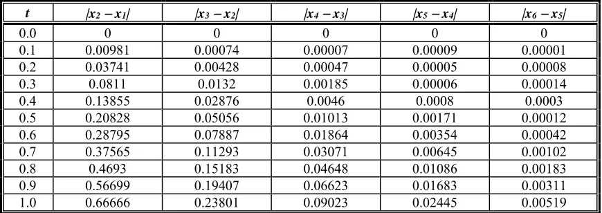
Table 3. The absolute error between the successive approximate solutions of example 2.

t |x2 x1| |x3 x2| |x4 x3| |x5 x4| |x6 x5|

0.0 0 0 0 0 0

0.1 0.00981 0.00074 0.00007 0.00009 0.00001

0.2 0.03741 0.00428 0.00047 0.00005 0.00008

0.3 0.0811 0.0132 0.00185 0.00006 0.00014

0.4 0.13855 0.02876 0.0046 0.0008 0.0003

0.5 0.20828 0.05056 0.01013 0.00171 0.00012

0.6 0.28795 0.07887 0.01864 0.00354 0.00042

0.7 0.37565 0.11293 0.03071 0.00645 0.00102

0.8 0.4693 0.15183 0.04648 0.01086 0.00183

0.9 0.56699 0.19407 0.06623 0.01683 0.00311

1.0 0.66666 0.23801 0.09023 0.02445 0.00519

0.0 0.1 0.2 0.3 0.4 0.5 0.6 0.7 0.8 0.9 1.0

t

-0.1 0.0 0.1 0.2 0.3 0.4 0.5 0.6 0.7 0.8 0.9 1.0

So

lu

ti

on

Figure 3. Comparison between first six approximate solutions of example 2.

7. CONCLUSIONS AND FUTURE WORK

The proposed approach followed in this paper is very efficient for solving stochastic and RODEs, which give reliable results for such type of problems consisting of Wiener process in comparison with the exact solution of example 1 (test example) or the absolute error between the successive approximate solutions of example 2. This approach may be used effectively to solve other type of problems which are given in operator form, which are so difficult to handle and then integrated.

[image:9.612.89.524.311.465.2]

(10)

3583

REFERENCES

[1] L Arnold, Stochastic Differential Equations; Theory and Application, John-Wiley and Sons, Inc., 1974.

[2] L. Arnold, Random Dynamical Systems, Springer,Berlin, 1998.

[3] Y. Asai, Numerical Methods for Random Ordinary Differential Equations and their Applications in Biology and Medicine. Dissertation, Institute für Mathematik, Goethe Universität, Frankfurt am Main, 2016.

[4] X. Han and P. Kloeden, Random Ordinary Differential Equations and Their Numerical Solution, Springer, Nature, Singapore, 2017. [5] L. C. Evans, An Introduction to Stochastic

Differential Equation, Version 12, Lecture Notes, Short Course at SIAM Meeting, July, 2006.

[6] A. Fridman, Stochastic Differential Equations and Applications, Vol.1, Academic Press, Inc., 1975.

[7] J. Jeisman, Estimation of the Parameters of Stochastic Differential Equations, Ph.D. Thesis, Business Queensland University of Technology, Australia, 2005.

[8] A. Röble, Runge-Kutta Methods for Numerical Solution of Stochastic Differential Equations, Ph.D. Thesis, Department of Math, technology University, Germany, 2003.

[9] D. Strizake, Stochastic Processes and Models. Oxford University Press, Inc., New-York, 2003.

[10]J. C. Cortés, L. Jódar, L. Villafuerte, Numerical Solution of Random Differential Equations: A Mean Square Approach, Math. and Compute Modeling, 45 (2007), pp.757-765.

[11]J. C. Cortés, L. Jódar, L. Villafuerte and R. Company, Numerical Solution of Random Differential Models, Math. and Computer Modeling, 54 (2011),pp. 1846-1851.

[12]A. R. Khudair, A. A. Ameen and S. L. Khalaf, Mean Square Solution of Second-Order Random Differential Equations by Using Variational Iteration Method, Applied Math. Sciences, Vol.5, 2011, No.51, pp. 2505-2516. [13]A. R. Khudair, A. A. Ameen and S. L. Khalaf,

Mean Square Solution of Second-Order Random Differential Equations by Using

Adomian Decomposition Method, Applied Math. Sciences, Vol.5, No.51, 2011, pp. 2521-2535.

[14]R. Farnoosh, H. Rezazadeh, A. Sabhani and D. Ebrahimibagha, Numerical Solution of Second Order Stochastic Differential Equation with Gaussian Random Parameters, Journal of Linear and Topological Algebra, Vol.2, 2013, pp. 229-241.

[15]K. Nauri and H. Ranjhar, Mean Square Convergence of the Numerical Solution of Random Differential Equations, Journal of Math., Vol.12, Issue 3, 2015, pp. 1123-1140 [16]A. R. Khudair, S. A. Haddad and S. L. Khalaf,

Improve the Mean Square Method of Second-Order Random Differential Equations by Using Homotopy Analysis Method, British Journal of Math. and Computer Science, 16 (5), 2016, pp.1-14.

[17]F. Tchier, C. Vetre and F. Vetro, Solution to Random Differential Equations with Boundary Conditions, Electronic Journal of Differential Equation, Vol.2017, 2017, pp. 1-12.

[18]P. E. Kloeden and E. Platen, “Numerical Solutions of Stochastic Differential Equations”, Springer, Berlin. 1992.

[19]K. H. Al-Jizani, N. A. Ahmad and F. S. Fadhel, Variational Iteration Method for Solving Riccati Matrix Differential Equations, Indonesian Journal of Electrical Engineering and Computer Science, 5(3), 2017, pp. 673-683.

[20]N. N. Hasan and F. S. Fadhel, Variational Iteration Method for Solving System of Fractional Order Ordinary Differential Equations, IOSR Journal of Meth., 10(6), 2014, pp.48-54.

[21]J. H. He, Variational Iteration Method; A Kind of Non-Linear Analytical Technique; Some Examples, International Journal of Non-Linear Mechanics, 34, 1999, pp.699-708.

[22]J. H. He, Variational Iteration Method for Autonomous Ordinary Differential System, Applied Math. Comput., 114 (23), 2000, pp.115-123.

(11)

3584 [24]J. H. He, Variational Iteration Method; Some

Recent Results and New Interpretations, Journal of Computational and Applied Mathematics, 207, 2007, pp. 3-17.

[25]K. H. Mohammedali, N. A. Ahmed and F. S. Fadhel, He’s Variational Iteration Method for Solving Riccati Matrix Delay Differential Equations of Variable Coefficients, AIP Conference Proceedings, 1830 (1), 2017. [26]A. M. Wazwas, A comparison between The

Variational Iteration Method and A Domain Decomposition Method, Journal of Computational and Applied Mathematics, 207, 2007, pp.129-136.