Quantifying uncertainty in urban flooding analysis considering hydro climatic projection and urban development effects

Hydrol. Earth Syst. Sci., 15, 617–633, 2011 www.hydrol-earth-syst-sci.net/15/617/2011/ doi:10.5194/hess-15-617-2011

© Author(s) 2011. CC Attribution 3.0 License.

Hydrology and

Earth System

Sciences

Quantifying uncertainty in urban flooding analysis considering

hydro-climatic projection and urban development effects

I.-W. Jung1,2, H. Chang1, and H. Moradkhani2

1_{Department of Geography, Portland State University, 1721 SW Broadway, Portland, OR 97201, USA} 2_{Department of Civil and Environmental Engineering, Portland State University, Portland, OR 97201, USA}

Received: 17 July 2010 – Published in Hydrol. Earth Syst. Sci. Discuss.: 5 August 2010 Revised: 6 February 2011 – Accepted: 7 February 2011 – Published: 22 February 2011

Abstract. How will the combined impacts of land use change, climate change, and hydrologic modeling influence changes in urban flood frequency and what is the main un-certainty source of the results? Will such changes differ by catchment with different degrees of current and future ur-ban development? We attempt to answer these questions in two catchments with different degrees of urbanization, the Fanno catchment with 84% urban land use and the Johnson catchment with 36% urban land use, both located in the Pa-cific Northwest of the US. Five uncertainty sources – gen-eral circulation model (GCM) structures, future greenhouse gas (GHG) emission scenarios, land use change scenarios, natural variability, and hydrologic model parameters – are considered to compare the relative source of uncertainty in flood frequency projections. Two land use change scenarios, conservation and development, representing possible future land use changes are used for analysis. Results show the highest increase in flood frequency under the combination of medium high GHG emission (A1B) and development sce-narios, and the lowest increase under the combination of low GHG emission (B1) and conservation scenarios. Although the combined impact is more significant to flood frequency change than individual scenarios, it does not linearly increase flood frequency. Changes in flood frequency are more sensi-tive to climate change than land use change in the two catch-ments for 2050s (2040–2069). Shorter term flood frequency change, 2 and 5 year floods, is highly affected by GCM structure, while longer term flood frequency change above 25 year floods is dominated by natural variability. Projected flood frequency changes more significantly in Johnson creek than Fanno creek. This result indicates that, under expected

Correspondence to: H. Chang ([email protected])

climate change conditions, adaptive urban planning based on the conservation scenario could be more effective in less de-veloped Johnson catchment than in the already dede-veloped Fanno catchment.

1 Introduction

large uncertainty, identifying potential changes in flood risk according to climate and land use changes is an important area of concern to water resource managers and land use planners (Hine and Hall, 2010).

For mitigation of and protection from potential flood risk in urban areas, we need to improve our understanding of the possible impacts of the ubiquitous uncertainty of urban flood projection. This uncertainty stems from several sources; in-ternal variability of the climate system, future GHG and aerosol emissions, the translation of these emissions into climate change by GCMs, spatial and temporal downscal-ing, and hydrological modeling (Bates et al., 2008). Un-certainty will not be radically removed or reduced until the development of the new technology of climate and hydro-logic modeling based on additional observation of hydrom-eteorological variables, such as soil moisture, snow, actual evapotranspiration, and groundwater. This uncertainty com-plicates the accurate interpretation of climate impact assess-ment. Therefore, many researchers have attempted to quan-tify the irreducible uncertainty in hydrologic streamflow pro-jections (New et al., 2007; Wilby, 2005; Chang and Jung, 2010; Kingston and Taylor, 2010), low flow (Wilby and Har-ris, 2006), flooding (Booij, 2005; Kay et al., 2009; Raff et al., 2009; Moradkhani et al., 2010), and drought (Ghosh and Mujumdar, 2007; Mishra and Singh, 2009). Despite substan-tial effort of previous studies, however, large uncertainty in climate impact studies still remain (Bates et al., 2008).

Floods in urban areas are controlled by the integrated con-dition of geophysical characteristics, urban infrastructure, drainage system, and hydro-climatologic regime (Epting et al., 2009). Thus, different levels of urban development could lead to different hydrologic responses among catchments, though they are under identical climate change (Franczyk and Chang, 2009). Kay et al. (2009) investigated the uncer-tainty in climate change impact on flood frequency for two catchments in England, showing that uncertainty can vary significantly between catchments that have different rain-fall regimes and topographic characteristics. Prudhomme and Davies (2009) reported similar findings for four catch-ments in Britain. Additionally, the combined effects of cli-mate change and anthropogenic land use change significantly aggravate the accuracy of hydrologic prediction associated with overall urban environmental management (Brath et al., 2006; Choi, 2008; Franczyk and Chang, 2009; Praskievicz and Chang 2009a; Tu, 2009). However, relatively few studies have examined the combined effects of climate change and urban development on the uncertainty of urban flood projec-tions in catchments with different degrees of urban develop-ment. This study attempts to fill this gap using two future land use change scenarios projected under two GHG emis-sion scenarios.

The three research questions are: (1) What are the main sources of uncertainties affecting the changes in urban flood frequency? (2) How will the combined impacts of land use change and climate change influence changes in flood

33 1

2

Fig. 1. Fanno and Johnson Creek catchment boundary, river network, and the Portland 3

urban growth boundary (UGB) 4

5

Fig. 1. Fanno and Johnson Creek catchment boundary, river net-work, and the Portland urban growth boundary (UGB).

frequency? and (3) How is flood frequency projected to change in two urban catchments with different degrees of ur-ban development for the 2050s (2040–2069) with respect to the reference period 1960–1989? This paper can contribute to a better understanding of the combined impact of climate and land use changes on urban flood frequency, and is ex-pected to help decision makers with practical urban planning and management to mitigate potential flood damage in urban areas in a changing climate.

2 Methodology

2.1 A process of flood frequency uncertainty analysis

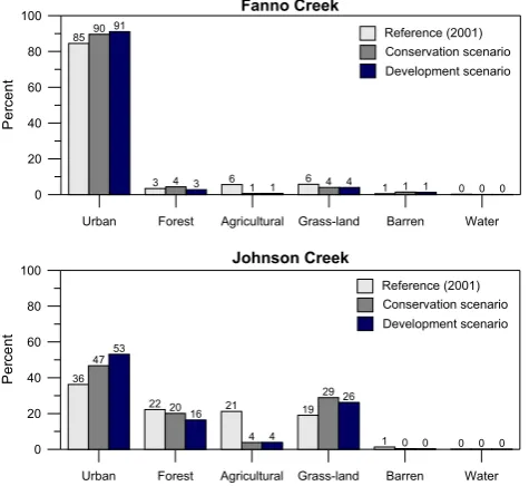
We investigate changes in flood frequency and the uncertain-ties associated with the combined effects of climate change and land use change in two catchments – Fanno Creek (80.5 km2) and Upper Johnson (hereafter Johnson) Creek (68.3 km2) in the Portland metropolitan area of Oregon, USA. The Fanno catchment is highly developed with 84% urban land use, and the Johnson catchment is moderately de-veloped with 36% urban land use in 2001 (see Fig. 1).

To quantify uncertainty in flood frequency change, this study considers five uncertainty sources; GCM structures, future GHG emission scenarios, future land use scenarios, hydrologic model parameters, and natural variability of the climate system. The GCM simulations are downscaled using the delta method to correct the bias between simulated and observed precipitation and temperature, which is attributed to scale mismatch between GCMs and catchment hydrologic models, as well as the lack of sub-grid scale climate dynam-ics such as orographically convective precipitation (Im et al., 2010).

I.-W. Jung et al.: Quantifying uncertainty in urban flooding analysis considering hydro-climatic projection 619 Precipitation Runoff Modeling System (PRMS), a

physically-based, deterministic, and semi-distributed model, is employed to simulate daily runoff changes and resulting changes in flood frequency under different climate and land use conditions. PRMS has been applied successfully in sev-eral regions with varying climate and land use (Bae et al., 2008a; Clark et al., 2008; Hay et al., 2006; Qi et al., 2009; Viney et al., 2009). To better understand the wide array of individual and combined factors that can affect the hydro-logic response in a watershed system, Risley et al. (2010) employed PRMS, driven by GCM outputs, in 14 watersheds across the US, and conducted a comparative statistical anal-ysis on the outputs. In the Willamette River basin, Ore-gon, PRMS has been applied in a water quality study (Lae-nen and Risley, 1997) and in a climate change impact study (Chang and Jung, 2010). To consider PRMS model parame-ter uncertainty, we extract acceptable parameparame-ter sets based on the Nash-Sutcliffe efficiency (NSE) criterion that esti-mates the degree of closeness between observed and simu-lated streamflow. Latin Hypercube Sampling is employed to efficiently sample the PRMS parameter sets within plausible ranges. A similar approach was undertaken by Wilby and Harris (2006).

It is also important to find whether the changes in flood frequency for the future period are larger than the natural (or model internal) climate variability (Hagemann and Ja-cob, 2007). It is especially likely that precipitation change derived from different initial conditions of GCMs could lead to different interpretation of the results due to large natural internal variability. To estimate natural climate variability, we employ the moving block Bootstrap resampling method (Ebtehaj et al., 2010), which produces a large number of new climate series through random selection of observed climate data. This method allows us to explore the range of different flood frequencies that could be obtained by our finite sam-pling of the internal climate variability (Kay et al., 2009). The US Geological Survey’s PeakFQ program (Flynn et al., 2006) is applied to estimate flood frequency with different recurrence intervals such as 2, 5, 10, 25, 50, and 100 years. To represent realistic future land use changes, we use two land use change scenarios: the conservation and the devel-opment scenarios, developed by the PNWERC (2002), these are both compared with 2001 land use. Further details of the data and methods used in this study are given in the following sections.

2.2 Study area and data

Fanno creek and the Johnson creek are important resources in the Portland metropolitan area, located in the valley of the Willamette River basin in Oregon (see Fig. 1). As a source of recreation and wildlife (Laenen and Risley, 1997), they contribute to the regional socio-economic and environmental systems. Two catchments are located in a modified marine temperate climate region in which summers are warm and

34 1

2

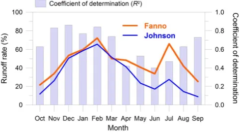
Fig. 2. Monthly runoff rate (%) that indicates the ratio of monthly runoff to monthly 3

precipitation for 2000-2006 and monthly coefficient of determination between the 4

Fanno daily streamflow (USGS 14206950) and the Johnson daily streamflow (USGS 5

14211500) 6

7

Fig. 2. Monthly runoff rate (%) that indicates the ratio of monthly runoff to monthly precipitation for 2000–2006 and monthly coefficient of determination between the Fanno daily streamflow (USGS 14206950) and the Johnson daily streamflow (USGS 14211500).

dry but winters are cold and wet. More than 80% of the an-nual precipitation occurs from October through May and less than 10% precipitation falls during July and August (Prask-ievicz and Chang, 2009b). This seasonality of precipitation causes periodic flooding and companying travel disruptions in winter (Chang et al., 2010).

In our study areas, most precipitation is in the form of rainfall. Unusual snow melts quickly during subsequent rain storms (Lee and Snyder, 2009). Therefore, the surface hy-drology of these regions is highly dominated by frequent rainfall. Although Fanno and Johnson are close to each other and have identical climate conditions, they show dif-ferent hydrologic regimes. Fanno shows a higher runoff ra-tio, defined as the ratio of total monthly runoff to precipi-tation, than Johnson for most months except March, which shows almost the same runoff ratio value in both catchments (see Fig. 2). Monthly runoff rates show the highest inter-basin differences in the dry season (June–August). This is attributed to different infiltration mechanisms as well as to geographic characteristics such as slope, soil, and shape of the catchment. Due to different geology and soils, precipita-tion in Fanno is less infiltrated and rapidly reaches the river, while the more infiltrated precipitation in Johnson is evapo-rated in warm and dry climate conditions. In the wet season (November–March), continuing rainfall results in saturated soil condition that can behave like an impervious surface, so differences in the monthly runoff rate are smaller than those of the dry season. The coefficient of determination of daily streamflow between the two catchments also shows higher linear relations (above 0.74) for the wet season and lower re-lations (below 0.63) for the dry season (see Fig. 2).

(NOAA COOP, 2010) for 1958–2006, and streamflow data are collected from the USGS National Water Information System (USGS NWIS, 2010) for 2000–2006. To delineate hydrologic response units (HRU) and estimate PRMS pa-rameters related to geographic layers, 10 m Digital Elevation Model (DEM) (ODGMI, 2010), soil map (NRCS, 1986), and land cover (PNWERC, 2002) are used.

2.3 Climate simulations and downscaling methods

Generally, the coupled atmosphere-ocean general circulation models (GCMs) are the best tools for projecting future cli-mate in response to GHG emission forcing. GCMs have di-verse horizontal and vertical grid resolutions, climate process description and approximation, parameterization of subgrid-scale phenomena, and initial condition (Randall et al., 2007). These different structures among GCMs cause the wide vari-ations and biases in regional climate reproduction and pro-jection (e.g., Im et al., 2011). Some GCMs fail to simulate regional inter-annual or decadal climate variability, which are important drivers of specific regional climate.

To estimate GCM performance in the Pacific Northwest, Mote and Salath´e (2010) rank the 20 GCMs, implemented in IPCC AR4, based on 20th century bias, a global performance index (Achuta Rao and Sperber, 2006), and North Pacific variability of temperature, precipitation, and sea-level pres-sures (Mote and Salath´e, 2010). The North Pacific variability represents the teleconnection effects of El Ni˜no Southern Os-cillation (ENSO) and Pacific Decadal OsOs-cillation (PDO) and other large-scale climate processes over the Pacific North-west (Hamlet et al., 2010). Based on the study of Mote and Salath´e (2010), this study selects the three best GCMs, which are CNRM-CM3, ECHAM5/MPI-OM, and ECHO-G. Better GCM performance at simulating historical climate does not inevitably indicate a realistic projection under GHG forcing. However, if a GCM has poor performance for current im-portant climate variability in the region, the derived regional changes for future should also be misleading (Prudhomme et al., 2002). No downscaling method can completely cor-rect for the GCM’s errors. Additionally, this approach pro-vides some useful information such as weighted factor of GCM simulations (e.g., Tebaldi et al., 2005), and reducing ensemble numbers for future climate projection (e.g., Mote and Salath´e, 2010).

This study uses two GHG emission scenarios, the A1B and B1 emission scenarios. Most global climate modeling groups generally employ A2, the A1B and B1 GHG emis-sion scenarios (Randall et al., 2007) as high, medium and low emission scenarios for the 21st century, respectively. We fo-cus on mid-century change for 2040–2069, in which period A2 and A1B show similar GHG emission forcing. There-fore, A1B and B1 emission scenarios can cover high and low GHG emission conditions. The climate simulation of three GCMs with two GHG emission scenarios are obtained from the World Climate Research Programme’s (WCRP’s)

Coupled Model Intercomparison Project phase 3 (CMIP3) multi-model dataset (WCRP CMIP3, 2010).

To downscale three GCM simulations with two emission scenarios, we use a simple delta method, which has widely been used in climate change impact studies (e.g., Lettenmaier et al., 1999; Wilby and Harris, 2006; Loukas et al., 2007; Graham et al., 2007; Kay et al., 2009; Choi et al., 2009). This method first calculates monthly precipitation and tem-perature differences between the reference and future GCM simulations. Then, the obtained monthly differences between the two periods are applied to historical daily data for the reference period by adding monthly absolute differences for temperature and by multiplying percent differences for pre-cipitation. This method can preserve the spatial and temporal variation of observation and remove the bias of GCM simula-tions. However, the delta method does not capture changes in precipitation and temperature variability from climate mod-els and does not allow for more complex changes in daily ex-treme of precipitation and temperature (Hamlet et al., 2010). Therefore, changes in day-to-day variability of climate sim-ulations are not taken into account in this study. This could lead to an underestimation of future flood frequency change. 2.4 Hydrologic model and parameter uncertainty

The PRMS model, Modular Modeling System (MMS) ver-sion developed by US Geological Survey (Leavesley and Stannard, 1996), is used in this study. This model simu-lates a water balance for each day and an energy balance for each half-day in each Hydrologic Response Unit (HRU), which is assumed to be homogeneous in its hydrologic re-sponse to given climate and land use conditions (Hay et al., 2009). A detailed description of the PRMS model structure is found in Leavesley et al. (2005). PRMS has seven parameters which are directly associated with land use change (see Table 1). Seasonal vegetation cover density (covden sum, covden win) and cover type (cov type) affect the amount of interception on HRUs. The seasonal vege-tation cover density is determined by different leaf loss of cover types, such as grass, shrub, deciduous and coniferous trees (Viger and Leavesley, 2007, p. 99). Maximum values of interception storage for each cover type are considered by season and precipitation type (wrain intcp, srain intcp, and snow intcp). Ratio of impervious surface area on HRU (hru percent imperv) is a more important parameter in land use change impact on flood analysis, because it is highly sen-sitive to urbanization. High impervious surface area in this model induces less infiltration to soil and more overland flow to streams, potentially increasing peak flow volume.

PRMS is a physically-based hydrologic model, so some parameters can be obtained from physiographic characteris-tics and land surface features of the watershed using GIS lay-ers, such as DEM, Land use, and Soil data (Chang and Jung, 2010). This study uses fixed parameters from GIS layers over time, except parameters related to land use. Snow effects are

I.-W. Jung et al.: Quantifying uncertainty in urban flooding analysis considering hydro-climatic projection 621

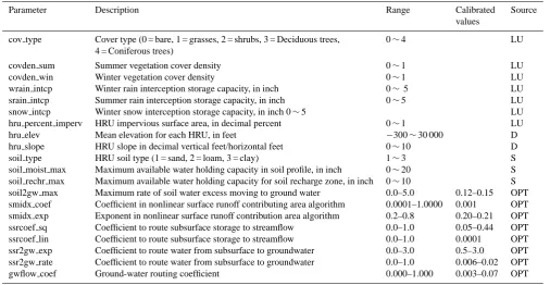
Table 1. PRMS model parameters for calibration. D: Digital elevation map, LU: Land use map, S: Soil map, OPT: Optimized (modified from Chang et al., 2010).

Parameter Description Range Calibrated Source

values

cov type Cover type (0 = bare, 1 = grasses, 2 = shrubs, 3 = Deciduous trees, 0∼4 LU

4 = Coniferous trees)

covden sum Summer vegetation cover density 0∼1 LU

covden win Winter vegetation cover density 0∼1 LU

wrain intcp Winter rain interception storage capacity, in inch 0∼5 LU

srain intcp Summer rain interception storage capacity, in inch 0∼5 LU

snow intcp Winter snow interception storage capacity, in inch 0∼5 LU

hru percent imperv HRU impervious surface area, in decimal percent 0∼1 LU

hru elev Mean elevation for each HRU, in feet −300∼30 000 D

hru slope HRU slope in decimal vertical feet/horizontal feet 0∼10 D

soil type HRU soil type (1 = sand, 2 = loam, 3 = clay) 1∼3 S

soil moist max Maximum available water holding capacity in soil profile, in inch 0∼20 S soil rechr max Maximum available water holding capacity for soil recharge zone, in inch 0∼10 S soil2gw max Maximum rate of soil water excess moving to ground water 0.0–5.0 0.12–0.15 OPT smidx coef Coefficient in nonlinear surface runoff contributing area algorithm 0.0001–1.0000 0.001 OPT smidx exp Exponent in nonlinear surface runoff contribution area algorithm 0.2–0.8 0.20–0.21 OPT

ssrcoef sq Coefficient to route subsurface storage to streamflow 0.0–1.0 0.05–0.44 OPT

ssrcoef lin Coefficient to route subsurface storage to streamflow 0.0–1.0 0.0001 OPT

ssr2gw exp Coefficient to route water from subsurface to groundwater 0.0–3.0 0.5–3.0 OPT

ssr2gw rate Coefficient to route water from subsurface to groundwater 0.0–1.0 0.006–0.02 OPT

gwflow coef Ground-water routing coefficient 0.000–1.000 0.003–0.07 OPT

minor in both catchments, so this study uses values recom-mended by Leavesley and Stannard (1996) for snow model-ing in PRMS. We calibrate eight parameters that are associ-ated with the timing and amount of runoff components (see Table 1). As in previous studies, streamflow simulation is most sensitive to these parameters (Bae et al., 2008b; Hay et al., 2009; Im et al., 2010; Chang and Jung, 2010).

LHS (McKay et al., 1979) is employed to sample the pa-rameters from plausible ranges. LHS is an efficient sampling method that provides larger sample space with less compu-tational effort comparable to those obtained from the con-ventional Monte Carlo simulation (Tang et al., 2007; Davey, 2008). LHS divides the feasible parameter space into equal intervals, so that at least one sample of each parameter set is selected randomly from each interval (Yang et al., 2010). To do an exhaustive search of behavioral parameters we de-cide to sample 20 000 parameters using LHS. These param-eter sets are used to dparam-etermine the closeness between daily simulated and observed streamflow for the period of 2000– 2006 in both catchments. The Nash-Sutcliffe (1970) non-dimensional model efficiency criterion (NSE) is used as a goodness of fit measure, with a value in excess of 0.6 indi-cating satisfactory fit between observed and simulated hydro-graphs (see Wilby, 2005; Choi and Beven, 2007). The NSE is generally more sensitive to high flow than low flow. Thus, an NSE score above 0.6 was considered appropriate for our flood frequency-focused study, since it mainly considers high

flows. This approach can show the relative importance of parameter uncertainty in climate impact studies, although it cannot cover total equifinality of parameters (Beven, 2001). Therefore, the whole range of parameter uncertainty on flood frequency estimation is probably larger than what is pre-sented in this study.

2.5 Natural variability

The natural variability of climate is the inherent internal fluc-tuation caused by combined effect of low-frequency (longer than 10 years) and high-frequency (shorter than 10 years) variability of nature (Wigley and Raper, 1990). The flood frequency analysis could be sensitive to the finite sampling within the natural climate variability (Kay et al., 2009). Therefore, it is essential that we analyze this sensitivity as an internal effect and anthropogenic climate change as external forcing. This will reveal the main source of uncertainty and indicate which source is a key controlling factor for future flood frequency change.

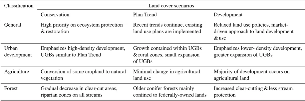
Table 2. Description of the three land cover scenarios used in this study to simulated land cover projections within the Fanno and Johnson Creek catchments by 2050 (Source: Hulse et al., 2004; Franczyk and Chang, 2009).

Classification Land cover scenarios

Conservation Plan Trend Development

General High priority on ecosystem protection Recent trends continue, existing Relaxed land use policies, market-& restoration land use plans are implemented driven approach to land development

& use

Urban Emphasizes high-density development, Growth contained within UGBs Emphasizes lower- density development, development UGBs similar to Plan Trend & rural zones, small expansion greater expansion of UGBs

of UGBs

Agriculture Conversion of some cropland to natural Minimal change in agricultural Majority of development occurs on

vegetation land use agricultural land

Forest Gradual decrease in clear-cut areas, Older conifer forests mainly Increased clear-cutting & less stream riparian zones on all streams confined to federally-owned lands protection

study used seasonally-based three month blocks, December– February (winter), March–May (spring), June–August (sum-mer), and September–November (fall), to demonstrate an-tecedent conditions and wet or dry season effect (Kay et al., 2009). For instance, the climate data of three months (December–February) in 1960 are randomly selected from any 3-month period between the water year 1960 and 1989. The selection of climate data with the same months is re-peated 30 times until the years of new series are the same of original time series. This process allows the selection of data for a specific water year which could be repeated or may not be used at all. Flood frequency using 100 resampled cli-mate series are compared to that obtained from original data. Also, the 100 resampled climate series are adjusted by the delta method described above to generate future climate con-ditions by the aforementioned three GCMs with two emis-sion scenarios.

2.6 Flood frequency analysis – PeakFQ

To estimate the impacts of climate and land use changes on flood frequency, this study used typical statistical flood frequency analysis of maximum annual flood series using the PeakFQ program. PeakFQ provides estimates of in-stantaneous maximum annual peak-flows having diverse re-currence intervals such as 2, 5, 10, 25, 50, 100, 200, and 500 years as annual-exceedance probabilities of 0.50, 0.20, 0.10, 0.04, 0.02, 0.01, 0.005, and 0.002, respectively. Here, a 100 year flood describes a flood that is believed to have a probability of being equal or exceeding 0.01 in any one year (Raff et al., 2009). This program was developed based on the Bulletin 17B guidelines of the Interagency Advisory Committee on Water Data (IACWD, 1982), which is recom-mended for use by Federal agencies in the US. Bulletin 17B assumes that flood frequency can be described by a log-Pearson Type 3 (LP3) probability distribution (Griffis and

Stedinger, 2007). Here, the LP3 distribution defines the prob-ability that any single annual peak flow will exceed a spec-ified streamflow. LP3 has three parameters: mean, standard deviation, and skew coefficient (Bobee and Ashkar, 1991). The skew coefficient is highly sensitive to the collected sam-ple data of annual maximum floods, so that PeakFQ pro-vides guidance on estimating the skew coefficient, such as the generalized skew from a digitized copy of the map in Bulletin 17B, the approach applied in this study.

2.7 Land use change scenarios

To consider possible future land use changes in both catch-ments, this study used two land-cover datasets developed by the Pacific Northwest Ecosystem Research Consortium (PN-WERC, 2002). The PNW-ERC provides three different land use scenarios for every 10 years of 2000–2050, namely, the conservation, the plan trend, and the development scenarios (see Table 2). These scenarios represent different future land-scapes, based on projected human population growth pat-terns and potential development characteristics throughout the Willamette River basin (Hulse et al., 2004). As shown in Table 2, the conservation scenario assumes that greater em-phasis on ecosystem protection and restoration will be im-plemented. The Plan Trend scenario assumes that current land use trends continue. The development scenario depicts greater expansion of urban growth boundaries (UGBs) with free rein to market forces across all components of the land-scape, resulting in sprawl urban development. More detailed description of these scenarios is found in Hulse et al. (2004). This study used the conservation and the development sce-narios as two extreme cases. A similar approach has been used in Franczyk and Chang (2009) and Praskievicz and Chang (2011).

I.-W. Jung et al.: Quantifying uncertainty in urban flooding analysis considering hydro-climatic projection 623 2.8 Comparison of uncertainty sources

To identify the main source of uncertainty, we compare the maximum range of flood frequency change according to each uncertainty source (Jung et al., 2010). For instance, to deter-mine the effect of GCM simulations (GCM structures), we first calculate the differences in flood frequency changes that are derived by different GCM simulations while holding the other data such as land use changes, emission scenarios, hy-drologic model parameters, and natural variability constant. We then rank these differences and determine the maximum value at the top 5%. The same methodology is repeated to determine the maximum range for each uncertainty source.

3 Results and discussion

3.1 Hydrologic model calibration

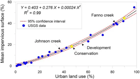
To calibrate PRMS model parameters, HRUs for the two catchments are delineated based on streamflow network, slope, aspect, and soil type. The geophysical parameters are extracted from DEM, land use, and soil GIS layers (see Table 1). The rest of the parameters (eight process param-eters) are calibrated using Rosenbrock’s (1960) automatic optimization method. The ratio of impervious surface area in HRU (hru percent imperv) is strongly related to land use change, as mentioned in Sect. 2.4. However, the land use layers of PNWERC do not provide the specific information of impervious surface area. They only describe some urban-related land use, such as residential, commercial, industrial, railroads, and roads. These land use categories contain both pervious and impervious surface areas. Therefore, if all ur-ban land uses are assumed to be impervious surface areas, flood frequency would be overestimated. To determine the ratio of impervious surface area to urban land use, we de-velop an empirical relation between urban land use (%) and mean impervious surface area (%) (see Fig. 3) based on the data set of Waite et al. (2008). Waite et al. (2008) used dif-ferent land use types, including mean impervious surface area, for 28 catchments in Oregon and Washington to es-timate the effect of urbanization on steam ecosystems. As shown in Fig. 3, the estimated regression equation shows a good fit between urban land use and mean impervious sur-face area (R2= 0.99). The regression coefficients are used to estimate percent impervious surface areas in each HRU (hru percent imperv) in PRMS modeling for these two urban catchments.

3.2 Projected future climate change and land use change

Changes in monthly precipitation show different patterns by GCMs and GHG emission scenarios, but the changes are similar in the two catchments (see Fig. 4). The CNRM-CM3 and the ECHAM5/MPI-OM simulations project slight

35 1

2

3 4

Fig. 3. Relation between urban land use (%) and mean impervious surface (%). Data are 5

obtained from USGS Report 2006-5101-D (Waite et al., 2008, Table 1) 6

7

Fig. 3. Relation between urban land use (%) and mean impervious surface (%). Data are obtained from USGS Report 2006-5101-D (Waite et al., 2008, Table 1).

increases in winter (December, January, and February) pre-cipitation, while predicting drier summers (June, July, Au-gust, and September) as indicated by previous studies (e.g., Mote et al., 2003; Graves and Chang, 2007; Chang and Jung, 2010). In the study catchments, winter precipitation is closely related to flood events. Therefore, rising water tables resulting from an increase of winter precipitation and soil moisture content are likely to lead to more frequent flooding in this region. However, the ECHO-G projects a slight de-crease in winter precipitation. These different precipitation projections contribute to uncertainty in flood frequency anal-ysis. Climate change projection for monthly temperatures ranges from +0.3◦C increase in February (CNRM-CM3, B1) to +6.1◦C in August (ECHO-G, A1B) for the 2050s (not shown).

36

Jan Feb Mar Apr May Jun Jul Aug Sep Oct Nov Dec -80 -40 0 40 80 Chang e i n pr ec ip itat io

n (%) CNRM-CM3 ECHO-G ECHAM5/MPI-OM

Fanno Creek - A1B scenario

Johnson Creek - A1B scenario

Jan Feb Mar Apr May Jun Jul Aug Sep Oct Nov Dec -80 -40 0 40 80 Chang e i n pr ec ip itat io

n (%) CNRM-CM3 ECHO-G ECHAM5/MPI-OM

Fanno Creek - B1 scenario

Johnson Creek - B1 scenario

Jan Feb Mar Apr May Jun Jul Aug Sep Oct Nov Dec -80 -40 0 40 80 C hange in p re cip ita tio

n (%) CNRM-CM3 ECHO-G ECHAM5/MPI-OM

Jan Feb Mar Apr May Jun Jul Aug Sep Oct Nov Dec -80 -40 0 40 80 Cha nge i n pre ci pi tat ion (%)

CNRM-CM3 ECHO-G ECHAM5/MPI-OM

1

2

Fig. 4. Changes in precipitation according to three GCMs and two emission scenarios in

3

Fanno Creek and Johnson Creek catchments.

4

5

6

Fig. 4. Changes in precipitation according to three GCMs and two emission scenarios in Fanno Creek and Johnson Creek catchments.

37

Urban Forest Agricultural Grass-land Barren Water 0 20 40 60 80 100 Pe rc e n t 85

3 6 6

1 0

90

4

1 4 1 0

91

3 ₁ 4 _{1 0}

Reference (2001) Conservation scenario Development scenario

Fanno Creek

Urban Forest Agricultural Grass-land Barren Water 0 20 40 60 80 100 Pe rce n t 36

22 21 ₁₉

1 0 47 20 4 29 0 0 53 16 4 26 0 0 Reference (2001) Conservation scenario Development scenario Johnson Creek 1 2

Fig. 5. Land use categories (%) for reference land use in 2001 and two future land use 3

change scenarios for the 2050s 4

5

Fig. 5. Land use categories (%) for reference land use in 2001 and two future land use change scenarios for the 2050s.

3.3 Projected flood frequency

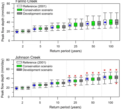
Figure 6 shows the range of flood frequency at the refer-ence and future climate change conditions, excluding land use change effects. The reference period only considers the natural variability impact. Hence, the two future peri-ods represent impacts of climate change on flood frequency

caused by the combined conditions of climate change and natural variability. The effect of climate change is much more dominant in both catchments as compared with nat-ural variability (taller box and whisker). The t-test results show that the flood frequency of all return periods signifi-cantly changes due to climate change at the 95% confidence level (see Table 3). The GHG emission scenarios are only significantly different for 2-year flood frequency. The cli-mate change impact on flood frequency between both ments is similar. This is attributed to the fact that the catch-ments are located in same climate region in the Willamette Valley and analyses are made using data derived from coarse scale GCM simulations. In a contrasting case study, Kay et al. (2009) show different responses between two distant catchments in UK using regional climate model (RCM) sim-ulations. They show that one catchment is highly dominated by natural variability, while the other catchment is strongly affected by climate change. Hulme et al. (1999) explain that if a region is more dominated by natural variability than by climate change, adaptation management that takes into ac-count natural variability may be sufficient to withstand cli-mate change. Our results show that future flood management in the Fanno and Johnson creek catchments should consider climate change impact as well as historical natural climate variability.

As shown in Fig. 7, the natural variability impact is much greater than future land use change impact. The variation in flood frequency caused by land use change is similar to that due to natural variability in both catchments. However, un-der the development scenario, short-term floods (2 and 5 year floods) in Johnson Creek show significant changes at the 95%

I.-W. Jung et al.: Quantifying uncertainty in urban flooding analysis considering hydro-climatic projection 625 38 0 20 40 60 80 Peak fl ow de pth (mm/d ay)

2 5 10 25 50 100

Return period (years) Fanno Creek Natural variability A1B scenario B1 scenario 0 20 40 60 80 Peak fl ow d epth (mm/day)

2 5 10 25 50 100

Return period (years) Johnson Creek Natural variability A1B scenario B1 scenario 1 2 3

Fig. 6. Variation of flood frequency by climate change scenarios, with recurrence 4

intervals of 2, 5, 10, 25, 50, and 100 years for the 2050s with respect to the reference 5

period of 1960-1989. The blue dot indicates flood frequency using observed climate 6

data and symbol (x) indicates outliers. 7

8

Fig. 6. Variation of flood frequency by climate change scenarios, with recurrence intervals of 2, 5, 10, 25, 50, and 100 years for the 2050s with respect to the reference period of 1960–1989. The blue dot indicates flood frequency using observed climate data and sym-bol (x) indicates outliers.

confidence level (see Table 3). This might indicate that no-table land use change in less developed catchment could lead to significantly more frequent bankfull flooding, although the natural variability effect is more pronounced for larger flood events. The median values of flood frequency under the de-velopment condition are slightly higher than those of the con-servation scenario. Also, shorter term floods increase more than longer term floods.

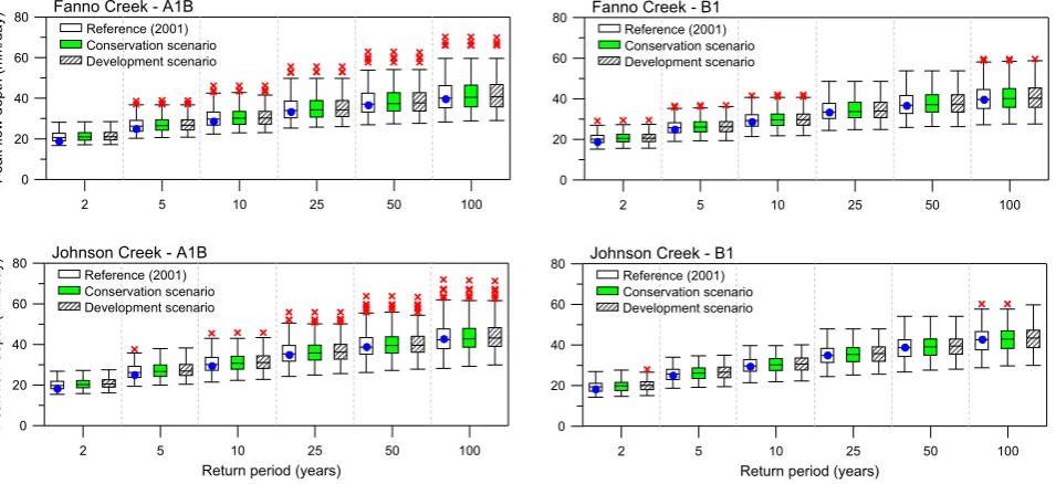
For the combined impact of climate and land use changes, flood frequency at the six different return periods increases slightly, though each change had high variations (Fig. 8). The range of flood frequency change gradually increases from shorter term floods to longer term floods. The variations under the A1B scenario are larger than those under the B1 scenario in both catchments. Since variation is high, an in-terpretation of the flood frequency impact of each scenario solely based on Fig. 8 is difficult. Accordingly, we calculated ensemble mean value of flood frequency change for each sce-nario.

Figure 9 shows the ensemble mean of relative changes of flood frequency under two GHG emission, two land cover change, and the combined scenarios (four) that are calcu-lated from the reference flood frequency. The A1B scenario shows the biggest change among the separate emission and land cover scenarios in both catchments. In the Fanno creek catchment, ensemble results of all 8 scenarios show higher changes than those caused by natural variability. However, in Johnson creek, the natural variability impact becomes more significant than the B1 and land cover change scenarios for

39 0 20 40 60 80 Peak fl ow de pth (mm/d ay)

2 5 10 25 50 100

Return period (years) Fanno Creek Reference (2001) Conservation scenario Development scenario 0 20 40 60 80 Peak fl ow d epth (mm/day)

2 5 10 25 50 100

Return period (years) Johnson Creek Reference (2001) Conservation scenario Development scenario 1 2

Fig. 7. Variation of flood frequency by land use change scenarios, with recurrence 3

intervals of 2, 5, 10, 25, 50, and 100 years for the 2050s with respect to the reference 4

period of 1960-1989. The blue dot indicates flood frequency using observed climate 5

data, and symbol (x) indicates outliers. 6

7

Fig. 7. Variation of flood frequency by land use change scenarios, with recurrence intervals of 2, 5, 10, 25, 50, and 100 years for the 2050s with respect to the reference period of 1960–1989. The blue dot indicates flood frequency using observed climate data, and sym-bol (x) indicates outliers.

short-term flood frequency of less than 25 year floods. In all cases, the combined impacts on flood frequency are higher than those of natural variability in both catchments. Of the combined land use and climate scenarios, the A1B with de-velopment scenario induces the highest increase in flood fre-quency, and the B1 with conservation scenario induces the lowest increase in flood frequency. The shorter term flood frequencies are more sensitive to the combined scenarios than longer term ones (see Table 4). Further, the difference between A1B with development scenario and B1 with con-servation scenario is greater in Johnson than in Fanno (see % difference between the two scenarios in Fig. 9). For the long term extremes, the Johnson creek shows significant dif-ference between the A1B with development scenario (6.6% difference) and the B1 with conservation scenario (3.4% dif-ference) (see Table 4).

40

0 20 40 60 80

P

eak flow

d

epth (mm/day)

2 5 10 25 50 100

Fanno Creek - A1B

Reference (2001) Conservation scenario Development scenario

0 20 40 60 80

Peak flow

depth (mm

/d

ay)

2 5 10 25 50 100

Return period (years)

Johnson Creek - A1B

Reference (2001) Conservation scenario Development scenario

0 20 40 60 80

2 5 10 25 50 100

Fanno Creek - B1

Reference (2001) Conservation scenario Development scenario

0 20 40 60 80

2 5 10 25 50 100

Return period (years)

Johnson Creek - B1

Reference (2001) Conservation scenario Development scenario

1

2

Fig. 8. Variation of flood frequency flows by combination of

land use change and

3

climate change scenarios

with recurrence intervals of 2, 5, 10, 25, 50, and 100 years for

4

the 2050s with respect to the reference period of 1960-1989. The blue dot indicates

5

flood frequency using observed climate data, and symbol (x) indicates outliers.

6

7

Fig. 8. Variation of flood frequency flows by combination of land use change and climate change scenarios with recurrence intervals of 2, 5, 10, 25, 50, and 100 years for the 2050s with respect to the reference period of 1960–1989. The blue dot indicates flood frequency using observed climate data, and symbol (x) indicates outliers.

41 1

2 5 10 25 50 100

0 4 8 12 16 20

Chang

e in

floo

d frequ

ency

(%) _A1B

B1 Conservation Development

A1B + Conservation A1B + Development B1 + Conservation B1 + Development

2 5 10 25 50 100

Return period (years) 0

4 8 12 16 20

Chang

e in flo

od freq

uency

(%)

Fanno Creek

Johnson Creek

A1B B1 Conservation Development

A1B + Conservation A1B + Development B1 + Conservation B1 + Development 4.1%

3.3%

3.0%

2.8% 2.7% 2.6%

6.6%

5.1%

4.5%

3.9% 3.6%

3.4% Natural variability

Natural variability

2 3

Fig. 9. Ensemble mean of changes (%) in flood frequency under different scenarios for 4

the 2050s with respect to the reference period of 1960-1989. 5

6

Fig. 9. Ensemble mean of changes (%) in flood frequency under different scenarios for the 2050s with respect to the reference period of 1960–1989.

I.-W. Jung et al.: Quantifying uncertainty in urban flooding analysis considering hydro-climatic projection 627

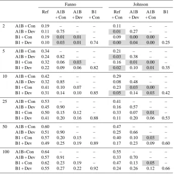
Table 3. t-test result of comparison between flood frequency change by GHG emission scenarios and land use change scenarios. Shaded value indicates significantp-value at the 95% confidence level.

Climate change Land use change

Fanno Johnson Fanno Johnson

Emission Ref A1B Ref A1B Land use Ref Con. Ref Con.

2 A1B 0.00 – 0.00 – Con. 0.25 – 0.06 –

B1 0.00 0.01 0.00 0.00 Dev. 0.15 0.77 0.00 0.22

5 A1B 0.00 – 0.00 – Con. 0.46 – 0.21 –

B1 0.00 0.06 0.00 0.01 Dev. 0.37 0.86 0.04 0.39

10 A1B 0.00 – 0.00 – Con. 0.57 – 0.33 –

B1 0.00 0.11 0.00 0.03 Dev. 0.46 0.86 0.11 0.54

25 A1B 0.00 – 0.00 – Con. 0.65 – 0.48 –

B1 0.00 0.16 0.00 0.07 Dev. 0.58 0.92 0.25 0.65

50 A1B 0.00 – 0.00 – Con. 0.69 – 0.58 –

B1 0.00 0.21 0.00 0.11 Dev. 0.64 0.94 0.35 0.70

100 A1B 0.00 – 0.00 – Con. 0.73 – 0.66 –

B1 0.00 0.24 0.00 0.15 Dev. 0.68 0.94 0.46 0.77

projections of urban flood risk, we need to develop possible climate change scenarios as well as land use change scenar-ios.

3.4 Comparison of five uncertainty sources

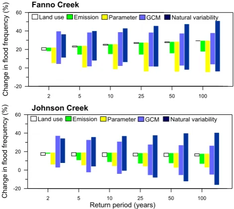
Figure 10 shows the relative variation (uncertainty) in flood frequency change projections under the combined impact of climate and land use change. Uncertainty due to land use change is the smallest in this study, except for the occurrence of 2 year floods at Johnson creek, although the Johnson’s range is larger than the Fanno’s. This could indicate that longer term floods could be less affected by land use change than climate change. However, this result also suggests that if land use at a catchment scale changes abruptly, the land use change will become a more significant uncertainty source than climate change for short term floods. Emission scenario uncertainty also shows a relatively smaller range than those of the other sources. The uncertainty from hydrologic pa-rameters is more significant at Fanno than Johnson, but it is smaller than uncertainty due to GCM and natural variability. GCM uncertainty strongly affects shorter term 2 and 5 year floods, while longer term 25, 50, and 100 year floods are more controlled by natural variability. This demonstrates that both uncertainty sources, GCMs and natural variability, are significant factors in urban flood frequency analysis. 3.5 Caveats of this study

This research deals with uncertainty in future flood frequency analysis in two distinct urban areas. We consider three un-certainty sources; climate projection (GCM structure, future

2 5 10 25 50 100

-20 0 20 40 60

Change in

fl

ood frequency (%

) _{Fanno Creek}

Johnson Creek

2 5 10 25 50 100

Return period (years) -20

0 20 40 60

Ch

an

ge

in

f

lood

f

requency (%)

Land use Emission Parameter GCM Natural variability

Land use Emission Parameter GCM Natural variability

1 2

Fig. 10. Comparison of variation in flood frequency change by each uncertainty source. 3

The vertical ranges show the 95% confidence interval. 4

Fig. 10. Comparison of variation in flood frequency change by each uncertainty source. The vertical ranges show the 95% confidence interval.

GHG emission scenario, and natural variability), urban de-velopment (different future land use planning scenarios), and hydrologic modeling (hydrologic model parameters). Our re-sults contribute to an understanding of the combined effects of hydro-climatic modeling and urban development effects on urban flood analysis. While we identify the relative mag-nitude of uncertainties arising from the sources mentioned above, there are remaining uncertainty sources, such as GCM

Table 4. t-test result of comparison between flood frequency change by combination of GHG emission scenarios and land use change scenarios. Shaded value indicates significant difference at the 95% confidence level.

Fanno Johnson

Ref A1B A1B B1 Ref A1B A1B B1

+ Con + Dev + Con + Con + Dev + Con

2 A1B + Con 0.19 – – – 0.11 – – –

A1B + Dev 0.11 0.75 – – 0.01 0.27 – –

B1 + Con 0.19 0.01 0.01 – 0.09 0.00 0.00 –

B1 + Dev 0.10 0.03 0.01 0.74 0.00 0.04 0.00 0.25

5 A1B + Con 0.34 – – – 0.21 – – –

A1B + Dev 0.24 0.82 – – 0.03 0.38 – –

B1 + Con 0.32 0.06 0.03 – 0.16 0.01 0.00 –

B1 + Dev 0.22 0.09 0.06 0.82 0.02 0.10 0.01 0.35

10 A1B + Con 0.42 – – – 0.29 – – –

A1B + Dev 0.32 0.85 – – 0.08 0.48 – –

B1 + Con 0.41 0.10 0.07 – 0.23 0.03 0.00 –

B1 + Dev 0.31 0.14 0.10 0.85 0.05 0.14 0.03 0.42

25 A1B + Con 0.53 – – – 0.41 – – –

A1B + Dev 0.45 0.90 – – 0.16 0.57 – –

B1 + Con 0.50 0.15 0.12 – 0.33 0.07 0.01 –

B1 + Dev 0.41 0.20 0.16 0.88 0.11 0.20 0.06 0.53

50 A1B + Con 0.60 – – – 0.47 – – –

A1B + Dev 0.51 0.90 – – 0.25 0.66 – –

B1 + Con 0.57 0.20 0.15 – 0.40 0.10 0.03 –

B1 + Dev 0.49 0.25 0.19 0.89 0.17 0.23 0.09 0.60

100 A1B+Con 0.64 – – – 0.55 – – –

A1B + Dev 0.57 0.91 – – 0.33 0.70 – –

B1 + Con 0.62 0.23 0.19 – 0.47 0.13 0.05 –

B1 + Dev 0.55 0.27 0.22 0.92 0.24 0.26 0.12 0.66

initial condition, downscaling method, and hydrologic model structure, which are not investigated in the current study. Therefore, our results should be cautiously interpreted along with other potential sources of uncertainties.

We carefully select the three best GCMs, but these GCMs do not necessarily project future climate accurately. Further-more, three GCMs are insufficient to cover the full range of GCM structure uncertainty. However, our results show the uncertainty caused by GCMs is higher than that due to other sources. This is consistent with the findings of previous stud-ies (e.g., Wilby and Harris, 2006; Kay et al., 2009). There-fore, the end-to-end effect of GCM uncertainty on flood fre-quency projection could be larger than that presented in this study, however, the relative magnitudes of the GCM struc-tural uncertainty might not vary. The uncertainties due to future GHG emissions are not fully considered as proposed in the IPCC storyline (IPCC, 2000).

Our results are also affected by the simple delta method for downscaling GCMs because this approach cannot consider changes in interannual or day-to-day variability of climate simulations (Im et al., 2010; Prudhomme and Davies, 2009).

Additionally, using a different NSE threshold value could have resulted in a wider or narrower parameter uncertainty range, although it would still not be significant compared to other uncertainty sources. However, more sophisticated methods and approaches in quantifying the parameter uncer-tainty relying on Sequential Monte Carlo (SMC) using en-semble filtering (Moradkhani et al., 2005a,b; Moradkhani and Sorooshian, 2008; Leisenring and Moradkhani, 2010; DeChant and Moradkhani, 2011; Montzka et al., 2011), Markov Chain Monte Carlo (MCMC) (e.g., Smith and Mar-shall, 2008; Vrugt et al., 2009) and Moving Block Boot-strap Sampling (MBBS) (Ebtehaj et al., 2010) can be em-ployed. Furthermore, we did not include uncertainties asso-ciated with climate data downscaling (Fowler et al., 2007; Im et al., 2010; Najafi et al., 2010a), and hydrologic model structure (Clark et al., 2008; Jiang et al., 2007; Bae et al., 2011; Najafi et al., 2010b). Recently, Najafi et al. (2010b) used Bayesian Model Averaging to quantify and minimize the uncertainty associated with hydrologic model structure and selection in the context of hydrologic climate change im-pact studies.

I.-W. Jung et al.: Quantifying uncertainty in urban flooding analysis considering hydro-climatic projection 629 Urban climate is controlled not only by global and regional

natural climate systems, but also by local urbanization ef-fects, such as the urban heat island, the urban canopy layer, and varying aerosol composition (Ntelekos et al., 2010). Ur-banization could significantly affect the precipitation clima-tology relating to flood events (Shepherd, 2005). Ntelekos et al. (2008) demonstrates that rainfall accumulations of 30% of the total extreme events are attributed to urbanization im-pacts in the Baltimore metropolitan area, Washington DC. Therefore, the interaction between global climate change and urban climatology is another important uncertainty source in urban climate impact studies.

In changing climate conditions, an assumption of station-arity in flood frequency analysis may not be valid (Milly et al., 2008; Smith et al., 2005). This study uses the PeakFQ based on the Bulletin 17B that assumes the constant distri-bution of flood events regardless of climate change. Some previous studies illustrate that a traditional approach to flood frequency estimation could not rely on stationarity assump-tions (Raff et al., 2009; Sivapalan and Samuel, 2009). Now, a robust methodology for incorporating projected climate in-formation into flood frequency analysis is needed.

4 Conclusions

This study examines the potential changes of flood frequency and the associated uncertainties in the two catchments ex-hibiting different levels of urbanization. Here, the important conclusions are summarized.

1. For the combined scenarios, GCM uncertainty highly affects shorter term extremes, while longer term ex-tremes are more controlled by natural variability. Hence, the uncertainties due to future GHG emission scenarios and land use change scenarios are less im-portant than natural variability. Also, hydrologic model parameter has less impact than natural variability and GCM structure in our uncertainty analysis.

2. The combined impacts of land use change and cli-mate change scenarios induce significant changes in the shorter term extremes in both catchments. Flood fre-quency change demonstrates the highest increase under the A1B with development scenario and the lowest in-crease under the B1 with conservation scenario. 3. In the 2050s period, flood frequency is projected to

slightly increase in both catchments, although there are substantial uncertainties. Changes in flood frequency are more sensitive to climate change (A1B scenario) than land use change. Land use change impact is only significant in the less developed Johnson catchment, which is projected to be more urbanized in the 2050s.

Acknowledgements. This research was supported by the Oregon

Transportation Research and Education Consortium (OTREC), the James F. and Marion L. Miller foundation and the Institute for Sustainable Solutions (formerly Center for Sustainable Processes and Practices) at Portland State University. We acknowledge the modeling groups, the Program for Climate Model Diagnosis and Intercomparison (PCMDI) and the WCRP’s Working Group on Coupled Modeling (WGCM) for their roles in making the WCRP CMIP3 multi-model dataset available. Support of this dataset is provided by the Office of Science, US Department of Energy. Two anonymous reviewers’ comments improved the clarity of our presentation. Thanks also go to Madeline Steele of Portland State University who carefully proofread the manuscript.

Edited by: J. Vrugt

References

Achuta Rao, K. and Sperber, K.: ENSO simulation in coupled ocean-atmosphere models: are the current models better?, Clim. Dynam., 27, 1–15, 2006.

Arnell, N. W.: Relative effects of multi-decadal climatic variability and changes in the mean and variability of climate due to global warming: future streamflows in Britain, J. Hydrol., 270(3–4), 195–213, 2003.

Bae, D. H., Jung, I. W., and Chang, H.: Long-term trend of pre-cipitation and runoff in Korean river basins, Hydrol. Process., 22(14), 2644–2656, 2008a.

Bae, D. H., Jung, I. W., and Chang, H.: Potential changes in Korean water resources estimated by high-resolution climate simulation, Clim. Res., 35(3), 213–226, 2008b.

Bae, D. H., Jung, I. W., and Lettenmaier, D. P.: Hydrologic uncertainties in climate change from IPCC AR4 GCM sim-ulations of the Chungju Basin, Korea, J. Hydrol., in press, doi:10.1016/j.jhydrol.2011.02.012, 2011.

Bates, B., Kundzewicz, Z. W., Wu, S., and Palutikof, J. P.: Cli-mate Change and Water. Technical Paper of the Intergovernmen-tal Panel on Climate Change (IPCC), Geneva, 1–210, 2008. Beven, K. J.: Calibration, validation and equifinality in hydrological

modeling, in: Model Validation: Perspectives in Hydrological Science, edited by: Anderson, M. G. and Bates, P. D., Wilby, Chichester, 43–44, 2001.

Bobee, B. and Ashkar, F.: The gamma family and derived distribu-tions applied in hydrology, Water Resources, Highlands Ranch, Colorado, 1991.

Booij, M. J.: Impact of climate change on river flooding assessed with different spatial model resolutions, J. Hydrol., 303(1–4), 176–198, 2005.

Brath, A., Montanari, A., and Moretti, G.: Assessing the effect on flood frequency of land use change via hydrological simulation (with uncertainty), J. Hydrol., 324(1–4), 141–153, 2006. Brun, S. E. and Band, L. E.: Simulating runoff behavior in an

urban-izing watershed, Computers, Environ. Urban Syst., 24(1), 5–22, 2000.

Chang, H. and Jung, I. W.: Spatial and temporal changes in runoff caused by climate change in a complex river basin in Oregon, J. Hydrol., 388(3–4), 186–207, 2010.

Chang, H., Franczyk, J., and Kim, C.: What is responsible for in-creasing flood risks? The case of Gangwon Province, Korea, Nat. Hazards, 48(3), 339–354, 2009.

Chang, H., Lafrenz, M., Jung, I. W., Figliozzi, M., Platman, D., and Pederson, C.: Potential impacts of climate change on flood-induced travel disruption: a case study of Portland in Oregon, USA, Ann. Assoc. Am. Geogr., 100(4), 938–952, 2010. Changnon, S. A. and Demissie, M.: Detection of changes in

stream-flow and floods resulting from climate fluctuations and land use-drainage changes, Climatic Change, 32(4), 411–421, 1996. Choi, H. T. and Beven, K.: Multi-period and multi-criteria model

conditioning to reduce prediction uncertainty in an application of TOPMODEL within the GLUE framework, J. Hydrol., 332, 316–336, 2007.

Choi, W.: Catchment-scale hydrological response to climate-land-use combined scenarios: A case study for the Kishwaukee River Basin, Illinois, Phys. Geogr., 29(1), 79–99, 2008.

Choi, W., Rasmussen, P. F., Moore, A. R., and Kim, S. J.: Simulat-ing streamflow response to climate scenarios in central Canada using a simple statistical downscaling method, Clim. Res., 40(1), 89–102, 2009.

Clark, M. P., Slater, A. G., Rupp, D. E., Woods, R. A., Vrugt, J. A., Gupta, H. V., Wagener, T., and Hay, L. E.: Framework for Understanding Structural Errors (FUSE): a modular framework to diagnose differences between hydrological models, Water Re-sour. Res., 44, W00B02, doi:10.1029/2007wr006735, 2008. Crooks, S. and Davies, H.: Assessment of land use change in the

Thames catchment and its effect on the flood regime of the river, Phys. Chem. Earth Pt. B, 26(7–8), 583–591, 2001.

Davey, K. R.: Latin Hypercube Sampling and pattern search in mag-netic field optimization problems, IEEE T. Magn., 44(6), 974– 977, 2008.

DeChant, C. and Moradkhani, H.: Radiance Data Assimilation for operational Snow and Streamflow Forecasting, Adv. Water Re-sour., 34, 351-364, 2011.

Ebtehaj, M., Moradkhani, H., and Gupta, H. V.: Improving robust-ness of hydrologic parameter estimation by the use of moving block bootstrap resampling, Water Resour. Res., 46, W07515, doi:10.1029/2009WR007981, 2010.

Epting, J., Romanov, D., Huggenberger, P., and Kaufmann, G.: In-tegrating field and numerical modeling methods for applied ur-ban karst hydrogeology, Hydrol. Earth Syst. Sci., 13, 1163–1184, doi:10.5194/hess-13-1163-2009, 2009.

Flynn, K. M., Kirby, W. H., and Hummel, P. R.: User’s Manual for Program PeakFQ Annual Flood-Frequency Analysis Using Bulletin 17B Guidelines: US Geological Survey, Techniques and Methods Book 4, Chapter B4, p.42, 2006.

Fowler, H. J., Blenkinsop, S., and Tebaldi, C.: Linking climate change modelling to impacts studies: recent advances in down-scaling techniques for hydrological modeling, Int. J. Climatol., 27(12), 1547–1578, 2007.

Franczyk, J. and Chang, H.: The effects of climate change and ur-banization on the runoff of the Rock Creek basin in the Portland metropolitan area, Oregon, USA, Hydrol. Process., 23(6), 805– 815, 2009.

Ghosh, S. and Mujumdar, P. P.: Nonparametric methods for model-ing GCM and scenario uncertainty in drought assessment, Wa-ter Resour. Res., 43(7), W07405, doi:10.1029/2006wr005351, 2007.

Graham, L. P., Andr´easson, J., and Carlsson, B.: Assessing climate change impacts on hydrology from an ensemble of regional cli-mate models, model scales and linking methods – a case study on the Lule River Basin, Climatic Change, 81, 293–307, 2007. Graves, D. and Chang, H.: Hydrologic impacts of climate change

in the upper Clackamas River Basin, Oregon, USA, Clim. Res., 33, 143–157, 2007.

Griffis, V. W. and Stedinger, J. R.: Evolution of flood frequency analysis with Bulletin 17, J. Hydrol. Eng., 12(3), 283–297, 2007. Hagemann, S. and Jacob, D.: Gradient in the climate change sig-nal of European discharge predicted by a multi-model ensemble, Climatic Change, 81, 309–327, 2007.

Hamlet, A. F. and Lettenmaier, D. P.: Effects of 20th century warm-ing and climate variability on flood risk in the Western US, Wa-ter Resour. Res., 43(6), W06427, doi:10.1029/2006wr005099, 2007.

Hamlet, A. F., Salath´e, E. P., and Carrasco, P.: Statistical Downscal-ing Techniques for Global Climate Model Simulations of Tem-perature and Precipitation with Application to Water Resources Planning Studies, The Columbia Basin Climate Change Scenar-ios Project (CBCCSP) report, Chapter 4, in review, 2010. Hay, L. E., Clark, M. P., Pagowski, M., Leavesley, G. H., and

Gutowski, W. J.: One-way coupling of an atmospheric and a hy-drologic model in Colorado, J. Hydrometeorol., 7(4), 569–589, 2006.

Hay, L. E., McCabe, G. J., Clark, M. P., and Risley, J. C.: Reduc-ing streamflow forecast uncertainty: Application and qualitative assessment of the upper Klamath River Basin, Oregon, J. Am. Water Resour. Assoc., 45, 580–596, 2009.

Hine, D. and Hall, J. W.: Information gap analysis of flood model uncertainties and regional frequency analysis, Water Resour. Res., 46, W01514, doi:10.1029/2008wr007620, 2010.

Hulme, M., Barrow, E. M., Arnell, N. W., Harrison, P. A., Johns, T. C., and Downing, T. E.: Relative impacts of human-induced climate change and natural climate variability, Nature, 397, 688– 691, 1999.

Hulse, D. W., Branscomb, A., and Payne, S. G.: Envisioning alter-natives: Using citizen guidance to map future land and water use, Ecol. Appl., 14, 325–341, 2004.

Huntington, T. G.: Evidence for intensification of the global water cycle: Review and synthesis, J. Hydrol., 319(1–4), 83–95, 2006. IACWD – Interagency Committee on Water Data: Guidelines for determining flood flow frequency, Bulletin No. 17B, Hydrology Subcommittee, Washington, DC, 1982.

Im, E. S., Jung, I. W., Chang, H., Bae, D. H., and Kwon, W. T.: Hy-droclimatological response to dynamically downscaled climate change simulations for Korean basins, Climatic Change, 100(3), 485–508, 2010.

Im, E. S., Jung, I. W., and Bae, D. H.: The temporal and spatial structures of recent and future trends in extreme indices over Ko-rea from a regional climate projection, Int. J. Climatol., 31, 72– 86, doi:10.1002/joc.2063, 2011.

IPCC – Intergovernmental Panel on Climate Change: Special report on emissions scenarios, in: A special report of working group III of the intergovernmental panel on climate change, edited by:

I.-W. Jung et al.: Quantifying uncertainty in urban flooding analysis considering hydro-climatic projection 631

Nakicenovic, N., Davidson, O., Davis, G., Gr¨ubler, A., Kram, T., La Rovere, E. L., Metz, B., Morita, T., Pepper, W., Pitcher, H., Sankovski, A., Shukla, P., Swart, R., Watson, R., and Dadi Z., Cambridge University Press, Cambridge, 599 pp., 2000. Jiang, T., Chen, Y. D., Xu, C., Chen, X., Chen, X., and Singh, V. P.:

Comparison of hydrological impacts of climate change simulated by six hydrological models in the Dongjiang Basin, South China, J. Hydrol., 336(3–4), 316–333, 2007.

Jung, I. W., Moradkhani, H., and Chang, H.: Uncertainty assess-ment of climate change impact for hydrologically distinct river basins, J. Hydrol., in review, 2010.

Kay, A. L., Davies, H. N., Bell, V. A., and Jones, R. G.: Com-parison of uncertainty sources for climate change impacts: flood frequency in England, Climatic Change, 92(1–2), 41–63, 2009. Kingston, D. G. and Taylor, R. G.: Sources of uncertainty in

cli-mate change impacts on river discharge and groundwater in a headwater catchment of the Upper Nile Basin, Uganda, Hy-drol. Earth Syst. Sci., 14, 1297–1308, doi:10.5194/hess-14-1297-2010, 2010.

K¨unsch, H. R.: The jackknife and the bootstrap for general station-ary observations, Ann. Stat., 17, 1217–1241, 1989.

Laenen, A. and Risley, J. C.: Precipitation-runoff and streamflow-routing models for the Willamette River Basin, Oregon, US Ge-ological Survey Water-Resources Investigations Report 95-4284, 1997.

Leavesley, G. H. and Stannard, L. G.: The Precipitation-Runoff Modeling System – PRMS, in: Computer Models of Watershed Hydrology, edited by: Singh, V. P., Water Resources Publica-tions, Highlands Ranch, Colorado, Chapt. 9, 281–310, 1996. Leavesley, G. H., Markstrom, S. L., Viger, R. J., and Hay, L. E.:

USGS Modular Modeling System (MMS) – Precipitation-Runoff Modeling System (PRMS) MMS-PRMS, in: Watershed Models, edited by: Singh, V. and Frevert, D., CRC Press, Boca Raton, FL, 159–177, 2005.

Lee, K. K. and Snyder, D. T.: Hydrology of the Johnson Creek basin, Oregon, US Geological Survey Scientific Investigations Report 2009-5123, 1–56, 2009.

Leisenring, M. and Moradkhani, H.: Snow Water Equivalent Esti-mation using Bayesian Data Assimilation Methods, Stoch. Env. Res. Risk A., 25(2), 253–270, doi:10.1007/s00477-010-0445-5, 2010.

Lettenmaier, D. P., Wood, A. W., Palmer, R. N., Wood, E. F., and Stakhiv, E. Z.: Water resources implications of global warming: a US regional perspective, Climatic Change, 43(3), 537–579, 1999.

Loukas, A., Vasiliades, L., and Tzabiras, J.: Evaluation of climate change on drought impulses in Thessaly, Greece, Eur. Water J., 17/18, 17–28, 2007.

McKay, M. D., Beckman, R. J., and Conover, W. J.: A compar-ison of three methods for selecting values of input variables in the analysis of output from a computer code, Technometrics, 21, 239–245, 1979.

Milly, P. C. D., Betancourt, J., Falkenmark, M., Hirsch, R. M., Kundzewicz, Z. W., Lettenmaier, D. P., and Stouffer, R. J.: Cli-mate change – Stationarity is dead: whither water management?, Science, 319(5863), 573–574, 2008.

Mishra, A. K. and Singh, V. P.: Analysis of drought severity-area-frequency curves using a general circulation model and scenario uncertainty, J. Geophys. Res.-Atmos., 114, D06120,

doi:10.1029/2008jd010986, 2009.

Montzka, C., Moradkhani, H., Weihermuller, L., Canty, M., Hendricks Franssen, H. J., and Vereecken, H.: Hydraulic Parameter Estimation by Remotely-sensed top Soil Moisture Observations with the Particle Filter, J. Hydrol., in press, doi:10.1016/j.jhydrol.2011.01.020, 2011.

Moradkhani, H. and Sorooshian, S.: General Review of Rainfall-Runoff Modeling: Model Calibration, Data Assimilation, and Uncertainty Analysis, in: Hydrological Modeling and Water Cy-cle, Coupling of the Atmospheric and Hydrological Models, Wa-ter Science and Technology Library, Springer, Berlin, Heidel-berg, 63, 1–23, 2008.

Moradkhani, H., Sorooshian, S., Gupta, H. V., and Houser, P.: Dual State-Parameter Estimation of Hydrological Models using Ensemble Kalman Filter, Adv. Water Resour., 28(2), 135–147, 2005a.

Moradkhani, H., Hsu, K.-L., Gupta, H., and Sorooshian, S.: Un-certainty assessment of hydrologic model states and parameters: Sequential data assimilation using the particle filter, Water Re-sour. Res., 41, W05012, doi:10.1029/2004WR003604, 2005b. Moradkhani H., Baird, R. G., and Wherry, S.: Impact of climate

change on floodplain mapping and hydrologic ecotones, J. Hy-drol., 395, 264–278, doi:10.1016/j.jhydrol.2010.10.038, 2010. Mote, P. W. and Salath’{e}, E. P.: Future climate in

the Pacific Northwest, Climatic Change, 102(1–2), 29–50,, doi:10.1007/s10584-010-9848-z, 2010.

Mote, P. W., Parson, E., Hamlet, A. F., Keeton, W. S., Lettenmaier, D., and Mantua, N.: Preparing for climatic change: the water, salmon, and forests of the Pacific Northwest, Climatic Change, 61, 45–88, 2003.

Najafi, M., Moradkhani, H., and Wherry, S.: Statistical downscaling of precipitation using machine learning with optimal predictor selection, J. Hydrol. Eng., in press, doi:10.1061/(ASCE)HE.1943-5584.0000355, 2010a.

Najafi, M., Moradkhani, H., and Jung, I. W.: Assessing the uncer-tainties of hydrologic model selection in climate change impact studies, Hydrol. Process., in press, doi:10.1002/hyp.8043, 2010b. New, M., Lopez, A., Dessai, S., and Wilby, R.: Challenges in us-ing probabilistic climate change information for impact assess-ments: an example from the water sector, Philos. T. Roy. Soc. A, 365(1857), 2117–2131, 2007.

NOAA COOP – National Oceanic and Atmospheric Administra-tion Cooperative Observer Program: http://www.nws.noaa.gov/ om/cooop (last access: 1 August 2010), 2010.

NRCS – Natural Resources Conversation Service: General soil map, state of Oregon: Portland, Oregon, Natural Resource Con-servation Service, scale 1:1,000,000, 1986.

Ntelekos, A. A., Smith, J. A., Baeck, M. L., Krajewski, W. F., Miller, A. J., and Goska, R.: Extreme hydrometeorological events and the urban environment: dissecting the 7 July 2004, thunderstorm over the Baltimore MD Metropolitan Region, Wa-ter Resour. Res., 44(8), W08446, doi:10.1029/2007wr006346, 2008.

Ntelekos, A. A., Smith, J. A., Donner, L., Fast, J. D., Gustafson, W. I., Chapman, E. G., and Krajewski, W. F.: The effects of aerosols on intense convective precipitation in the Northeastern United States, Q. J. Roy. Meteor. Soc., 135(643), 1367–1391, 2009. Ntelekos, A. A., Oppenheimer, M., Smith, J. A., and Miller,