Defect Prediction for Object Oriented Software using
Support Vector based Fuzzy Classification Model
Bharavi Mishra
Department of Comp. Engg. IIT (B.H.U.) Varanasi, 221005
K.K. Shukla
Department of Comp. Engg. IIT (B.H.U.) Varanasi, 221005
ABSTRACT
In software development research, early prediction of defective software modules always attracts the developers because it can reduces the overall requirements of software development such as time and budgets and increases the customer satisfaction. In the current context, with constantly increasing constraints like requirement ambiguity and complex development process, developing fault free reliable software is a daunting task. To deliver reliable software, it is essential to execute exhaustive number of test cases which may become tedious and costly for software enterprises. To ameliorate the testing process, a defect prediction model can be used which enables the developers to distribute their quality assurance activity on defect prone modules. However, a defect prediction models requires empirical validation to ensure their relevance to a software enterprises. In recent past, several classification and prediction models, based on historical defect data sets, have been used for early prediction of error-prone modules. Considering these facts, in this paper, a new Support Vector based Fuzzy Classification System (SVFCS) has been proposed for defective module prediction. In the proposed model an initial rule set is constructed using support vectors and Fuzzy logic. Rule set optimization is done using Genetic algorithm. The new method has been compared against two other models reported in recent literature viz. Naive Bayes and Support Vector Machine by using several measures, precision and probability of detection and it is found that the prediction performance of SVFCS approach is generally better than other prediction approaches. Our approach achieved 76.5 mean recall and 34.65 mean false alarm rate on three versions of Eclipse (Eclipse (2.0, 2.1, 3.0) and Equinox software bug data sets which strongly endorse the significance of proposed model in defect prediction research.
Keywords
Software Fault, Fault Prediction, Fuzzy Rule Base, Support Vector Machine, Genetic Algorithm, ROC.
1.
INTRODUCTION
As our dependency on software is increasing, software quality is becoming gradually more and more important in present era. Software used almost everywhere and in every tread of life. Software consequences such as fault and failures may diminish the quality of software which leads to customer dissatisfaction [1]. A software failure is the departure of the system from its required behavior; error is the incongruity between the required and actual functionality; whereas adjudged or hypothesized cause of an error is a fault [2], which is also known as a defect (or as a bug) among software professionals [3]. Due to the increasing of complexity and the constraints under which the software is developed, it is too difficult to produce quality software. On the other hand, the
software development companies cannot risk their business by shipping poor quality software [4] as it results in customer dissatisfaction. Bugs in software product cause much loss of time and money. However, learning from past experience, it would be possible to predict bugs in advance for new software products. To achieve this, we must first know which programs are more failure-prone than others. With this knowledge, we can search for properties of the program or its development process that commonly correlate with causes of bugs. Previous studies have shown that, of the overall development process 27% man hour is consumed by testing [5]. To ameliorate the testing process we can use the defect prediction models. These models can be used in defect prediction, risk analysis, effort estimation, software testability and maintainability, and reliability analysis during early phases of software development. It can also be used in business risk minimization by predicting the quality of the software in the early stages of the software development lifecycle (SDLC). This would not only help in increasing client’s satisfaction but also trim down the cost of correction of defects. It has been reported in [4] that the cost of defect correction is significantly high after software testing. An additional advantage of early defect prediction is better resource planning [7] and test planning [6], [7]. Therefore, the key of developing reliable quality software within time and budget is to identify defect prone modules at an early SDLC stage by using defect prediction models. The importance of defect prediction is evident from the research work conducted in this regard. The rest of the paper is organized as follows. In section 2 we briefly discuss the previous work. In section 3, information regarding data sets is presented. Working methodology and performance evaluation are presented in section 4. In section 5, different types of learners are presented. SVFCS model generation process is presented in section 6. Result and discussion are presented in section 7. Section 8 identifies the future directions and concludes the paper.
2.
PREVIOUS STUDIES
time and money. However, learning from past experience, it would be possible to predict bugs in advance for new software products. To achieve this, we must first know which programs are more failure-prone than others. With this knowledge, we can search for properties of the program or its development process that commonly correlate with causes of bugs. Previous studies have shown that, of the overall development process 27% man hour is consumed by testing [5]. To ameliorate the testing process we can use the defect prediction models. These models can be used in defect prediction, risk analysis, effort estimation, software testability and maintainability, and reliability analysis during early phases of software development. It can also be used in business risk minimization by predicting the quality of the software in the early stages of the software development lifecycle (SDLC). This would not only help in increasing client’s satisfaction but also trim down the cost of correction of defects. It has been reported in [4] that the cost of defect correction is significantly high after software testing. An additional advantage of early defect prediction is better resource planning [7] and test planning [6], [7]. Therefore, the key of developing reliable quality software within time and budget is to identify defect prone modules at an early SDLC stage by using defect prediction models. The importance of defect prediction is evident from the research work conducted in this regard. The rest of the paper is organized as follows. In section 2 we briefly discuss the previous work. Section 3 gives basics of the proposed algorithm SVFCS. Thereafter, in section 4, information regarding the data sets and evaluation strategy are presented. Result and discussion are presented in section 5. Section 6 identifies the future directions and concludes the paper.
3.
DATA SETS
In this section we briefly discuss the data sets that are used for experiments. Data set used in this study come from three different sources UCI machine learning data base [23], Promise data repository [20] and Bug Prediction data set [24] and are listed in Table 1. We used six data sets for experimental purpose. Iris and Pima Indians Diabetes database (from UCI) are used to validate the working of proposed model. Iris data set contain three classes of 50 instances. Each class represents an Iris plant. However, because SVM basically works on binary classification problem we removed one class from the data set. Pima Indians Diabetes database, Table 1, contains the information regarding the diabetes test in Indian women. It contains eight attribute and 768 instances with one class attribute denoting diabetes test positive or negative. Eclipse data sets (from promise data) are used to build software defect prediction model using complexity metric. Eclipse data set consists of two types of data group; file level (each row of the data set corresponds to single file) and package level (each row of the data set corresponds to single package). It contains overall 199 attributes which are the combination of class level, method level, package level, file level and abstract syntax tree (AST) based attributes. It also contains two types of defects, pre release defects (Number of non trivial defects reported before six months of product deployment.) and post release defects (Number of non trivial defects reported after six month of product deployment). The entire attributes can be categorized into two groups:
Table 1. Data Sets.
(NB = Non byggy modules, B = Buggy modules, N= Diabetes tested negative and P= Diabetes tested positive.)
3.1 Complexity Metrics
Several complexity metrics (like FOUT, MLOC, and NBD) are included in the data set. Attributes that are reported are also aggregated using average, sum, and maximum value.
3.2 Abstract Syntax Tree Based Metrics
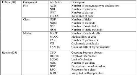
These metrics are based on the abstract syntax tree of each file or package. It includes the type of each node (Annotation type declaration, modifiers…), size of AST and the frequency of nodes in AST. This information can be used to calculate other software metrics without reanalyzing the source code. Eclipse bug data set is publically available on Promise data repository [20]. All experiments are performed on complexity metrics of eclipse data set of version 2.0, 2.1, and 3.0 at package level. Information regarding attributes used in this research work is given in Table 2.
In addition, we used Equinox design metrics. Equinox data set have overall 18 features and 5 bug related attributes which denotes the severity of bugs with the number of occurrences. From the 18 features we select 8 design level metrics which available at the end of design phase of SDLC. Instead of using bug severity level information we use a binary class attribute which only represents buggy or non buggy modules which listed in Table 2.
4.
WORKING METHODOLOGY
The objective of this research is to build an efficient Fuzzy inference system that can learn and predict bugs in software products. Here, we have applied SVM, a supervised training algorithm for classification of data into two sets, buggy and non-buggy. Then various rules are generated inferred from the support vectors. The final set of the rules is chosen from the given set of rules using genetic algorithm optimization. The experiments were performed on Eclipse bug data on package level. Data contains the bugs reported before and after the release of product, called pre and post defects. Using the post defects as class labels for buggy and non buggy, rule base is prepared.
4.1 Performance Measurements
The performance of SVFCS is evaluated through the measures based on confusion matrix. The confusion matrix (also called a contingency table) is a measurement table which relates the
Data set No. of attributes
Class distribution No. of instances
Iris 4 33.33% 150
Diabetes 8 N (65%), P (35%)
768 Eclipse 2.0 199 NB (49%),
B (51%)
377 Eclipse 2.1 199 NB (55%),
B (45%)
434 Eclipse 3.0 199 NB (52%),
B (48%)
661 Equinox 8 NB (60%),
B (40%)
Table 2. Attributes Information.
predicted results with the real values of the dataset, and therefore, it makes possible to obtain measures about the hit and miss of the classifier. For a given model and set of instances, there are four possible outcomes associated with it. If the instance is defective (in fault prediction approach) and it is predicted as defective, it is counted as a true positive; if it is predicted as non-defective, it is counted as a false negative. If the instance is defective and it is predicted as non-defective, it is counted as a true negative; if it is predicted as defective, it is counted as a false positive. This two-by-two confusion matrix, Fig.1, (for binary class problem) forms the basis for many common metrics. The measurements based on confusion matrix include accuracy, precision, recall, and F-measure. In literature these measures are widely used to evaluate the prediction results of a classifier. Next we explained all these measures.
Accuracy
In a binary class problem, accuracy is the ratio of the correctly classified instances to the total number of instances. It measures the hit and miss of the classifier and measures as follows:
Accuracy=
Predicted
Buggy Non-Buggy Original Buggy TP= True Positive
Rate
FN=False Negative Rate
Non-Buggy
FP=False Positive Rate
TN=True Negative Rate
Figure 1. Confusion Matrix.
Precision
It denotes the correctness of the predicted results and measures the miss classification rate. It is defined as the ratio
of the total number of correctly detected instances to the total
number of detected instances for particular class (buggy or non-buggy). It can be calculated as:
Precision=
Recall
The recall measures the ratio of correctly classified instances, for one class (buggy or non-buggy), to the total number of instances that really belongs to the class. It counts the number of hits of the classifier for the class. It is also known as probability of detection and can be calculated as:
Recall=
However, there is a significant trade-off between recall and precision[28,29]. For instance, if model predicts only one module and it belongs to the desired class than the model’s precision will be 1 but, the recall will be low if the desired class contains more than one modules. In contrast, if model predicts all the defective modules correctly along with some non-defective modules incorrectly, it results in high recall and low precision. Therefore, there is a need of a combined measurement strategy such as F-measure, which efficiently combines the recall and precision in a single efficient measure.
F-measure
The F-measure combines the values of precision and recall for a classifier, for one class (faulty or not-faulty). It considers the measurements, recall, and precision, equally important and is calculated by taking their harmonic mean.
F-measure=
ROC
Receiver operating characteristics graph are well known technique for assessing the classifiers performance. It is a two dimensional graph in which abscissa represent the probability
Eclipse[20] Component Attributes Description
File ACD
NOI NOT TLLOC
Number of anonymous type declarations Number of interfaces
Number of classes Total lines of code
Class NOF
NOM NSF NSM
Number of fields Number of methods Number of static fields Number of static methods
Method FOUT
MLOC PAR VG FAN_IN
Number of method calls Method lines of code Number of parameters Cyclomatic complexity
Count of calls of higher modules
Equinox[24] CBO
DEPTH LCOM NOC DOC RFC WMC
Coupling between objects Depth of inheritance Lack of cohesion Number of children
Dependence on a descendent Response for a class
of false alarm or cost and ordinate represent the probability of detection or benefit. It can handle both discrete and continuous classifiers. Discrete classifiers output only the class level, where as continuous classifier output a curve. Each discrete classifier produces a pair of PF and PD that represent a point on ROC graph. Definition of ROC curve contains some interesting points:
(a)
Point (0, 0) denotes that it would never trigger a false alarm and also never issue a positive classification.(b)
Any point situated on the line that is drawn in between (0, 0) to (1, 1) contains no information.(c)
Point (0, 1) denotes the ideal position .But it’s never achieved by any classifier. So any classifier situated close to this point, is always preferable.5.
LEARNERS
This section contains the information regarding the classification and optimization algorithms used in this study. 5.1. SUPPORT VECTOR MACHINE
Support vector machines (SVM) are Kernel based classification approach proposed by Vapanic [25]. It works on the concept of decision planes which defines the decision boundaries between the objects of different classes. Basically SVM is designed for two class problems in which it defines an optimal decision hyperplane based on number of support vectors to classify the data objects however; it can be extended for multiclass problems. Support vectors are the subset of initial data set which is used to define a decision boundary between the classes. Some basic characteristics of SVM are
1. It can be generalized for high dimensional data sets. 2. SVM is formulated as quadratic programming
problem; therefore it provides a global optimal solution.
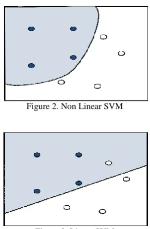
[image:4.595.91.243.518.750.2]3. It is robust to outliers because it uses a margin parameter ∆c to control the misclassification error.
Figure 2. Non Linear SVM
Figure 3. Linear SVM
In the rest of the section we briefly discuss the SVM for both linearly and non- linearly separable data.
5.1.1. LINEAR SVM
For linearly separable data, SVM attempts to draw a decision line (hyperplanes, in high dimension) between two classes in such a way that the distance between the support vectors of two classes and the decision line is maximized. Fig. 2 shows the linear separation of two classes in two dimensional space. Mathematically, for a binary class problem we have to approximate a function ₣: Rd→ {±1} using training data in the
d dimensional space. Let we have two classes C1 and C2
represented as x C1 when y= +1 and x C2 when y= -1; (xi,yi)
Rd × {±1}. For a linearly separable data there exists a pair
of (w, b) such that
C1 (1)
C2 (2)
For all i = (1…….n); where w is the weight vector which represents the vector orthogonal to d dimensional space and b is the bias term. We can recombine the inequality constraints as
C1 C2 (3)
This learning problem can be reformulated as
(4)
Subject to ,
where (xi, yi) to training set and n is the number of
instances. The quadratic optimization theory can be used to solve this problem. The dual form of the above optimization problem is obtained using Lagrangian duality technique which is shown in the following equations:
Maximize (5)
Subject to , and i=1,2,……n.
The solution of this optimization problem is found in the form of vector α =( .An input pattern is classified according to the sign of decision function as
₣ (6)
₣₣
5.1.2. NON-LINEAR SVM
In cases where SVM cannot classify the data objects using liner formulation, it extends its capability by mapping the data objects into the higher dimension feature space using the non-linear mapping, such that x→£(x) where £: Rd→Rs
correspond to the curved surface in lower dimensional space. This transformation can be done using the Kernel function which is defined as:
K ( )= £ £ (7) Therefore, the optimization problem of linearly separable case, equation 5, can be reformulated to handle the non linear data objects as:
Maximize (8)
Subject to ,
and i = 1,2,……n (9) where K( ) is the kernel function which is used for nonlinear mapping of the data objects into the high dimensional feature space. The classification decision can be constructed as
₣ (10)
₣₣ (11)
The most common kernel functions used in literature are Linear: K( )= .
Polynomial: K( )= d
Gaussian (RBF) K( )=
Sigmoid (MLP) K( )=tanh(
We have tried all the three nonlinear kernel functions for our experiments. The Gaussian (RBF) yielded the best performance result, therefore we have used RBF kernel for further experiments
.
5.2 NAIVE BAYES
Naïve Bayes (NB) [28] classifier is the statistical classifier which uses the Bayes posterior probability theorem. The primary axiom of NB classifier is “All attributes are uncorrelated”. Posterior probability of each class (defective or non defective) is calculated on each attribute of each data instance and data is assigned to class with the highest posterior probability. It can handle both continuous as well as discrete attributes efficiently. For a given dataset of size D with N attributes and M classes NB classifier computes the posterior probability for vector X by equation 12 and assigns X to the class for which it possess maximum posterior probability.
(12)
For continuous attributes (13) and (14) are used.
(13)
(14)
Here C is the class variable, X is a random vector which represents attribute values and represents the mean and the standard deviation of the attributes.
5.3 FUZZY INFERENCE SYSTEM
Fuzzy inference is the process of mapping from given input to an output using fuzzy logic. Mapping provides the information regarding decision making. Several methods have been used for fuzzy classification [22]. For n training patterns (X11……..Xnm) with m features and C classes we can inferred
fuzzy if then rules using support vectors as given below. Rule : If X1 is A11 and … and Xm is A2m then class of X = Ci
Where Xj is jth feature of the input X, and each of Aij
represents membership grade with Gaussian membership function with center Vij and standard deviation one.
Membership of Xj is defined as
(15)
To calculate the firing strength of each rule we used product operation between each antecedent for given input pattern and classification decision is made according to the rule which have maximum firing strength. Firing strength of Vi (vector i)
for input X is
(16)
For this study we inferred “Sugeno type zero” fuzzy rules in which consequent part is constant (defective or non-defective). For a training patterns (support vector) (X11……..Xnm) with m features and c classes we can construct
fuzzy if then rules as given below for classification. Rule : If X1 is A11 and … and Xm is A2m then class of X = Ci
An example of fuzzy expert system is presented in Fig. 4.
5.4 GENETIC ALGORITHM
Genetic algorithm [29] is the process of global search and optimization, modeled from natural genetics inspired by the biological evolution process, which explore the search space by incorporating a set of candidate solution in parallel, Fig. 5. It maintained a set of candidate solution and evolves it by applying a set of stochastic operations. Stochastic operations are:
Reproduction: - Reuse the existing solution by copying it into the new population with the reproduction probability.
Crossover: - New solutions are generated by recombining the randomly selected part of the selected solution on the basis of crossover probability.
5.4.1 GENETIC REPRESENTATION AND FITNESS EVOLUTION
In this work a chromosome is represented by a rule vector as V = (v1 v2 ... vn), where n is the number of the fuzzy rules
which are generated and Vk is the boolean value representing
whether the k’th rule is selected in the rule vector V or not. Vk={0 if rule is not selected and 1 if rule is selected}. Each
rule vector V is obtained by randomly assigning 1 or 0 to each parameter of V. The length of V is same as number of rules. Consider the set of Chromosomes V = (v1 v2 ... vn). The
fitness score of the rule vector is determined by [27]: Eval (Vt) = w1・f1(Vt) − w2・f2(Vt), (16)
Where w1 and w2 are non-negative constant weights assigned
to the two kinds of objectives, f1 (Vt) is the classification
performance determined by the measurements (accuracy, recall and precision) and f2(Vt) is the number of the fuzzy
rules in fuzzy rule set.
6.
MODEL GENERATION
Our prediction model is generated through three phases. Initially, the first set of IF-THEN rules is obtained through an equivalence of the SVM training. Attribute values of each support vectors combined with AND (connective) treated as antecedent part and class value work as consequent part of the rule; which is further used for classification. The second set of rules is generated by combining the first set based on strength of firing signals of support vectors using Gaussian kernel. The main advantage of this method is that, it guarantees that the number of final fuzzy IF THEN rules is not more than the number of support vectors in the trained SVM. Genetic algorithm is applied for rule set optimization which simultaneously enhances or maintains the performance of the model and minimizing the number of rules used for classification. In other words, the optimization is performed while considering both the minimization of the number of the extracted fuzzy rules and the maximization of the performance of the fuzzy classification system, i.e., the number of correctly classified training patterns with the less fuzzy rules. Basically the model work as zero order Sugeno type fuzzy inference system [22]. Basic steps of model generation are:
1. Data sampling is done using stratified sampling. Partition the selected data set in training and testing set maintaining the same ratio of both classes in each set. 2. Normalize the test and train dataset such that they have
zero mean and unit variance.
3. Perform SVM classification on training data set using the box constraint value as per number of rules desired and ‘RBF’ kernel function.
4. Construct the if then else rule for each support vector like Rule Rq: If X1 is Vq1 and … and Xm is Vqm then class of
X = Class of V.
5. Calculate the membership degree of each feature of a data point using Gaussian membership function.
6. Calculate the firing strength for each rule using multiplication T-norm operation.
7. Assess the performance of rule set using accuracy, precision, and recall.
8. Apply Genetic algorithm for rule set optimization by using fitness evolution function.
Block diagram of model generation process is shown in Fig.6.
7.
RESULT AND DISCUSSION
Experiments were conducted by splitting the overall data set into training with 67% and testing with 33%. We repeated our experiments 10 times and randomize the input each time. This repletion is required to mitigate the impact of order effect. Results of experiments are given in Table 3 and 4 which contain the Recall (PD), Precision, Probability of false alarm (PF), Accuracy, and F-score of experiments on different data sets. We compare our results with two other model based on two well known classifiers NB and SVM. Iris and Pima Indians Diabetes data set are used for model validation. On iris data set our model gives 100% recall (Probability of detection also denoted as PD) and 0% false alarm rate (PF) with 100% accuracy where as on Pima Indians Diabetes data set it gives 68.6% and 29.5% PD and PF respectively which is better than previous known result (60% and 19%[23]) except in PF which should be low. Validation results using these two datasets suggest that we can use this model in software defect prediction.
Figure 4. Fuzzy Expert System.
Figure 5. Rule Set Optimization Using Genetic Algorithm.
Figure 6. Defect Prediction Model Generation.
Input
Data Fuzzyfication
Knowledgebase
Fuzzy Inference Engine Defuzzyfication Feedback
Initial
Rule Set
Best Offspring
Selection Discard Remaining Rule Sets Population
Generation
Performance Assessment of Rule Sets Rule Set Modification Using GA
Operators Selection
Defect Database
Data Sampling Data
Normalization
SVM Training
Support Vector Extraction Fuzzy IF THEN
Rule Generation Using Gaussian
Function GA Based
Optimization
Rule Testing and
Performance Assessment Fuzzy
Rulebase Fitness Criteria is Satisfied
Table 3. Results on Validation Data.
Table 4. Classification Results of Eclipse and Equinox Data Sets
SVM 71.5 89.7 39.7 2.4 55.5 No
Eclipse 3.0
SVFCS 70.4 66.8 76.4 34.2 50.2 18.1
NB 68.1 82.3 40.8 7.8 54.4 No
SVM 68.2 81.7 40.3 8.2 53.1 No
Equinox SVFCS 68.5 56.5 77.7 38.7 43.1 11.9
NB 72.1 80.8 39.6 6.3 54.9 No
SVM 73.2 75 47.7 10.1 57.5 No
8.
CONCLUSION AND FUTURE
DIRECTIONS
In this paper a novel approach, SVFCS, for fault prediction is presented. SVM, FIS, and Genetic algorithm are well known methods and are used for classification in every branch of engineering and science. In this work first time we combined the advantages of these three learners to get better prediction model. Performance of the model is checked against the open source data project where as in previous studies [10] assessment has been done on historical data sets which are publically available but could not ease the testing task in real development due to technology changes. The result of SVFIS is confronted with other two well-known algorithms used in the fault-proneness problem. The experimental results reveal the effectiveness of SVFIS in fault prone module prediction, and endorse that it can be useful and practical addition to the framework of software quality prediction. Moreover, the superior performance of SVFIS, especially in recall of faulty modules, can have a practical implication in the context of software testing by mitigating the risks of miss detection of fault prone in early stage of development. By using this model we extract more knowledge and ease the testing task in early phase of software development life cycle.
This study need to be extended for validation purpose. Initially it works on binary classification problem we plan to generalize this model for multi class problem. We also plan to investigate the impact of support vectors on other classifier’s performances.
9.
ACKNOWLEDGMENTS
[image:8.595.289.529.119.518.2]The authors gratefully acknowledge the valuable comments by the anonymous reviewers. These comments have greatly helped in improving the quality of the revised paper.
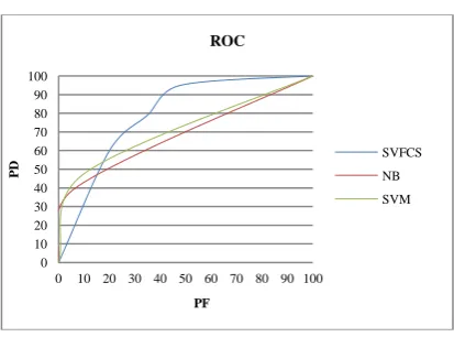
Figure 7. ROC Graph for Eclipse 2.0.
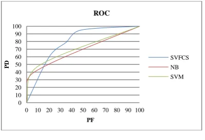
Figure 8. ROC Graph for Eclipse 2.1.
0 10 20 30 40 50 60 70 80 90 100
0 10 20 30 40 50 60 70 80 90 100
PD
PF
ROC
SVFCS
NB
SVM
0 10 20 30 40 50 60 70 80 90 100
0 10 20 30 40 50 60 70 80 90 100
PD
PF
ROC
SVFCS
NB
SVM
Data Set Accuracy Precision Recall Probability of False alarm
F-Score Number of Rules Eclipse
2.0
SVFCS 72.5 70.5 78.6 34.2 55.3 11.9
NB 66 83.8 39.8 7.35 53.9 No
SVM 68.9 84.8 46.3 8.1 60.2 No
Eclipse 2.1
SVFCS 70 66.2 73.3 31.5 48.6 16
[image:8.595.325.532.527.680.2]Figure 9. ROC Graph for Eclipse 3.0.
Figure 10. ROC Graph for Equinox.
10.
REFERENCES
[1] Tian, J., “Software Quality Engineering: Testing, Quality Assurance, and Quantifiable Improvement” John Wiley & Sons, (2005).
[2] Laprie, J.C., and Kanoon, K.,” Software Reliability and System Reliability, Handbook of Software Reliability Engineering”. M.R. Lyu, 1,27-69, IEEE CS Press-McGraw Hill, (1996).
[3] Emam, K.,El., “The ROI from Software Quality”. Auerbach Publications, Taylor and Francis Group, LLC, (2005).
[4] Khoshgoftaar, T.M., Allen, E.B., Kalaichelvan, K.S., Goel, N., “Early Quality Prediction: A Case Studv in Telecommunications”. 2006, IEEE Software.
[5] http://www.softwaretestingtimes.com/2010/04/softwarete sting- effort-estimation.htm.
[6] Khosgoftaar, T.M., Munson, J.C.,”Predicting Software Development Errors Using Software Complexity Metrics”. IEEE Journal On Selected Areas In Communications1990, 8(2).
[7] Yuan, X., Khoshgoftaar, T.M., Allen, E.B., Ganesan, K., “ An Application of Fuzzy Clustering to Software Quality Prediction.2000 In: Proceedings of The 3rd IEEE Symposium on Application-Specific Systems and Software Engineering Technology
[8] Jiang, Y., Cukic, B., Menzies, T.,”Fault Prediction Using Early Lifecycle Data”. 2007 In: Proceedings of ISSRE , TBF
[9] Basili, V., R., Briand, L., C., Melo, W., L, “ A validation of object-oriented design metrics as quality indicators”.1996, IEEE Trans. on Software Engineering. 22, 751-761.
[10]Menzies, T., Greenwald, J., Frank, A., “Data Mining Static Code Attributes to Learn Defect Predictors.” 2007 IEEE Trans. Software Eng. 33, 2-13.
[11]Subramanyam, R., Krishnan, M.,S., “Empirical analysis of ck metrics for object-oriented design complexity: Implications for software defects”.(2003) IEEE Trans. Software Eng.29, 297-310.
[12]Binkley, A., B., Schach, S., R., “Validation of the coupling dependency metric as a predictor of run-time failures and maintenance measures”.1998 In: International Conference on Software Engineering, pp. 452-455.
[13]Schröter, A., Zimmermann, T., Zeller, A., “Predicting failure-prone components at design time”.2006, In: 5th International Symposium on Empirical Software, Rio de Janeiro, Brazil,
[14]Nagappan, N., Ball, T. “Explaining failures using software dependences and churn Metrics”. 2006,Microsoft Research, Redmond, WA.
[15]Xing, F., Guo, P., Lyu, M. R. “A Novel Method for Early Software Quality Prediction Based on Support Vector Machine”.2005,In: Proceedings of The 16th IEEE International Symposium on Software Reliability Engineering
[16]Jiang, Y., Cukic, B., Menzies, T., Bartlow, N., “Comparing Design and Code Metrics for Software Quality Prediction”2008. In: PROMISE 2008, ACM, New York
[17]Yang, B., Yao, L., Huang, H.Z., “Early Software Quality Prediction Based on a Fuzzy Neural Network Model”.2007, In: Proceedings of Third International Conference on Natural Computation.
[18]Quah, T.S., Thwin, M.M.T. “Application of Neural Network for Predicting Software Development Faults Using Object-Oriented Design Metrics”.2003,In: 19th International Conference on Software Maintenance. IEEE Computer Society, Los Alamitos.
[19]Wang, Q., Yu, B., Zhu, J. “Extract Rules from Software Quality Prediction Model Based on Neural Network”.2004, In: Proceedings of The 16th IEEE International Conference on Tools with Artificial Intelligence, ICTAI
[20]Promise. http://promisedata.org/repository/.
[21]Zimmermann, T., Premraj, R., Zeller, A., “Predicting Defects for Eclipse”.2007, In: Third International Workshop on Predictor Models in Software Engineering. Promise.
[22]Pitiranggon, P., Beenjathepanun, N., Banditvilai, S., Boonjing,V. “Fuzzy Rule Generation and Extraction from Support Vector Machine based on Kernel Function Firing Signal”.2010, International journal of Engineering and applied sciences. 6,244-251
[23]UCI machine learning http://archive.ics.uci.edu/ml/. [24]Bug Prediction data set http://bug.inf.usi.ch/.
[25]Fawcett, T., “ROC Graph: Notes and Practial Consideration for Data Mining Researches”. 2003 Intelligent Enterprise Technology Laboratory.
[26]Vapnik,V. “The nature of Statistical learning theory”. 1995,Springer, New York
[27]Burges, C.,”A tutorial on support vector machines for pattern recognition”.1998 Data mining and knowledge discovery 2,121-167.
[28]Witten I., andFrank E. “Data mining”. 2nd edition. Los Altos, US: Morgan Kaufmann, (2005).
[29]Koru A .G, Liu H. “An Investigation of the Effect of Module Size on Defect Prediction Using Static Measures.” Proc. Workshop Predictor Models in Software Engg, (2005).
0 10 20 30 40 50 60 70 80 90 100
0 10 20 30 40 50 60 70 80 90 100
PD
PF
ROC
SVFCS
NB
SVM
0 10 20 30 40 50 60 70 80 90 100
0 10 20 30 40 50 60 70 80 90 100
PD
PF
ROC
SVFCS
NB