Analysis of Adaptive Semiblind Channel Estimation Scheme with Missed Data Channel Estimation Schemes in MIMO Antenna system

Analysis of Adaptive Semiblind Channel Estimation

Scheme with Missed Data Channel

Estimation Schemes in MIMO Antenna System

Ravi Kumar, Rajiv Saxena

Department of Electronics & Communication Engineering,

Jaypee University of Engineering & Technology, A.B.Road, Raghogarh, Guna.(M.P.), India.

ABSTRACT

Multiple Input Multiple Output (MIMO) antenna systems are being given much attention to provide high capacity with less bandwidth requirement. In this paper, some channel estimation techniques have been tried to implement with the adaptive semiblind channel estimation scheme using less requirement of pilot symbols similar to as in the case of the estimating the channel with known channel state information(CSI) conditions with requirement of high channel bandwidth which is not required in this analysis. The improved results have been found with less requirement of channel bandwidth and compared with the already simulated results. It is shown that in addition to improving the spectral efficiency, the proposed technique offer better semiblind channel estimation accuracy for the partial CSI conditions.

Keywords

Semiblind MIMO Channel Estimation, MIMO Antenna System, Partial CSI, Blind Channel Estimation.

1. INTRODUCTION

MIMO Antenna system is widely used technique for high data rate transmission over frequency-selective fading channels due to its capability to combat the inter-symbol interference (ISI), low complexity, and spectral efficiency nowadays[1]. Even rich scattering environment is the key support for the MIMO technology at both the transmitter and receiver ends which results in further increase in the capacity[2]. SPACE-TIME coding is a powerful means to exploit spatial diversity and to combat fading in multiple-input multiple- output (MIMO) wireless communication systems. The data rate may be enhanced by using spatial multiplexing in MIMO systems, whereas the reliability may be enhanced by using space time coding (STC). Various space time codes have been developed till the date but orthogonal space–time block codes (OSTBCs) [3] are of particular interest because they achieve full diversity while offering very simple maximum-likelihood (ML) decoding in the single-user case.

Self interference problems created by MIMO systems have been resolved by various algorithms i.e. STBC[3, 4], SVD [5], VBLAST [6] and so on. They fall into two main categories: spatial multiplexing-based algorithms [5, 6] and diversity-based algorithms[3, 4] . Spatial multiplexing is highly spectral efficient: it takes advantage of spatial diversity of MIMO channels and creates parallel sub-channels over which separate data streams can be transmitted; while diversity-based algorithms, e.g. STBC, aims to build up a reliable wireless link with high diversity order. These algorithms have different performance in terms of capacity[7]; and even within the same algorithm, the performance varies randomly under different channel conditions. Therefore, in adaptive systems to

achieve the maximal spectral efficiency, we need to know the channel state information at the transmitter to adjust the transmitter accordingly, i.e., the algorithm, the modulation order and even the power and the coding rate[8, 9].

In most of the estimation techniques, it is known that the CSI of the transmitters is available at the receiver. This implies that pilot symbol should be used to estimate the transmitter CSI. Whereas it is known that, use of pilot symbol may reduce the spectral efficiency and therefore blind and semiblind techniques can be used for spatial channel model with partial CSI knowledge.

Among the parameters to adapt at the transmitter, the work has been confined to find the optimal algorithm associated with the possible maximal constellation size. To be able to select the optimal algorithm under certain channel conditions, we need to know accurately beforehand the spectral efficiency of the algorithms at different signal to noise ratio (SNR) which has been shown in [10]. Although several theoretical upper bounds[11] of the spectral efficiency have been suggested, e.g. capacity, continuous-rate spectral efficiency, they are not accurate enough to be the metric on which the adaptation scheme is based.

In general, data dependant (or data adaptive) filters outperforms their data independents counterparts and are preferred in many applications. A well know adaptive filter bank method is CAPON spectral estimator which has been simulated in [12] and the satisfactory results were found as compared with the existing results. Li and Stoica [13] gave another adaptive filter bank method with enhanced performance as compared with the CAPON estimator, which is referred as the Amplitude and Phase estimation (APES) and Gapped-data APES (GAPES). These estimators have been tried in this paper for implementing with the APASBCE scheme for making the system more stable and less complex. When the measurements during certain periods are not valid due to many reasons such as interferences or jamming, in APES, samples can occur at arbitrary places among complete data set, whereas in GAPES, missing samples may occur in groups of available data samples where within each group there are no missing samples.

These APES and GAPES estimation schemes are used with utilizing the proposed Adaptive Pilot Assistant Semi-Blind Channel Estimation (APASBCE) scheme which shows some improved results. These results have been compared with the existing results available in the literature and with each other. A new approach of closed-form expressions of the spectral efficiency, coined as discrete-rate spectral efficiency, as a function of SNR has been derived which is shown to be a very precise estimation to be applied in adaptation.

the optimal algorithm can be found as long as the SNR is given. The remainder of this paper is organized as follows.

2. SYSTEM MODEL

A MIMO-OFDM system has been considered with T M transmit antenna &

M

_R receive antenna, which communicates over a flat fading channels, and is abbreviated as M_TM_R receive MIMO systems matrix H. The system is described by y k( )Hx k( )n k( ), where x is

1( ),. ( ),....2 T( ) T

M

x k x k x k

 

  which is the transmitted symbol

vector of

M

_T transmitter with the symbol energy given by

2 2 | _m( ) |

E_ x k  _



for

1

 

m

M

T and covariance matrix ( H)

QE XX , y denotes the received vector

1( ), 2( ),... R( )

T M

y y k y k y k _ and ( ) 1( ), 2( ),.... R( )

T M n k  n k n k n k_ is

the complex valued gaussian white noise vector at the receiving end for MIMO channels with energy

2 ( ) ( ) 2

R

H

n M

E n k n_ k  _



I distributed according to Nc 2

(0,

)

R

n

I

M



assumed to be zero mean, spatially & temporally white and independent of both channel & data fades. The channel model considered here denoted by 1/2 1/2

R T

HR H R

[14] with R_T&R_Rrepresenting the normalized transmit and receive correlation matrices with identity matrix. The entries

of

H

_are independent and identically distributed (i.i.d.)

Nc(0,1). Here the CSIR is described by

1/2 1/2 1/2 1/2

ˆ

_,

ˆ

_,

R T R T

H



H



E

H



R H R

_

E



R E R

_

(1)

where

H

ˆ

is the estimate of H & E is the overall channel estimation error matrix,

H

ˆ &

_

E

_are white matrices spatially uncorrelated with i.i.d. entries distributed according

to Nc (0,1-2

E



) & Nc(0, 2

E



) with variance



_E2 of channel estimation error.[15].

If it is assumed that the system is having lossless feedback i.e. CSIT & CSIR both are same. Thus

H R R

ˆ , , , &

_{R T}



_E2



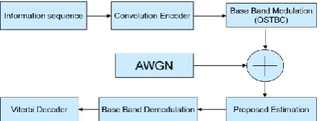
_n2 represents that the CSI is known to both the ends. With the partial CSI model, the channel output can be considered as

ˆ

[image:2.595.56.289.582.670.2]

y



Hx



Ex



n

. The system model with proposed estimation scheme has been shown in Figure 1.

Figure 1. System Model with Proposed Estimation schemes

3. PROPOSED METHOD TO

IMPLEMENT THE SEMIBLIND

CHANNEL ESTIMATION APPROACH

USING APASBCE

Now considering the problem of estimating the amplitude spectrum of a complex valued uniformly sampled

discrete-time signal

{ }

y

_{n n}N_₀1. For a frequency



of interest, the signal

y

_n is modeled as

( ) j n ( ) 0,... 1, (0 2 )

n n

y  e e  n N    (2)

where, α(ω) denotes the complex amplitude of the sinusoidal component at frequency ω, and en(ω) denotes the

residual term i.e. zero mean noise and interferences from frequencies other than ω. The problem of interest is to estimate α(ω) from signal for any given frequency ω.

Let h(ω) denote the impulse response of an M-tap finite impulse response(FIR) channel response,

( ) [ ₀( ) ₁( ) ... ₁( )]T

h h  h  _hM  (3)

Where,

( )

T

denotes the transpose. Then the receiver output

can be written as H

( )

ˆ

l

h



y

, where,

1 1 1

ˆ [

l l l M

] ,

T

0,

,

1

y



y y





y

 

l



 

L

(4) These are the Mx1 forward data sub vectors and L=N-M+1. For each ω of interest, we consider the following design objective,

1 ₂

ˆ

min | ( ) ( ) | . . ( ) ( ) 1

( ), ( ) 0

L _{j l H}

H

h y_l e s t h a h l



    

  



  

 (5)

Where, a(ω) is an Mx1 vector given by,

 1

( )

[ 1

j

.

j M

]

T

a





e





e

  (6)

The channel coefficient h(ω) is designed such that the channel sequence is as close to a sinusoidal signal as possible in a least squares(LS) sense and the complex spectrum α(ω) is not distorted by the filtering.

Let g(ω) denote the normalized Fourier transform of

y

ˆ

_l,

1

0

1 ˆ

( )

L

j l l l

g y e

L



  







(7)

And define,

1 0 1

ˆ L _{ˆ ˆ}H l l l

R y y

L

 





(8)

Equation (5) can be written as,

2

ˆ

( ) ( ) *( ) ( ) ( ) ( ) ( ) | ( ) |

H H H

h  Rh  h  g   g h  

   

2

ˆ

2

| ( )

 

h

H

( ) ( ) |

 

g

h

H

( )



Rh

( ) |



h

H

( ) ( ) |

 

g









(9)

where,

( ) *

denotes the complex conjugate.

The minimization of (9) w.r.t.

 

( )

is given by,

ˆ( )

h

H

( ) ( )

g

 



 

(10)

By putting (10) in (9), yields the following minimization problem for the determination of h(ω),

( )

ˆ

min H( ) ( ) ( ) . . H( ) ( ) 1

h h  S h s t h  a  ₍₁₁₎

where,

ˆ_{( )} ˆ _{( )} H_{( )}

S R g g  (12)

The solution of (11) is obtained from [16] as

1 1

ˆ ( ) ( ) ˆ( )

ˆ

( ) ( ) ( ) H

S a

h

a S a

  

  





This is the forward only APES channel coefficients, and the forward only APES estimator in (10) becomes,

1 1

ˆ

( )

( ) ( )

ˆ( )

_ˆ

( )

( ) ( )

H

H

a

S

g

a

S

a







 



 

 



(14)

3.1 Forward Backward Averaging

Here we consider the data for the conditions when received data appeared at the receiver from multiple directions due to diversity effect. Let the backward data subvectors be constructed as

* * *

1 2

[

...

] ,

T

0,...,

1

l N l N l N l M

y



y

_{ }

y

_{ }

y

_{ }

l



L



(15) The outputs obtained by running the data through the channel both forward and backward are as close as possible to a sinusoid with frequency ω. This design objective can be written as 1 2 ( ), ( ), ( ) 0 2 1 _ˆ

min {| ( ) ( ) | ...

2

| ( ) ( ) | } . . ( ) ( ) 1

L

H j l

l h

l

H j l H

l

h y e

L

h y e s t h a

                    



(16)

The minimization of (16) w.r.t.

 

( )

and

 

( )

gives

ˆ( )

h

H

( ) ( )

g

 



 

and

 

ˆ( )



h

H

( ) ( )



g



, where

( )

g



is the normalized Fourier transform of

y

ˆ

_l,

1 0 1 _ˆ ( ) L j l l l

g y e

L





 







(17)

It follows that (16) lead to,

( ) ˆ

min H( ) ( ) ( ) . . H( ) ( ) 1

fb

h h



S

 

h s t h

 

a 

(18)

where,

( ) ( ) ( ) ( )

ˆ _{( )} ˆ

2

H H

fb fb

g g g g

S  R       (19)

with, 1

0 1 ˆ L _{ˆ ˆ}H

f l l

l

R y y

L

 





, 1

0 1 ˆ L _{ˆ ˆ}H

b l l

l

R y y

L

 





for forward and backward received signals, and,

ˆ ˆ 2

f b

fb

R R R  

The solution for (18) is given by,

1 1

ˆ _{( ) ( )}

ˆ ( ) _ˆ

( ) ( ) ( ) fb fb H fb S a h

a S a

         (20)

Because of readily verified relationship, we have ( ) H( ) [ ( ) H( )]T

g g  J g g  J (21)

where,

J

denotes the exchange matrix whose non-diagonal elements are ones and the remaining elements are zeros. So

fb

S

can be conveniently calculated as

ˆ

_{( )}

ˆ

_{( )}

ˆ ( )

2

T

f f

fb

S

JS

J

S











(22)

where,

ˆ _{( )} ˆ _{( )} H_{( )}

f f

S



R g



g



(23)

Given the forward Backward APES based channel coefficients

h

_fb

( )



, the forward-backward spectral estimator can be written as

1 1 ˆ

( ) ( ) ( )

ˆ ( ) _ˆ

( ) ( ) ( )

H fb

fb H

fb

a S g

a S a







 



 

   (24)

due to this relation, the forward backward estimator can be simplified as,

* ( 1)

ˆ

_{( )}

H

_{( ) ( )}

_ˆ

jw N

fb

h

fb

g

fb

e

 

_





_



 

(25)

It indicates that from

 

ˆ ( )

_fb , we will get the same forward

backward symbol estimator

 

_fb

( )

.

These are comparable with (13) and (14) which are generally better estimates of the true R and

Q

( )



ideal covariance matrices with and without presence of the signal of strength. For implementing the algorithm for fast processing and to avoid the inversion of matrix which is the drawback in estimating the semiblind channel can be reduced by using Cholesky factorization method for covariance matrices.

3.2 GAPES based channel estimation

This algorithm states two separate conditions i.e. estimating the channel adaptively with finding out the corresponding channel coefficients and then filling the gapped sequences in between the received data adaptively implementing the APASBCE scheme in it. Assuming some segment of data signals are unavailable. Let a complete data vector y, whose length are N1,…..Np, respectively, with N1+N2+….+Np=N,

1 2 1

1 2

[ ... ]

[ ... ]

T N

T T T T

p

y y y y

y y y



 

(26)

A gapped data vector



is formed by assuming yp, for p = 1,3, …P (P is always an odd number), are available,

1 3

[

y

T

y

T

....

y

T TP

]



(27)

2 4 1

[

T T

....

T

]

T P

y

y

y



_ (28)

where



denotes all the missing symbols. Then



and



have dimensions gx1 and (N-g)x1, respectively, where g= N1+N3+….+Np is the total number of available symbols. Now

it is required to estimate the initial amplitude and phase estimates of

h

( )



and

 

( )

from the available data



. Choosing initial channel length

M

₀ such that an initial full rank covariance matrix R can be built with the channel length

0

M

, using only the available data segments. This indicates

0 0

{1,3,... }

max(0, _p 1)

p P

N M M



  



(29)

Let Lp=Np-M0+1 and let J be the subset of {1,3,…P} for

which Lp>0. Then the channel coefficients h(ω) is calculated

from (12) and (13) by using

1 1 1

1 1

....

....

1

ˆ

p p

p

N N L H l l P J l N N p

P J

R

y y

L

          









(30)

1 1 1

1 1 .... ....

1

( )

p p p

N N L

j l l p J l N N p

p J

g

y e

L





           









(31)

Data subvectors above have a size of M0x1 whose elements

Now the channel coefficients

h

( )



is applied to the available data



abd LS estimate of

 

( )

from the coefficients output

is calculated by using (10), where

g

( )



is replaced by (31). Using this process, only the available symbols are passed through. The initial LS estimate of

 

( )

is based on these so obtained received and filtered outputs only.

Now consider the estimate of μ based on the initial spectral estimates α(ω) and h(ω). Theμ is obtained as the solution by getting



under the condition that the output of the filter h(ω) fed with the complete data sequence made from



, and μ as

close as possible(in LS sense) to

 

( )_ej l

for l = 0,…., L-1.

1 1

2 0 0

ˆ

ˆ

min

|

(

)

(

)

k

|

K L

ej l H

k l k

k l

h

y







 

   





(32)

By estimating



in this way, the system remains in the LS fitting framework of APES estimation technique. By solving the quadratic minimization problem(32), the minimization received w.r.t.



,

1 1

0 0

ˆ ( ) ( ) 1 ( ) ( )

K K

H H

k k k k

k k

B B B d

      

 

   

_{ } _{ }





 





(33)

Once an estimate



has become available, the next step consist of re-estimating the spectrum and the filter bank, by applying APES estimation scheme to the data sequence made from Υ and μ. This leads the minimization w.r.t.

h

(



k

)

and

(

k

)

a



of the function

1 1

2

0 0

ˆ

|

(

)

(

)

k

|

K L

ej l H

k l k

k l

h



y

 



 

 





(34)

subject tohH(



_k) (a



_k)1, where,

y

_lis made from



and



. Evidently the minimization of (34) w.r.t

1 1

2 0 0

ˆ

|

(

)

(

)

k

|

K L

ej l H

k l k

k l

h



y

 



   





, can be decoupled into K

minimization problems of the form of (5), yet it is preferred to

write the criterion as in

h

ˆ ( ) ( ) 1

H

 

a



, to make the connection with (34). This comparison shows that the alternating estimation of



 

(

_k

), (

h



_k

)



and



can be recognized as the cyclic optimization approach for solving the following minimization problem,

1 1

2 ,{ ( ), ( )}

0 0

ˆ

min

|

(

)

(

)

|

. .

(

) (

)

1

k

k k

K L

ej l H

k l k

h k l

H

k k

h

y

s t

h

a



   



 





 

 







(35)

Finally, this minimized value is used with the proposed APASBCE algorithm[17] for finding the value of unknown



and



. Use the most recent estimate of



 

(

_k

), (

h



_k

)



in (35) to estimate



by minimizing the so obtained cost function, whose solution is given by (33). Use the latest estimate of



to fill in the missing data symbols and estimate

1 0

{ (

h

  

k

), (

k

)}

kK



 by minimizing the cost function in (35)

based on the interpolated data. Repeating this whole process for more number of iterations will converge the estimated symbols to the nearly approachable symbol. The practical convergence can be decided when the relative change of the cost function in (35) corresponding to the current and

previous estimates is smaller than a pre-assigned threshold.(e.g.ε=10-3_{). After convergence, final spectral}

estimate are the practical approachable values. The comparison of the proposed approach with the existing estimation method for the MIMO antenna systems has been shown in Table 1.

Table 1. Comparison of different Semiblind Channel Estimation Schemes for their Robustness and Complexity S.No. Name of

Algorithm Filter Based

Robustness Complexity Adaptiveness

1. CAPON Yes Moderate High No

2. MUSIC No Highly Very High No

3. APES Yes High Less Yes

4. GAPES Yes High Less Yes

4. Results

The results will be obtained by putting the values of estimated



to calculate the branch metric 2(M+N-1). Then calculating the tracking ability of the algorithm, if found suitable then the simulation will be terminated otherwise, the M samples from the L samples of information block will be processed again for ktimes. Now again calculating the branch metric as said above, if found suitable this time, calculating the path metric

for all possible paths from the estimated values in

H

ˆ

. Now choosing the path metric with minimum path metric gain



_{i L,} , which will help to track the bits through the chosen path or optimum path. If in case, the channel drops or the fading occur for the estimated channel then, again the algorithm will process for the ksteps. Then taking the short time average value of the detected sequence found in previous step for

. k Jk k

[image:4.595.319.542.484.653.2]

   with minimum value will give us the desired result.

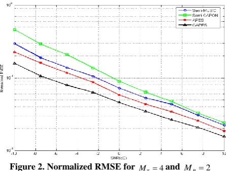
Figure 2. Normalized RMSE for MT 4and MR2 Figure 2. and Figure 3. shows the Normalized RMSE comparison for 4x2 and 4x4 antenna systems for APES and GAPES based semiblind channel estimation schemes with the existing results of CAPON and MUSIC based semiblind channel estimation schemes which shows the improved results as shown. These schemes show better results due to less complexity at the estimation stage.

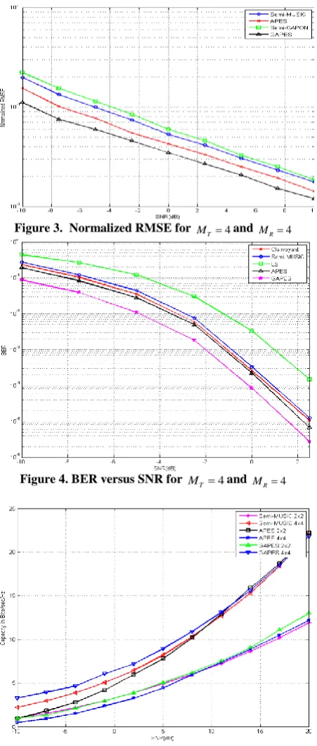
MUSIC based Semiblind channel estimation scheme. The GAPES based semiblind channel estimation scheme maintains the 0.5dB gain throughout as compared with the APES based semiblind channel scheme. Similarly, Figure 5, shows the capacity result comparison of MUSIC based semiblind channel estimation with the APES and GAPES based semiblind channel estimation scheme. It is shown that GAPES based semiblind channel estimation scheme start to show better performance after the SNR level of 12dB and 18db for 2x2 and 4x4 MIMO Antenna systems respectively.

Figure 3. Normalized RMSE for MT4and MR4

[image:5.595.57.283.178.710.2]

Figure 4. BER versus SNR for M_T 4and MR4

Figure 5. Capacity for 2x2 and 4x4 antenna configurations using different Channel Estimation Schemes

5. CONCLUSION

The APES and GAPES based channel estimation scheme has been implemented with APASBCE scheme which shows that there is improvement in the results of the semiblind channel estimation using these filter based estimation schemes. The comparative results shown that the highly complex channel estimation schemes can be replaced using these filter based schemes with the proposed APASBCE scheme. The simulation time was less for the APASBCE based APES and GAPES semiblind channel estimation schemes and moreover the adaptive natures of these filter based schemes are very easy to implement. These schemes can be implemented in mobile environment and in such urban areas where the diversity effect is more common and there is more number of chances of signal fading due to large number of restrictions in between the path of the signal transmitting from one end to the second end of the mobile receiver. These schemes can be expanded to the multiuser MIMO systems where there are more number of data loss due to interference and fading.

6. ACKNOWLEDGEMENT

The author thankfully acknowledges the support provided by the authorities and management of Jaypee University of Engineering & Technology, Guna, India.

7. REFERENCES

[1] R. Kumar and R. Saxena, "Analysis of MIMO capacity for spatial channel model with partial CSI knowledge," in Wireless Communication and Sensor Networks( WCSN), 2008, pp. 187-191.

[2] G. J. Foschini and M. J. Gans, "On limits of wireless communications in a fading environment when using multiple antennas," Wireless Personal Communications, vol. 6, pp. 311-335, 1998.

[3] V. Tarokh, H. Jafarkhani, and A. R. Calderbank, "Space-time block codes from orthogonal designs," Information Theory, IEEE Transactions on, vol. 45, pp. 1456-1467, 1999.

[4] S. M. Alamouti, "A simple transmit diversity technique for wireless communications," Selected Areas in Communications, IEEE Journal on, vol. 16, pp. 1451-1458, 1998.

[5] G. G. Raleigh and J. M. Cioffi, "Spatio-temporal coding for wireless communication," IEEE Trans. Commun., vol. 46, pp. 357–366, Mar.1998.

[6] G. J. Foschini, "Layered space-time architecture for wireless communication in a fading environment when using multi-element antennas," Bell Labs Technical Journal, vol. 1, pp. 41-59, 1996.

[7] D.Tse and P.Vishwanath, Eds., Fundamentals of Wireless communications. Cambridge, U.K.: Cambridge University Press., 2005, p.^pp. Pages.

[8] X. Pengfei, Z. Shengli, and G. B. Giannakis, "Adaptive MIMO-OFDM based on partial channel state information," Signal Processing, IEEE Transactions on, vol. 52, pp. 202-213, 2004.

[9] R. Kumar and R. Saxena, "MIMO Capacity Analysis Using Adaptive Semi Blind Channel Estimation with Modified Precoder and Decoder for Time Varying Spatial Channel," International Journal of Information Technology and Computer Science, vol. 4, pp. 1-18, 2012.

Estimation Scheme," Communicated to Wireless Personal Communication, 2012.

[11] E. Telatar, "Capacity of multi-antenna Gaussian channels," Bell Labs Technical Memorandum, June 1995.

[12] R. Kumar and R. Saxena, "Implementation of Blind Sequence Detection for Time Varying Channel in the Analysis of MIMO Capacity for Spatial Channel Model with Partial CSI Knowledge," presented at the Proceedings of the 2010 International Conference on Advances in Communication, Network, and Computing, 2010.

[13] P. Stoica, L. Hongbin, and L. Jian, "A new derivation of the APES filter," Signal Processing Letters, IEEE, vol. 6, pp. 205-206, 1999.

[14] S. Da-Shan, G. J. Foschini, M. J. Gans, and J. M. Kahn, "Fading correlation and its effect on the capacity of

multielement antenna systems," Communications, IEEE Transactions on, vol. 48, pp. 502-513, 2000.

[15] L. Musavian, M. R. Nakhai, M. Dohler, and A. H. Aghvami, "Effect of Channel Uncertainty on the Mutual Information of MIMO Fading Channels," IEEE Transactions on Vehicular Technology, vol. 56, pp. 2798-2806, 2007.

[16] H. L. V. Trees, Optimum Array Processing, Part IV of Detection, Estimation and Modulation theory: John Wiley and sons Inc., 2002.