R E S E A R C H
Open Access
On a highly accurate approximation of the
first and pure second derivatives of the
Laplace equation in a rectangular
parallelpiped
Adiguzel A Dosiyev
1*and Hamid Mir-Mohammad Sadeghi
2*Correspondence:
[email protected] 1Department of Mathematics, Near
East University, Nicosia, KKTC, Mersin 10, Turkey
Full list of author information is available at the end of the article
Abstract
We propose and justify difference schemes for the approximation of the first and pure second derivatives of a solution of the Dirichlet problem in a rectangular
parallelepiped. The boundary values on the faces of the parallelepiped are supposed to have six derivatives satisfying the Hölder condition, to be continuous on the edges, and to have second- and fourth-order derivatives satisfying the compatibility
conditions resulting from the Laplace equation. We prove that the solutions of the proposed difference schemes converge uniformly on the cubic grid of orderO(h4),
wherehis a grid step. Numerical experiments are presented to illustrate and support the analysis made.
MSC: 65M06; 65M12; 65M22
Keywords: finite difference method; approximation of derivatives; uniform error; Laplace equation
1 Introduction
A highly accurate method is one of the powerful tools reducing the number of unknowns, which is the main problem in the numerical solution of differential equations, to get rea-sonable results. This becomes more valuable in D problems when we are looking for the derivatives of the unknown solution by the finite difference or finite element methods for a small discretization parameterh.
The derivative problem was investigated in [], in which it was proved that the high-order difference derivatives uniformly converge to the corresponding derivatives of the solution for the D Laplace equation in any strictly interior subdomain with the same orderhas in the given domain. The uniform convergence of the difference derivatives over the whole grid domain to the corresponding derivatives of the solution for the D Laplace equation with orderO(h) was proved in []. In [], for the first and pure second derivatives of the solution for the D Laplace equation, special finite difference problems were investigated. It is proved that the solution of these problems converge to the exact derivatives with orderO(h).
In [], for the D Laplace equation, the convergence of orderO(h) of the difference derivatives to the corresponding first-order derivatives of the exact solution is proved. It was assumed that the boundary values have the third derivatives on the faces and sat-isfy the Hölder condition. Furthermore, they are continuous on the edges, and their sec-ond derivatives satisfy the compatibility csec-ondition that is implied by the Laplace equation. Whereas in [], when the boundary values on the faces of a parallelepiped are supposed to have the fourth derivatives satisfying the Hölder condition, the constructed difference schemes converge with orderO(h) to the first and pure second derivatives of the exact solution.
In this paper, we consider the Dirichlet problem for the Laplace equation on a rectangu-lar parallelepiped. We assume that the boundary values on the faces have the sixth-order derivatives satisfying the Hölder condition, and the second- and fourth-order derivatives satisfy some compatibility conditions on the edges. We construct three different schemes on a cubic grid with mesh size h, whose solutions separately approximate the solution of the Dirichlet problem with orderO(h|lnh|) and its first and pure second derivatives
with orderO(h). We show that, for the same boundary functions, if we use fifth-order numerical differentiation formulae to construct the finite-difference problem for the first derivatives, then the accuracy can be increased up toO(h|lnh|). Finally, numerical
ex-periments are given to support the theoretical results.
2 The Dirichlet problem on a rectangular parallelepiped
LetR={(x,x,x) : <xi<ai,i= , , }be an open rectangular parallelepiped,j(j=
, , . . . , ) be its faces including the edges such thatjforj= , , (forj= , , ) belong
to the planexj= (to the planexj–=aj–), let=
j=jbe the boundary ofR, and let
γμν=μ∩ν be the edges of the parallelepipedR. We say thatf ∈Ck,λ(D) iff haskth
derivatives onDsatisfying the Hölder condition with exponentλ∈(, ). We consider the boundary value problem
u= onR, u=ϕj onj,j= , , . . . , , (.)
where≡∂/∂x
+∂/∂x+∂/∂x, andϕjare given functions. Assume that
ϕj∈C,λ(j), <λ< ,j= , , . . . , , (.)
ϕμ=ϕν onγμν, (.)
∂ϕ
μ ∂t
μ
+∂ ϕ
ν ∂t
ν
+∂ ϕ
μ ∂t
μν
= onγμν, (.)
∂ϕ
μ ∂t
μ
+ ∂ ϕ
μ ∂t
μ∂tμν
=∂ ϕ
ν ∂t
ν
+ ∂ ϕ
ν ∂t
ν∂tνμ
onγμν, (.)
where ≤μ<ν≤,ν–μ= ,tμνis an element inγμν, andtμandtνare elements of the
normal toγμνon the faceμandν, respectively.
Lemma . The solution u of problem(.)is from C,λ(R).
Lemma . We have the inequality
where u is the solution of problem(.).
Proof From Lemma . it follows that the functions∂u ∂x,
. The functionwis harmonic inRand is the solution of the problem
w= onR, w= j onj,j= , , . . . , ,
From conditions (.)-(.) it follows that
j∈C,λ(j), <λ< ,j= , , . . . , ,
Similarly, it is proved that
sup
From (.)-(.) estimate (.) follows.
Lemma . Let ρ(x,x,x) be the distance from the current point of the open paral-lelepiped R to its boundary,and let∂/∂l≡α∂/∂x+α∂/∂x+α∂/∂x,α+α+α= .
Then we have the inequality
∂u(x,x,x)
∂l
≤cρ–(x,x,x), (x,x,x)∈R, (.)
Proof Since the sixth-order derivatives of the solutionuof the form∂/∂xp ∂x
q
∂x –p–q
,
p+q+s= , are harmonic and by Lemma . are bounded inR, any eighth-order derivative can be obtained by twice differentiating some of these derivatives, on the basis of Lemma from [] (see Chapter , Section ), we have
max
≤μ≤≤maxν≤–μ
∂u(x,x,x)
∂xμ ∂xυ
∂x –μ–υ
≤cρ–(x,x,x), (x,x,x)∈R. (.)
Inequality (.) follows from inequality (.).
Leth> andai/h≥,i= , , . We assignRh, a cubic grid onR, with steph, obtained
by the planesxi= ,h, h, . . . ,i= , , . LetDhbe the set of nodes of this grid,Rh=R∩Dh,
jh=j∩Dh, andh=h∪h∪ · · · ∪h.
Let the operatorbe defined as follows (see []):
u(x,x,x) =
p=()
up+
q=()
up+
r=()
ur
, (x,x,x)∈R, (.)
where the sum (k)is taken over the grid nodes that are at a distance of√khfrom the point (x,x,x), andup,uq, andurare the values ofuat the corresponding grid points.
We consider the following finite difference approximations of problem (.):
uh=uh onRh, uh=ϕj onjh,j= , , . . . , . (.)
By the maximum principle (see [], Chapter ), problem (.) has a unique solution. In what follows and for simplicity, we denote byc,c,c, . . . constants that are indepen-dent ofhand the nearest factor, and the identical notation will be used for various con-stants.
LetRkhbe the set of nodes of the gridRhwhose distance fromiskh. It is obvious that
≤k≤N(h), where
N(h) =min{a,a,a}/(h)
. (.)
We define, for ≤k≤N(h),
fhk= ⎧ ⎨ ⎩
, (x,x,x)∈Rkh,
, (x,x,x)∈Rh\Rkh.
Lemma . The solution of the system
vkh=vkh+fhk on Rh, vkh= onh,
satisfies the inequality
max
(x,x,x)∈Rhv
k
h≤k, ≤k≤N(h).
Lemma . Let u be a solution of problem(.).Then
max
(x,x,x)∈Rkh|u–u| ≤c
h
k, k= , , . . . ,N(h). (.)
Proof Let (x,x,x) be a point ofRh, and let
R=
(x,x,x) :|xi–xi|<h,i= , ,
(.)
be an elementary cube, some faces of which lie on the boundary of the rectangular par-allelepipedR. On the vertices ofRand on the center of its faces and edges. there lie the nodes of which the function values are used to evaluateu(x,x,x). We represent a solution of problem (.) in some neighborhood ofx= (x,x,x)∈Rhby Taylor’s formula
u(x,x,x) =p(x,x,x;x) +r(x,x,x;x), (.)
wherep(x,x,x) is the seventh-order Taylor polynomial, andr(x,x,x) is the remain-der term. Taking into account that the functionuis harmonic, we have
p(x,x,x;x) =u(x,x,x). (.)
Now, we estimaterat the nodes of the operator. We take a node (x+h,x,x+h), which is one of the twenty six nodes of, and consider the function
˜
u(s) =u
x+
s
√
,x,x+
s
√
, –√h≤s≤√h, (.)
of single variables, which is the arc length along the straight line through the points (x–
h,x,x–h) and (x+h,x,x+h). By Lemma . we have
ddsu˜(s)
≤c(√h–s)–, ≤s<√h. (.)
We represent the function (.) around the points= by Taylor’s formula
˜
u(s) =p˜(s) +˜r(s),
wherep˜(s)≡p(x+√s,x,x+√s) is the seventh-order Taylor polynomial of the vari-ables, and
˜
r(s)≡r
x+
s
√
,x,x+
s
√ ;x
, |s|<√h, (.)
is the remainder term. By the continuity ofr˜(s) on the interval [–√h,√h] and estimate (.) we obtain
r(x+h,x,xh;x)
= lim ε→+˜r(
≤ lim ε→+
c
! √
h–ε
(√h–ε–t)(√h–t)–dt
≤ch, <ε≤ √
h
, (.)
wherecis a constant independent of the choice of (x,x,x)∈Rkh.
Estimate (.) is obtained analogously for the remaining twenty five nodes on the closed cube (.). Since the norm of the operatorin the uniform metric is equal to one, by (.) we have
r(x,x,x)≤ch. (.)
From (.), (.), and (.) we obtain
u(x,x,x) –u(x,x,x)≤ch
for any (x,x,x)∈Rh.
Now, let (x,x,x) be a point ofRkh for ≤k≤N(h). By Lemma . for anyk, ≤
k≤N(h), we obtain
r(x,x,x)≤c
h
k, (.)
wherecis a constant independent ofk, ≤k≤N(h), and the choice of (x,x,x)∈Rkh. From (.), (.), and (.) estimate (.) follows.
Lemma . Assume that the boundary functionsϕj,j= , , . . . , ,satisfy conditions(.)
-(.).Then
max
Rh
|uh–u| ≤ch
+|lnh|, (.)
where uhis the solution of the finite difference problem(.),and u is the exact solution of problem(.).
Proof Let
εh=uh–u onR h
. (.)
By (.) and (.) the error function satisfies the system of equations
εh=εh+ (u–u) onRh, εh= onh. (.)
We represent a solution of system (.) as follows:
εh= N(h)
k=
whereεkh, ≤k≤N(h), withN(h) defined by (.), is a solution of the system
εkh=εhk+νk onRh, εhk= onh, (.)
where
νk= ⎧ ⎨ ⎩
u–u onRkh, onRh\Rkh.
Then for the solution of (.) by applying Lemmas . and . we have
max
(x,x,x)∈Rh
εkh≤ch
k , ≤k≤N(h). (.)
By (.), (.), and (.) we obtain
max
(x,x,x)∈Rh
|uh–u| ≤ch
+|lnh|.
Letωbe a solution of the problem
ω= onR, ω=ψj onj,j= , , . . . , , (.)
whereψj,j= , , . . . , , are given functions, and
ψj∈C,λ(j), <λ< ,j= , , . . . , , (.)
ψμ=ψν onγμν, (.)
∂ψμ ∂t
μ
+∂ ψ
ν
∂t
ν
+∂ ψ
μ
∂t
μν
= onγμν. (.)
Lemma . We have the estimate
max
Rh
|ωh–ω| ≤ch, (.)
whereωis the exact solution of problem(.),andωhis the exact solution of the finite difference problem
ωh=ωh on Rh, ωh=ψj onjh,j= , , . . . , . (.)
Proof It follows from Lemma . in [] that
max
≤p≤q≤maxq≤–p(x sup
,x,x)∈R
∂ω(x,x,x)
∂xp∂xq∂x– p–q
<∞,
whereuis the solution of problem (.). Then, instead of inequality (.), we have
max
≤μ≤≤maxν≤–μ
∂∂xμω(x,x,x)
∂xν∂x –μ–ν
≤cρ–(x,x,x), (x,x,x)∈R, (.)
By estimate (.) and Taylor’s formula, by analogy with the proof of Lemma . we have
max
(x,x,x)∈Rkh
|ω–ω| ≤ch
k, k= , , . . . ,N(h).
We put
h=ωh–ω onRh∪h.
Then, as in the proof of Lemma ., we obtain
max
Rh
|ωh–ω| ≤ch
N(h)
k=
k ≤ch .
3 Approximation of the first derivative Letv= ∂u
∂x, and letj= ∂u
∂xonj,j= , , . . . , , and consider the boundary value problem
v= onR, v=j onj,j= , , . . . , , (.)
whereuis a solution of the boundary value problem (.). We define the following operatorsνh,ν= , , . . . , :
h(uh) =
h
–ϕ(x,x) + uh(h,x,x) – uh(h,x,x)
+ uh(h,x,x) – uh(h,x,x)
onh, (.)
h(uh) =
h
ϕ(x,x) – uh(a–h,x,x) + uh(a– h,x,x)
– uh(a– h,x,x) + uh(a– h,x,x)
onh, (.)
ph(uh) =
∂ϕp
∂x
onph,p= , , , , (.)
whereuhis the solution of finite difference problem (.).
Lemma . We have the inequality
kh(uh) –kh(u)≤ch
+|lnh|, k= , , (.)
where uhis the solution of problem(.),and u is the solution of problem(.).
Proof It is obvious that ph(uh) –ph(u) = for p= , , , . For k= , by (.) and
Lemma . we have
h(uh) –h(u)≤
h
uh(h,x,x) –u(h,x,x)
+ uh(h,x,x) –u(h,x,x)
+ uh(h,x,x) –u(h,x,x)
≤ch
+|lnh|.
The same inequality is also true whenk= .
Lemma . We have the inequality
max
(x,x,x)∈kh
kh(uh) –k≤ch, k= , , (.)
wherekh,k= , ,are defined by(.), (.),andk=∂∂xu onk,k= , .
Proof From Lemma . it follows thatu∈C,(R). Then, at the end points (,νh,ωh)∈h
and (a,νh,ωh)∈h
of each line segment
(x,x,x) : ≤x≤a, <x=νh<a, <x=ωh<a
,
expressions (.) and (.) give the fourth-order approximation of ∂∂xu
, respectively. From
the truncation error formulas (see []) it follows that
max
(x,x,x)∈kh
(u) –k≤ch, k= , . (.)
By Lemma . and estimate (.), (.) follows.
We consider the finite difference boundary value problem
vh=vh onRh, vh=jh onjh,j= , , . . . , , (.)
where jh,j= , , . . . , , are defined by (.)-(.).
Theorem . We have the estimate
max
(x,x,x)∈Rh
vh–
∂u ∂x
≤ch, (.)
where u is the solution of problem(.),and vhis the solution of the finite difference problem
(.).
Proof Let
εh=vh–v onR h
, (.)
wherev=∂∂xu
. From (.) and (.) we have
εh=εh+ (v–v) onRh,
We represent
εh=εh+εh, (.)
where
εh=εh onRh, (.)
εh=kh(uh) –v onkh,k= , , εh= onhp,p= , , , ; (.)
εh=εh+ (v–v) onRh, εh= onjh,j= , , . . . , . (.)
By Lemma . and by the maximum principle, for the solution of system (.)-(.), we have
max
(x,x,x)∈Rh
εh≤max
q=,(x max
,x,x)∈hq
qh(uh) –v≤ch. (.)
The solutionεhof system (.) is the error of the approximate solution obtained by the finite difference method for problem (.) when on the boundary nodesjh, the
approx-imate values are defined as the exact values of the functionsjin (.). It is obvious that
j,j= , , . . . , , satisfy the conditions
j∈C,λ(j), <λ< ,j= , , . . . , , (.)
μ=ν onγμν, (.)
∂
μ ∂t
μ
+∂
ν ∂t
ν
+∂
μ ∂t
μν
= onγμν. (.)
Since the functionv=∂∂xu
is harmonic onRwith the boundary functions j,j= , , . . . , ,
by (.)- (.) and Lemma . we obtain
max
(x,x,x)∈Rh
h≤ch. (.)
By (.), (.), and (.), inequality (.) follows.
Remark By Lemma . the sixth-order pure derivatives are bounded inR. Therefore, if we replace formulae (.) and (.) by the fifth-order forward and backward numerical differentiation formulae (see Chapter in []), then by analogy with the proof of estimate (.) we obtain
max
(x,x,x)∈Rh
vh–
∂u ∂x
≤ch +|lnh|.
4 Approximation of the pure second derivatives We denote byω=∂u
∂x. The functionωis harmonic onR, by Lemma . is continuous on R, and is a solution of the following Dirichlet problem:
where
Letωhbe the solution of the finite difference problem
ωh=ωh onRh, ωh=χj onjh,j= , , . . . , , (.)
whereχj,j= , , . . . , , are the functions determined by (.) and (.).
Theorem . We have the estimate
max
Rh
|ωh–ω| ≤ch, (.)
whereω=∂∂u
x,u is the solution of problem(.),and
ωhis the solution of the finite difference
problem(.).
Lemma ., from which the proof of the error estimate (.) follows.
5 Numerical results
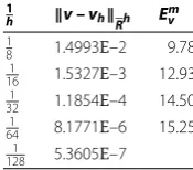
Table 1 Results for the solution
Table 2 First derivative approximation results with the fourth-order accurate formulae
1
Table 3 Second pure derivative approximation results
1
Table 4 First derivative approximation results with the fifth-order accurate formulae
1
LetUbe the exact solution of the continuous problem, andUhbe its approximate values
onRh. We denoteU–UhRh=max
In Tables and , the maximum errors and the order of convergence of the approxi-mate solution for different step sizeshare given, which corresponds to order of accuracy
O(h|lnh|). In Tables and , the results for the first and pure second derivatives of prob-lem (.) are presented, which correspond toO(h). The results presented in Table show that the accuracy is improved by using the fifth-order accurate formulae for the same con-ditions imposed on the given boundary functions.
6 Conclusion
deriva-tives at the rate ofO(h) is proved. It is shown that the accuracy for the approximate value of the first derivatives can be improved up toO(h|lnh|) for the same boundary functions by using the fifth-order formulae on some faces of the parallelepiped.
The obtained results can be used to justify finding the above-mentioned derivatives of the solution of D Laplace boundary value problems on domains described as unions or as intersections of a finite number of rectangular parallelepipeds by the difference method, using the Schwarz or Schwarz-Neumann iterations (see [–]).
Competing interests
The authors declare that they have no competing interests.
Authors’ contributions
All authors contributed equally to the writing of this paper. All authors read and approved the final manuscript.
Author details
1Department of Mathematics, Near East University, Nicosia, KKTC, Mersin 10, Turkey.2Department of Mathematics,
Eastern Mediterranean University, Gazimagosa, KKTC, Mersin 10, Turkey.
Received: 10 February 2016 Accepted: 19 May 2016
References
1. Lebedev, VI: Evaluation of the error involved in the grid method for Newmann’s two dimensional problem. Sov. Math. Dokl.1, 703-705 (1960)
2. Volkov, EA: On convergence inC2of a difference solution of the Laplace equation on a rectangle. Russ. J. Numer. Anal. Math. Model.14(3), 291-298 (1999)
3. Dosiyev, AA, Sadeghi, HM: A fourth order accurate approximation of the first and pure second derivatives of the Laplace equation on a rectangle. Adv. Differ. Equ.2015, 67 (2015). doi:10.1186/s13662-015-0408-8
4. Volkov, EA: On the convergence inC1
hof the difference solution to the Laplace equation in a rectangular
parallelepiped. Comput. Math. Math. Phys.45(9), 1531-1537 (2005)
5. Volkov, EA: On the grid method for approximating the derivatives of the solution of the Dirichlet problem for the Laplace equation on the rectangular parallelepiped. Russ. J. Numer. Anal. Math. Model.19(3), 269-278 (2004) 6. Volkov, EA: On differential properties of solutions of the Laplace and Poisson equations on a parallelepiped and
efficient error estimates of the method of nets. Proc. Steklov Inst. Math.105, 54-78 (1969) 7. Mikhailov, VP: Partial Differential Equations. Mir, Moscow (1978)
8. Mikeladze, SE: On the numerical solution of Laplace’s and Poisson’s differential equations. Izv. Acad. Nauk SSSR, Ser. Mat.2, 271-292 (1938)
9. Samarskii, AA: The Theory of Difference Schemes. Dekker, New York (2001)
10. Volkov, EA, Dosiyev, AA: A highly accurate homogeneous scheme for solving the Laplace equation on a rectangular parallelepiped with boundary values inCk,1. Comput. Math. Math. Phys.52(6), 879-886 (2012)
11. Burder, RL, Douglas Faires, J: Numerical Analysis. Brooks/Cole, Cengage Learning, Boston (2011) 12. Bakhvalov, NS, Zhidkov, NP, Kobelkov, GM: Numerical Methods. Nauka, Moscow (1987) (in Russian) 13. Kantorovich, LV, Krylov, VI: Approximate Methods of Higher Analysis. Noordhoff, Groningen (1958)
14. Badea, L: On the Schwarz-Neumann method with an arbitrary number of domains. IMA J. Numer. Anal.24, 215-238 (2004)
15. Dosiyev, AA: The high accurate block-grid method for solving Laplace’s boundary value problem with singularities. SIAM J. Numer. Anal.42(1), 153-178 (2004)
16. Volkov, EA, Dosiyev, AA: A high accurate composite grid method for solving Laplace’s boundary value problems with singularities. Russ. J. Numer. Anal. Math. Model.22(3), 291-307 (2007)
17. Dosiyev, AA: The block-grid method for the approximation of the pure second order derivatives for the solution of Laplace’s equation on a staircase polygon. J. Comput. Appl. Math.259, 14-23 (2014)
18. Dosiyev, AA, Buranay, CS, Subasi, D: The block-grid method for solving Laplace’s equation on polygons with nonanalytic boundary conditions. Bound. Value Probl.2010, Article ID 468594 (2010). doi:10.1155/2010/468594 19. Dosiyev, AA, Celiker, E: Approximation on the hexagonal grid of the Dirichlet problem for Laplace’s equation. Bound.