ECG Signal Compression using Improvised Error Back Propagation Neural Network with GDAL

(1)

Vol. 5, Issue 3, March 2017

ECG Signal Compression using Improvised

Error Back Propagation Neural Network with

GDAL

Dr.Mridul Kumar Mathur1, Madhukeshwar F. Khanpur2

Asst. Professor (Selection Grade), Dept. of Computer Science, LMCST, Jodhpur (Raj.), India1

Ph.D. Research Scholar, Dept. of Computer Engineering, Jodhpur National University (JNU), Jodhpur (Raj.), India 2

ABSTRACT: Electrocardiogram (ECG) data is bulky in size and needs to compress through suitable compression techniques for reducing storage requirement s and to transfer ECG signal over low bandwidth channel in less time over the network. In this paper we have applied a novel approach of improvised Error Back Propagation Neural Network with Gradient Descent Learning rate for network to learn with in an adaptive manner. In our experiments we have found that an average compression ratio of 9 and Percentage Mean square Error (PRD) between 2 to 7 is achieved with this method. In addition to that the network learns faster than the tradition neural network after implementing Gradient Learning mechanism.

KEYWORDS: Electrocardiogram, Gradient descent learning, Compression Ratio, Percentage Mean Root Square Difference

I. INTRODUCTION

ECG signal depicts the exact picture of the activities associated with the functioning of the heart. After examining an ECG signal various heart diseases can be diagnosed. Furthermore, ECG signal needs to be compressed for reducing its size for rapid transmission and economical storage.

Even though the processor speed, bandwidth and storage capacity has been increased tremendously the demand for ECG compression has been still in picture. The main objective of ECG compression is to reduce redundancy presented in the ECG signal without loss of clinical information and the reconstructed signal must contain all the clinical features intact for diagnosis purpose.

1.1 Types of Compression Techniques:

The compression algorithms can be broadly classified [1, 2] into two categories:

(A) Lossless Compression:

In this type of compression the reconstructedsignal is exact replica of the original signal and there is no loss of information in that reconstructed signal at all. The reconstructed signal is identical to the original signal. This type of compression comes under the category of lossless signal compression.

(B) Lossy Compression:

(2)

1.2PERFORMANCEEVALUATION

The effectiveness of ECG compression techniques is described in terms of Compression Ratio[6] (CR) and Percentage Mean Square Difference (PRD)[6].The quality of reconstructed ECG signal can be examined with these criteria.

1.2.1 Compression Ratio (CR)

It is defined as the ratio of original data to compressed data without considering factors such as bandwidth, sampling rate, word length, reconstruction error, noise level etc. The CR is the ratio of the original file size to the compressed file size, given as follows:

Size

File

Compressed

Size

File

Original



CR

(1.1)

Larger the CR better is the compression.

1.2.2 Percentage Root Mean Square Difference (PRD)

PRD is measurement of percentage error. This factor evaluates the distortion regarding the difference between the original and the reconstructed signal. The factor can be represented by the following formula. The definition of the PRD is given by following equation:

 





100

] [ 1 2 1 2 X n x n x n x PRD _N n N n



           (1.2)

where

x

 

n

and

x

 

n



are the original and reconstructed signals, respectively; and N its length. For better reconstruction of the original signal, the values of the PRD should be very low.Thus collectively we require large CR and smaller PRD for better compression.

1.3 Types of Artificial Neural Networks

Artificial Neural Network topologies are classified intotwo categories [7,8]:

1. Feed Forward ANN

In this type of neural network information flow is unidirectional. This network has no feedback (loops) i.e. the output of one layer has no effect on other layer. Feed-forward ANNs tend to be straight forward networks that associate inputs with outputs .They are used in pattern generation/recognition/classification[7, 8]. They have fixed inputs and outputs.

2. Feed Back ANN

The signals can travel in both the directions in Feedback networks byimplementing loops in the network Feedback networks are dynamic; their 'state' is changing continuously until they reach an saturation point.

1.4 Working of ANNs

Each connection between two nodes has some weight, a real number that carries the information. Their weights are adjusted until the desired output is obtained.

Learning in ANNs

(3)

 Supervised Learning− this is also known as Associative learning. In this matching output pattern is also presented to the network along with the input. Input patterns learn and they are tuned and classified to the matching input patterns.

 Unsupervised Learning− Here the network learns from provided input patterns .It creates a class itself

without external help and tuned accordingly. It learns from its own classes and different types of patterns presented in it.

1.5 Error Back Propagation Neural Network-

The Back propagation [11] was invented by Bryson and Ho in 1969 which is a method for learning in multi-layer network. The Back propagation algorithm is a sensible approach for dividing the contribution of each weight.

There are two differences for the updating rule:

1) The activation of the hidden unit is used instead of activation of the input value. 2) The rule contains a term for the gradient of the activation function.

II. RELATED WORK

2.1 Literature Review of ECG Signal Compression Techniques

ECG signal compression is required for efficient storage and fast transmission of ECG signal over a low bandwidth channel. Several algorithms have been developed for compression of ECG signal in a way such that the clinical contents will remain intact after reconstruction for diagnostic purpose. For above mentioned objective a literature review on previous work on different ECG compression techniques has been carried out for lossless and lossy data compression techniques.

(4)

III. METHODOLOGY

The neural network for Error Back Propagation is designed Gradient Descent with Adaptive Learning Rate Back propagation mechanism with MATLAB Tool box. A proper learning rate must be chosen for proper learning at efficient convergence [19]. In Gradient Descent Adaptive learning rate mechanism first the initial network and error are calculated and at every epoch new weights and biases are calculated using the current learning rate. The network adopts the new learning rates and new outputs and errors are again calculated for adaptive learning[20,21]. This algorithm shows the steps for this procedure.

Algorithm

1. Initialize network with random weights 2. For all training cases (called examples):

a. Present training inputs to network and calculate output b. For all layers (starting with output layer, back to input layer): i. Compare network output with correct output (error function) ii. Adapt weights in current layer

3. Method for learning weights in feed-forward (FF) nets 4. Use gradient descent to minimize the error

 Propagate deltas to adjust for errors backward from outputs to hidden layers to inputs 5. After training the compressed file contains compressed signal.

6. Compressed file is used to reconstured signal.

7. Compression Ratio, Root Mean Square Difference is calculated to identify the quality of reconstructed signal.

Figure 1 shows architecture of the Error Back Propagation Neural Network with hidden layer[22].

Figure 1: Architecture of Error BackPropagation Algorithm with hidden layer

IV. EXPERIMENTAL RESULTS

4.1 Experimental Results

(5)

4.1.1 Performance Evaluation

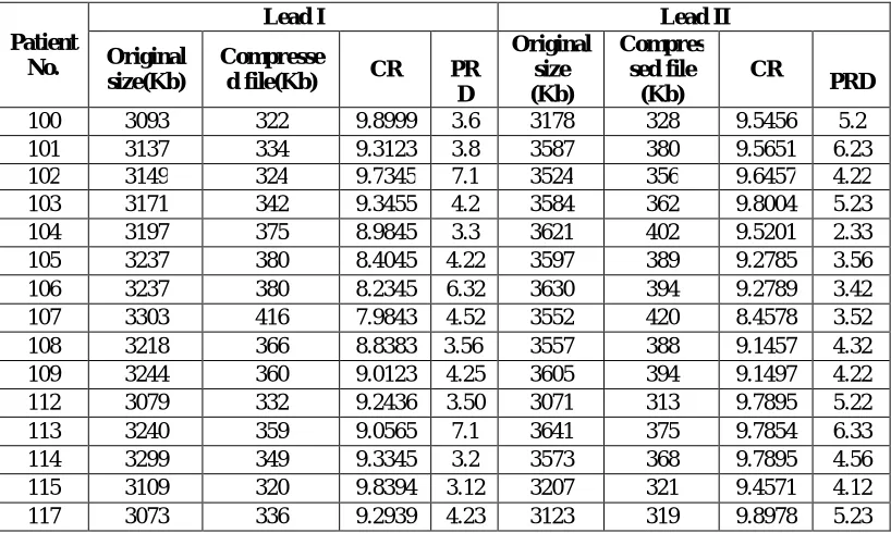
To authenticate the reconstruction of the original data from this algorithm, a performance criterion is needed. For this, we have taken percentage root mean-square difference (PRD) [9] and Compression Ratio (CR) [9] as performance measure which has already been explained in previous section. Both the leads of 15 patients are reconstructed using this method. Table 1 shows the CR and PRD of both leads of 15 patients after reconstruction. This table also shows the original file size along with the size of compressed file.

Table 1: CR and PRD of Lead I and Lead II of 15 Patients

It can be seen from this table highest CR of 9.8999is achieved for Lead I of patient 100. Similarly the lowest CR of 7.9843is obtained for Lead I of patient 107.PRD obtained for both the leads of all the patients varies in the range of 2 to 7 .This implies that very negligible loss of information is there. This method has a limitation that CR up to a certain limit can be achieved with this method. An average CR of 9 is achieved with this method.

4.2 Comparison of Original and Reconstructed ECG signal

The Original and reconstructed signal of the lead I of patient 101 is shown in figure 2.It can be seen in this figure that the original signal is same as reconstructed signal.

Patient No.

Lead I Lead II

Original size(Kb)

Compresse

d file(Kb) CR PR

D

Original size (Kb)

Compres sed file

(Kb)

CR

PRD

(6)

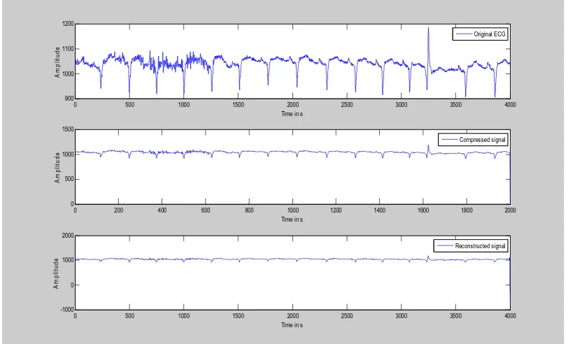
Figure 2:Original and Reconstructed signal of Patient 101 with first 4000 samples (Lead I)

To prove that the reconstructed signal is almost same as originalsignal, these are placed in sub plotted form. The compressed signal is also shown with the original signal and reconstructed signal. It can be seen from this figure the signal is reconstructed properly and with very low loss of information.

(7)

Figure 4: Original and Reconstructed signal of Patient 103 with first 4000 samples (Lead I)

Figure 3 and 4 show the same for the patient 100 and 103 and similar results can be seen for all the patients. Therefore, this method is very useful for compression and retains all the clinical properties of ECG signal after reconstruction.

Figure 5: Original and Reconstructed signal of Patient 101 with first 4000 samples (Lead II)

0 500 1000 1500 2000 2500 3000 3500 4000

600 700 800 900 1000

Time in s

A

m

p

li

tu

d

e

Original ECG

0 200 400 600 800 1000 1200 1400 1600 1800 2000

0 500 1000

Time in s

A

m

p

li

tu

d

e

Compressed signal

0 500 1000 1500 2000 2500 3000 3500 4000

-1000 -500 0 500 1000

Time in s

A

m

p

lit

u

d

e

(8)

Figure 6:Original and Reconstructed signal of Patient 100 with first 4000 samples (Lead II)

Figure 7: Original and Reconstructed signal of Patient 105 with first 4000 samples (Lead II)

Figure 5, 6 and 7 show second lead for the same for the patient 101,100 and 103 and similar results can be seen for all the patients. Both the leads of all the patients have been successfully reconstructed.

0 500 1000 1500 2000 2500 3000 3500 4000

900 1000 1100 1200

Time in s

A m p lit u d e Original ECG

0 200 400 600 800 1000 1200 1400 1600 1800 2000

0 500 1000 1500

Time in s

A m p li tu d e Compressed signal

0 500 1000 1500 2000 2500 3000 3500 4000

-1000 0 1000 2000

Time in s

A m p li tu d e Reconstructed signal

0 500 1000 1500 2000 2500 3000 3500 4000

600 800 1000 1200 1400

Time in s

A m p li tu d e

0 200 400 600 800 1000 1200 1400 1600 1800 2000

0 500 1000 1500

Time in s

A m p li tu d e

0 500 1000 1500 2000 2500 3000 3500 4000

-1000 0 1000 2000

Time in s

(9)

V. CONCLUSION

This method has been applied on both the leads of 15 subjects from MIT-BIH Arrthymia database.An improvised BackPropagation algorithm has been used with Gradient Descent Adaptive learning mechanism in which the learning rate is adaptive in nature and it is changed dynamically for better convergence and learning. Original signal is compressed and reconstructed and afterwards, CR and PRD of both the leads of the 15 subjects iscalculated. A good compression ratio of average 9 is achieved with a very low error with a good recons trued signal quality.

REFRENECES

[1]Bell, Timothy C., Cleary, John G., Witten, Ian H,(1990) Text Compression, Prentice Hall, Englewood Cliffs NJ. [2] David Salomon, Data Compression - The Complete Reference, Springer, 3rd edition (2004).

[3]Cetin, A. E., Köymen, H. “Compression of Digital Biomedical Signals.” The Biomedical Engineering Handbook: Second Edition. [4] Karl, John H., An Introduction to Digital Signal Processing, Academic Press, 1989.

[5]Khalid Sayood, Introduction to data compression, Morgan Kaufmann, 3rd edition (2005).

[6] M. Blanco-Velasco, F. Cruz-Roldán, J. I. Godino-Llorente, J. Blanco-Velasco, C. Armiens-Aparicio, and F. López-Ferreras, On the Use of PRD and CR Parameters for ECG Compression, International Journal on Medical Engineering & Physics 27(6) (2005) 798-802,http://dx.doi.org/10.1016/j.medengphy.2005.02.007.

[7] Martin T. Hagan, Howard B. Demuth, Mark Beale, “Neural Network Design”, China Machine Press, 2002. [8] M. Hajek, “Neural Networks”, 2005.

[9] R. Rojas, “Neural Networks”, Springer-Verlag, Berlin, 1996,

[10]Simon Haykin, “Neural Networks-A comprehensive Foundation”, IInd Edition,Pearson Education (Singapore), 2004, pp 465- 500.

[11]D. Nguyen and B. Widrow, Improving the learning speed of 2-layer neural network bychoosing initial values of the adaptive weights, IEEE First International Joint Conferenceon Neural Networks, 3, 21–26, (1990).

[12]G. Liliana, M. Fernando, and P. Gianfranco, “ECG data compression through adaptive sampling and arithmetic coding,” Annual International conference of the IEEE Engineering in Medical and Biology Society, Vol. 12, No. 1, pp. 451–452,1990.

[13] Ali Bilgin and W. Marcellin, “Compression of electrocardiogram signals using JPEG2000 “IEEE Transaction on Consumer Electronics, Vol.49, No.4, Nov. 2003.

[14]C. M. Fira, L. Goras, and S. Member, “An ECG Signals Compression Method and Its Validation Using NNs,” IEEE Transactions on Biomedical Engineering Vol . 55, No. 4, pp. 1319–1326, 2008.

[15]T.P. Abenstein, “Algorithms for real time ambulatory ECG monitoring, “Biomedical Science Instrumentation Vol 12, pp 73-79, 1978.

[16]T.R. Cox, F.M. Noble, “AZTEC, A Preprocessing Program for Real-Time ECG Rhythm Analysis, “, IEEE Trans. on BME, April 1968.

[17]E. Betri et al, “ECG data compression using double logarithmic quantisation of Walsh spectrum,” IEE Electronics letters, vol. 31, pp. 1025-1026, 1995.

[18]S. Olmos, M. Millan, J. Garcia, and P. Laguna,” ECG data compression with the Karhunen–Loèvetransform.,” Computer in Cardiology pp 253–256,1990.

[19]E. Polak, Optimization: Algorithms and Consistent Approximations, Springer-Verlag,(1997).

[20]D.E. Rumelhart and J.L. McClelland(eds), Parallel distributed processing: explorationsin the microstructure of cognition, Vol. 1: Foundations, MIT Press, (1986).

[21] T.P. Vogl, J.K. Mangis, J.K. Rigler, W.T. Zink and D.L. Alkon, Accelerating theconvergence of the back-propagation method, Biological Cybernetics, 59, 257–263,(1988).