An Algorithmic Study of Link Prediction in
Social Network Sites
Suryakumar B, Dr.E.Ramadevi
Ph.D Research Scholar, Department of Computer Science, NGM College, Pollachi, India Associate Professor, Department of Computer Science, NGM College, Pollachi, India
ABSTRACT: In the area of social network web mining there can be different kinds of links or edges between the nodes are using. The example of them are social contacts, phone calls, hyper-reference etc. Actually the link prediction is the problem of predicting the edges and links that either don’t yet exist at the given period of time t or exist, but have not been discovered are likely in near future. In our work we introduced approaches to link prediction based on various measures for proximity based approaches. For example we can consider a co-authorship network among scientists, e.g. two scientists who are close to the network will have colleagues in common, so they most likely collaborate near future. Out aim is to make betterment in creative notion precise and understandable which measures the most accurate outputs. There are three types of link prediction algorithms are used in social network link prediction. There are path based, node base and meta approaches. The node neighbour approach is based on network local features only. It is mainly focussing nodes structure only. In the case of local based measures Jaccards Coefficient, Adar/Adamic etc. The next type is path based algorithms like Sim-Rank,Katz , the rooted page rank etc. The meta approaches changes the data being passed to one the path based algorithms. The algorithms are clustering algorithms, LR-approximation algorithm, unseenbig rams etc.
KEYWORDS: Social Network, Link Prediction, Social Analysis, Similarity Metric, Learning Model.
I. INTRODUCTION
A Social Structure consists of nodes(Individuals or Organizations) and nodes are connected bydifferent types of relationships. A set of social actors or nodes(such as individuals or organizations) and a set of the dyadic ties between these nodes constitute a social network. For example scientists in a discipline, employees in a large company, business leaders can be thought as nodes in a network and co-authors of a paper, working on a project, serve together on board can be thought as edges respectively. The idea behind Social Networks is to create opportunities to develop friendships, share information and promote business in a network. OSN like Facebook and Twitter have become important part of daily life of millions of people. The enormous growth and dynamics of these networks has led to several researches that examine the network properties i.e. structural and behavioural properties of large scale social networks. Social network is a term used to describe web-based services that allow individuals to create a public/semi-public profile within a domain such that they can communicatively connect with other users within the network [8]. Before the advent of social network, the homepages was popularly used in the late 1990s which made it possible for average internet users to share information[11].
II. LINKPREDICTIONPROBLEM
a paper together will do so in the next few years. Or, when one of the researchers changes institutions, they may come geographically very close. Such interactions are be hard to predict. But by studying the network characteristics, we can predict the possible links that are going to form. Our objective is to make this intuitive notion very exact, and to understand which measures of proximity in a graph lead to accurate predictions.Data mining provides a wide range of techniques for detecting useful knowledge from massive datasets like trends, patterns and rules [9].The link prediction problem is also deals with the problem of getting missing links from a known network, in a number of fields. It involves
prediction of additional links that are not directly visible currently, are likely to exist in a network based on observable data. It considers a static picture of the network, rather than taking network evolution and network dynamics. It also considers specific properties of the nodes in the network, rather than computing the power of prediction methods that
focuses on the graph structureGiven a social network G(V;E) in which an edge represents some kind of interactions between its vertices on nodes at a given time t. Suppose we have a snapshot of a social network at a given time. We choose four times t0 < t00 <t1 < t01, and give our algorithm to predict links that are likely to be formed in the near future from the network G[t0; t00]. That results in predicting new links, not present in G[t0; t00], that are expected to appear in the network G[t1; t01]. Werefer to [t0; t00] as the training interval and [t1; t01] as the test interval [1]. The most basic approach for similarity between any pair of nodes is by taking the length of their shortest path in graph. We rank pairs of nodes in descending order of score(x; y), where score(x; y) is the negative of the shortest path length between x and y. We take a snapshot of a social network as training set and predict the interactions among the nodes of training set that are likely to occur in near future. The algorithms are classified as belows [2].
III.PROPOSEDALGORITHM
The link prediction algorithms based on user input as maximum path to be traversed predicts the probability of formation of link between any two nodes of the network by traversing all the paths of the network up to that certain input path length. It first traverses the path lengths of 2 i.e. the immediate neighbourhoods of the node. we can say it runs a neighbourhood algorithm on path length 2. It then produces a similarity list between every two nodes. When it traverses the graph for path length 3, it uses new paths that are made by path length 2 to get the new the length of the path of three and computes their similarity matrix and updates the similarity matrix in a cumulative way. This process continues till the graph is traversed up to the maximum path length to be traversed given by user. Let we get a path from A to B while traversing for the path length of n−1 with some similarity value, when we traverse the graph for path
length value n, then we will check all the neighbours of B(i.e. C) to get path from A to C. We compute the similarity of each pair (A,C) and update the path list if their no direct link between A and C in the original graph. The inputs to the algorithm are the graph in terms of a list or adjacency array, the total number of nodes the graph, maximum length to be traversed, which determines how many time the algorithm will run and the path length for each specific traversal. The
output of the algorithm is a similarity list containing the similarity value between every two nodes by traversing the path lengths of given maximum user input value. By observing the similarity matrix we can predict the future links. The high similar values have more probability to form links in near future and we can classify the values based on certain threshold value. The similarity values more than the threshold value are likely to form future links. This prediction can be compared with the test data to get the efficiency of the algorithm.
IV.DIFFERENTTYPESOFAGORITHMSINLINKPREDICTION A. Node NeighborhoodAlgorithm
Node neighbourhood meaning the nodes directly connected to the two given nodes. It is simple technique which traverse only paths of length 2. For any node A it check the neighbour of A and computes their similarity with A. It considers only local features of a network, focusing mainly on the nodes structure(i.e. based on the number of common friends that two users share.
B. Common Neighbors
Γ(x)∗Γ(y). This measurement is based on the idea that two nodes a and b have an increased probability to connect if
they have a shared neighbor c. With a growing number of shared neighbours this probability grows even higher. The weighted Common Neighbors(CNw) is defined as follows where w(x,y) is the number of interactions between the
nodes x and y. CNw(x,y) := X z(x)∩Γ(y) w(x,z) + w(y,z) 2
C.Jaccardcoefficient
Jaccardscoeficient measures number of the features(neighbors) that are shared between two nodes commensurate to all features that either one of the nodes has. Jaccardscoefficient[11] is a normalized variation of Common Neighbors [? ]R7). The Jacardcoificient is defined as follows
J(x,y) :=Γ(x)∩Γ(y) Γ(x)∪Γ(y)
This is the Common Neighbors measurement normalized by the union of the node neighborhoods.
D.Adamic/Adar
It is a measurement that compares how many attributes two nodes have in common. They rate items that are unique to a few users more heavily than items shared amongst a huge group of users. This measurement can easily be adjusted in the context of node neighborhood by looking at shared neighbors as an attribute. Therefore the sum over the shared neighbors inverse of the logarithms of their neighborhoods is proposed [3]. The Adamic/Adar is defined as follows AA(x,y) := X zΓ(x)∩Γ(y) 1 log|Γ(z)|
The weighted Adamic/Adar (AAw) is defined as follows where w(x; y) is the number of interactions between the nodes
x and y [4].
AAw(x,y) := X z(x)∩Γ(y) w(x,z) + w(y,z) 2
.1 logPz0εΓ(z) w(z0,z) E. Preferential Attachment
Preferential Attachment is based on the hypothesis that a node x will get new neighbors faster than a node y given y has less neighbors than x. So the probability that a node will form a new link varies with number of its present neighbors. The likelihood of two nodes being connected by an edge based on preferential attachment is measured by multiplying the number of their neighbors [5]. The Preferential Attachment is defined as follows
PA(x,y) := Γ(x).Γ(y)
The weighted Preferential Attachment (PAw) is defined as follows where w(x,y) is the number of interactions between the nodes x and y: PAw(x,y) := X x,Γ(x) w(x,x0).Γy0εΓ(y)w(y0,y)
V. PATHBASEDALGORITHMS
Some measurements of link prediction take all paths between two nodes in consideration. The computation of graphs that take the entire graph in consideration is by nature much more complex than node neighborhood algorithms.
A. Katz
A measurement that takes all paths between two nodes in consideration while rating short paths more heavily. The measurement exponentially reduce the contribution of a path to the measure in order to give less weightage longer
paths. Therefore it uses a factor of βl where l is the path length. The Katz is defined as follows
K(x,y) :=∞ X l=1
βl.|paths<l>x,y |
where paths<l>x,y the set of all paths from source x to destination y that have the path length l.
B.Unweighted : paths<l>x,y = 1, if x and y have collaborated and 0 otherwise • Weighted : paths<l>x,y is the number of times that x and y have collaborated
The β can be used to control how much the length of the paths should be considered. A very small β concludes to an
C.SimRank
If two nodes are referenced by more similar objects, then the two nodes have large similarity value. Every object obviously has a similarity score of 1 to itself. Node x and node y are then similar to the degree they are joined to similar neighbours [7]. The SimRank is defined as follows[12]
S(x,x) := 1 S(x,y) := γ.PaΓ(x)PbΓ(y) S(x,y) Γ(x).Γ(y)
γ is a constant with γ[0,1]. The constant can be thought of as a confidence level. If you consider a situation in which
a and b are both neighbours to c, thanobviously the similarity of c to itself is 1, but we do not want to conclude that s(a,b) = s(c,c) = 1. Instead we let s(a,b) = γ ∗ s(x,x) because we are not as confident about the similarity of a and b as
we are about s(x,x) = 1.
D. Hitting Time and Commute Time
Starting from a node x a random walk on a given graph moves iteratively over the graph while choosing the next node each step at random. The expected number of steps to get from x to y via a random walk is defined as the Hitting Time
H(x,y). A short hitting time implies node similarity and therefor a heightened chance of future linking. The commute time C(x,y) is a variant of Hitting time which is useful for undirected graphs, because the hitting time is not symmetric. Therefore it is defined as follows:
C(x,y) := H(x,y) + H(y,x)
The commute time can have high variance, hence, prediction by this feature can be poor. If z is a node with high stationary probability far o x and y, then a random walker would probably reach the ff neighbourhood of z. To avoid that we can use reset the random walker to x with a fixed probability of α.
two normalized versions Hitting Time normalized (Hn) and Commute-Time normalized (Cn) are defined where πx is the stationary probability of x to safeguard it against vertices with a very high π:
Hn(x,y) := −H(x,y).πy Cn(x,y) := −(H(x,y).πy + H(y,x).πx)
VI.THEPROPOSEDALGORITHM
The link prediction algorithms based on user input as maximum path to be traversed predicts the probability of formation of link between any two nodes of the network by traversing all the paths of the network up to that certain input path length. It first traverses the path lengths of 2 i.e. the immediate neighbourhoods of the node. we can say it runs a neighbourhood algorithm on path length 2. It then produces a similarity list between every two nodes. When it traverses the graph for path length 3, it uses new paths that are made by path length 2 to get the new path lengths of 3 and computes their similarity matrix and updates the similarity matrix in a cumulative way. This process continues till the graph is traversed up to the maximum path length to be traversed given by user. Let we get a path from A to B while traversing for the path length of n-1 with some similarity value, when we traverse the graph for path length value n, then we will check all the neighbors of B(i.e. C) to get path from A to C. We compute the similarity of each pair (A;C) and update the path list if their no direct link between A and C in the original graph.
The inputs to the algorithm are the graph in terms of a list or adjacency array, the total number of nodes the graph, maximum length to be traversed, whichdetermines how many time the algorithm will run and the path length for each specific traversal. The output of the algorithm is a similarity list containing the similarity value between every two nodes by traversing the path lengths of given maximum user input value. By observing the similarity matrix we can predict the future links. The high similar values have more probability to form links in near future and we can classify the values based on certain threshold value. The similarity values more than the threshold value are likely to form future links. This prediction can be compared with the test data to get the efficiency of the algorithm.
For each path length, we have to follow many steps:
• Calculate that path list with respect to the list with previous input path value • Update the current adjacency list for the entries having nonzero path value • Calculate the similarity measure with respect to the corresponding path list • Update the similarity list by adding the new similarity measures to the list • Increment the path length
a) Input Parameters
• A : adjacency matrix of undirected and unweighted graph • n : total number of nodes of the graph
• l : max length of path to be explored in G • m : the length of a path for current iteration b)Output Parameters
• sim(i,j) : Similarity measure between nodes i and j
VII.ALGORITHM
Algorithm 1: MAIN FUNCTION for m ← 2 to n do
cpath(A,n,prev,or) sim←simi(sim,path,n,m); path ← 0 ;
end
The main Program iteratively calls for checking the new collaboration between any two nodes for a specific path length
through cpath function and computes thesimilarity between the new collaborations with exactly m path length and updates the similarity measures through sim function.
Fori← 1 to N do for j ← 1 to N do if i< j then if or (i,j) 6= j then for k ← 1 to N do if prev (i,k) 6= 0 then
if A (i,k) 6= 0 and or (k,j) 6= 0 then path (i,j) ← path (i,j)+prev (i,k) * or (k,j) ; end
end end
path (j,i) ← path (i,j) ; end
end end end
prev← path; for i← 1 to N do for j ← 1 to N do if path (i,j) 6= 0 then A (j,i) ← 1 ;
End End End
return path and A;
The cpath function first checks whether there is path from any two nodes of m path length. It checks it by merging the
new paths generated while traversing the previous path length (m−1) and their neighbours in the original graph. So pathmatrix contains new collaborations of path length exactly m.
for i← 1 to n do for j ← 1 to n do lower ← 1; for k ← 1 to m do lower ← lower * (n-k) ; end
sim (i,j) ← ( 1/(m-1)* sim (i,j) ) / lower; end end return sim;
The simi function _nds the similarity measure for every pair of nodes which have path length exactly m. It then cumulates the similarity values till the path length of l for every two nodes. The pair of nodes having higher value of similarity are more likely to form link in the near future.
VIII. OUR PROPOSED METHOD IMPIMENTATION
TABLE I
Figure 3. Comparison Table
Figure4: Link Prediction Analysis
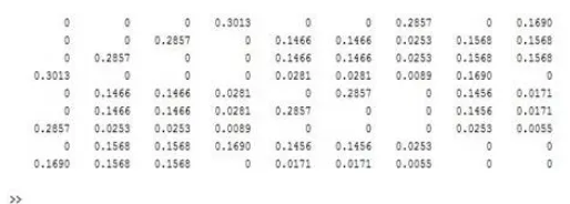
The algorithm is implemented using maximum length to be traversed as 4. This result shows that the similarity value of the node pair U1 and U4 is maximum
Figure 2: Similarity matrix
IX. CONCLUSION
Link Prediction is the method to predict the possible future interactions among the nodes in the near future. Our algorithm uses both global and local characteristics of the network to predict the links. Global approaches has the time constraint as they traverse all paths of network to predict the links and local approaches are less efficient as they consider only local features of the node. Our approach is compared with all the approaches and it provides efficient and accurate friend suggestions in a less interval of time.
X.FUTURE RESEARCH OPERTUNITIES
Link Prediction based on other features like photo, video tagging can be used for better prediction. As many features as we consider simultaneously, the prediction will be better because it gives information about many ways peoples may by connected. We can consider the positive as well as negative links in a network. If positive weight is for support, then negative weight should be for opposing it. As network is always dynamic, so we can consider network dynamics into consideration.
REFERENCES
1] David Liben-Nowell and Jon Kleinberg. The link-prediction problem for so-cial networks. Journal of the American society for information science andtechnology, 58(7):1019{1031, 2007.
[2] Ryan N Lichtenwalter, Jake T Lussier, and Nitesh V Chawla. New per-spectives and methods in link prediction. In Proceedings of the 16th ACMSIGKDD international conference on Knowledge discovery and data mining, pages 243{252. ACM, 2010.
[3] Lada A Adamic and Eytan Adar. Friends and neighbors on the web. Social networks, 25(3):211{230, 2003.
[4] Tsuyoshi Murata and SakikoMoriyasu. Link prediction based on structural properties of online social networks. New Generation Computing, 26(3):245{257, 2008.
[5] A Papadimitriou, P Symeonidis, and Y Manolopoulos. Friendlink: Link pre-diction in social networks via bounded local path traversal. In Computa-tional Aspects of Social Networks (CASoN), 2011 International Conferenceon, pages 66{71. IEEE, 2011.
[6] Han Hee Song, Tae Won Cho, Vacha Dave, Yin Zhang, and LiliQiu. Scal-able proximity estimation and link prediction in online social networks. InProceedings of the 9th ACM SIGCOMM conference on Internet measurement
conference, pages 322{335. ACM, 2009.
[7] Glen Jeh and Jennifer Widom. Simrank: a measure of structural-context similarity. In Proceedings of the eighth ACM SIGKDD international conference on Knowledge discovery and data mining, pages 538{543. ACM, 2002.
[8] Chen, Z. S., Kalashnikov, D. V. and Mehrotra, S. Exploiting context analysis for combining multiple entity resolution systems. In Proceedings of the 2009 ACM International Conference on Management of Data (SIGMOD'09), 2009. [9]. Kagdi, H., Collard, M. L., Maletic, J. I.: A survey and taxonomy of approaches for mining software repositories in the context of software evolution. J. Softw. Maint. Evol.: Res. Pract, 19, 77-131, 2007.
[10]. Becker, H., Iter, D., Naaman, M., Gravano, L.: Identifying content for planned events across social media sites. In Proceedings of the fifth ACM international conference on Web search and data mining (pp. 533-542). ACM, 2012.
[11].M. A. Hasan, V. Chaoji, S. Salem, and M. Zaki, “Link prediction using supervised learning,” in SDM Workshop of Link Analysis, San Francisco, Calif, USA, 2006.
[12]. G. Jeh, J. Widom, SimRank: a measure of structural-context similarity, in: Proceedings of the ACM SIGKDD International Conference on Knowledge Discovery and Data Mining, ACM Press, New York, 2002, pp. 271–279.
BIOGRAPHY
B.Suryakumar received M.Sc and MCA degrees in Computer Science from Annamalai University, Tamilnadu. Currently he is doing PhD in Computer Science at Bharathiar University, Coimbatore. His research interest lies in the area of Data Mining ,Networking and Data security.