Sparse Regularization for Inverse Problems Governed by Evolution Equations.

(1)

ABSTRACT

HUMBER, CARY ROSS. Sparse Regularization for Inverse Problems Governed by Evolution Equations. (Under the direction of Kazufumi Ito.)

The purpose of this thesis is twofold. Firstly, we introduce a novel method for es-timating the state of a system governed by a linear evolution equation. The method utilizes the adjoint of the partial differential equation (PDE) and a basis for the Hilbert space to accurately reconstruct the initial condition. The method also provides a filter bank which can be utilized for the purpose of reconstructing initial conditions based on given data. We then extend the method to include source identification and simultaneous state/parameter estimation for a certain class of problems.

(2)

c

(3)

Sparse Regularization for Inverse Problems Governed by Evolution Equations

by

Cary Ross Humber

A dissertation submitted to the Graduate Faculty of North Carolina State University

in partial fulfillment of the requirements for the Degree of

Doctor of Philosophy

Applied Mathematics

Raleigh, North Carolina 2011

APPROVED BY:

Alina Chertock Pierre Gremaud

Zhilin Li Ralph Smith

Kazufumi Ito

(4)

DEDICATION

(5)

BIOGRAPHY

(6)

ACKNOWLEDGEMENTS

I would like to express my gratitude to my advisor, Professor Kazufumi Ito, for his guidance and insight while working with him. His encouragement and interest in my work proved to be invaluable.

I am also appreciative for the members of my committee, including Professor Ralph Smith for serving as a last minute substitute.

I would like to express my appreciation for the In-House Laboratory Independent Research (ILIR) program at the Naval Surface Warfare Center, Panama City, Fl, for hosting me during the last research period of my Ph.D. program.

I would also like to express my gratitude to Dr. Quyen Huynh of NSWC-PC for his support and encouragement during the final stages of my Ph.D.

(7)

LIST OF FIGURES

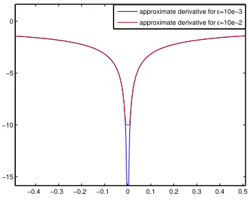
Figure 5.0.1 Comparison of approximate subdifferentials for ε = 10e−3 _and

ε = 10e−2_. _{. . . .} ₆₄

Figure 6.1.1 Measurements taken for 1-D diffusion equation . . . 72

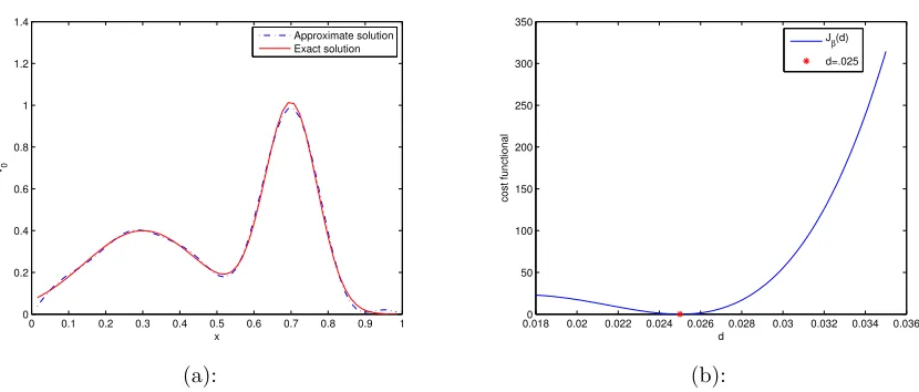
Figure 6.1.2 1-D reconstruction for diffusion equation . . . 73

Figure 6.1.3 Control corresponding to sin(2πx). . . 74

Figure 6.1.4 1-D reconstruction for variable coefficient diffusion equation . . . 75

Figure 6.1.5 1-D reconstruction for variable coefficient diffusion equation . . . 75

Figure 6.1.6 Comparison using different basis functions . . . 76

Figure 6.1.7 Simultaneous state/parameter estimation for 1-D diffusion equation 77 Figure 6.1.8 Results for simultaneous state/parameter estimation of 1-D diffu-sion equation . . . 77

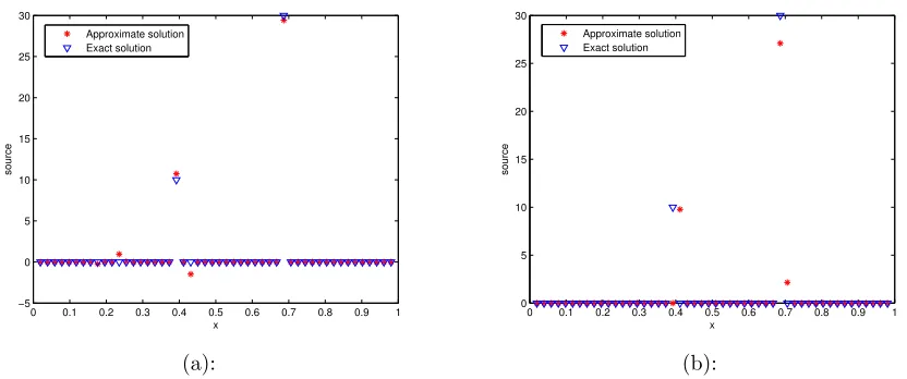
Figure 6.1.9 Point source identification for 1-D diffusion equation . . . 79

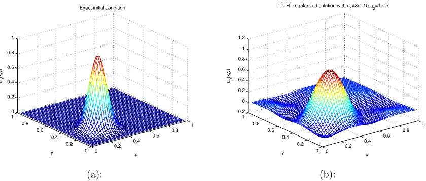
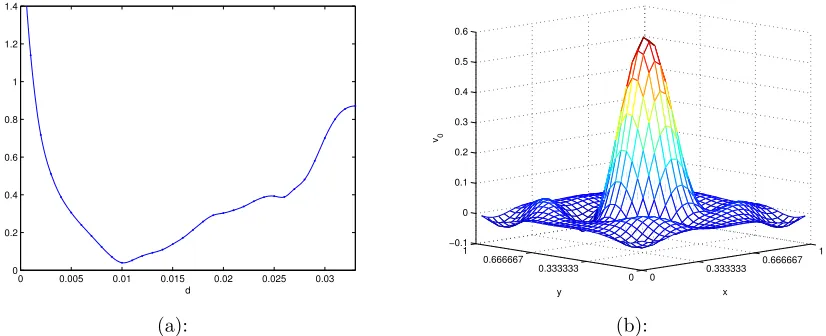
Figure 6.2.1 2-D reconstruction for diffusion equation . . . 81

Figure 6.2.2 Results for simultaneous state/parameter estimation of 2-D diffu-sion equation . . . 82

Figure 6.2.3 Measurements taken for 2-D point source identification . . . 83

Figure 6.2.4 2-D point source identification for 2-D diffusion equation . . . 84

Figure 6.3.1 Measurements and locations for 2-D convection-diffusion equation 86 Figure 6.3.2 Reconstruction for 2-D convection-diffusion equation . . . 86

Figure 6.3.3 Comparison of 2-D convection-diffusion and diffusion equations . 87 Figure 6.3.4 2-D state/parameter estimation for convection diffusion . . . 88

Figure 7.1.1 Cues for the wrist up action. . . 91

Figure 7.1.2 Comparison of weights for different `p norms. . . 91

Figure 7.1.3 Comparison of PSVM and nonsmooth formulation. . . 92

Figure 7.1.4 Comparison of data classifiers . . . 92

Figure 7.2.1 Synthetic Aperture Sonar setup. . . 93

(10)

Chapter 1 Introduction

1.1 Motivation

The motivation for this thesis originates from the practical needs of many classically difficult inverse problems in the mathematical sciences, as well as some of the more re-cent needs throughout the sciences. The primary mathematical focus of this thesis is the solution of inverse problems for the purpose of reconstructing states and identifying parameters of evolution equations. Roughly speaking, inverse problems involve deter-mining a solution to a problem for which the governing dynamics are known, and the measurements, or output, of the system are given. For instance, one may be given a time series, or sampling, of the current heat profile of a metal plate and be asked what the initial heat profile was one hour prior. Of course, if a full history of data is available its just a matter of searching in the right place. Many of the most interesting and relevant scientific problems involve an incomplete time history of data. This is the case either be-cause of storage constraints or due to unavailability/inaccessibility of data. In addition, the data may be sparsely distributed across the “area” being measured.

(11)

domain in time, or the measurements are only available for select time values, such as the final time. Not only is it necessary to reconstruct solutions from sparse measurements for obvious reasons, but the ability to reconstruct solutions from a sparse set of data can help mitigate the constant flood of data. This thesis seeks to generalize some of the work already produced in the field of dynamical inverse problems and to improve upon the solution methods for stable reconstruction.

Not only is there increased interest in data reduction/sparsity, but there is increased motivation for robust algorithms that can adapt to varying noise levels in the data. Problems such as numerical weather prediction involve solving large scientific problems repeatedly throughout the day (and night). It is desired for the algorithms to adapt to changes in the data and to fluctuations in noise levels. We utilize the Tikhonov type regularization to stably construct solutions, where the parameters are chosen based on a priori information. Given the needs of the scientific community, the two concepts of sparsity/compression and adaptability/tunability are at the forefront throughout this thesis.

As a consequence of the methods developed in this thesis, we are able to effectively deal with some of the problems involved with large datasets, effectively mining the data. Though the availability of data can certainly be a blessing, there are difficulties that must be overcome when dealing with large datasets. The ever-growing size and availability of data plagues many already difficult problems. Not only that, but it has become increasingly apparent over the last several years that some problems can be solved given very little data in comparison to the size of the problem (i.e., compressed sensing [7]). This is good news for mathematicians tasked with solving difficult problems, but it also provides opportunity for developing hardware and software capable of efficiently utilizing compressed data. Of course, this thesis is void of hardware/software issues, however many questions remain pertaining to compressed sensing, sparsity optimization and general inverse problem theory for systems governed by evolution equations.

In the general framework, we consider the inverse (deconvolution) problem of the form

Kv=yδ (1.1.1)

where K is a compact operator. The data, yδ_{, is assumed to be noisy and possibly}

(12)

and continue to be studied, while new applications continue to emerge which fall into this framework. An incomplete list includes computerized tomography, inverse scattering, data assimilation for weather forecasting, and so on. A more complete set of examples can be found in the monographs [9, 11, 22].

As already mentioned, we are particularly motivated by state and parameter esti-mation problems involving systems governed by partial differential equations (PDE). For instance, in the meteorological sciences, one may wish to determine the atmospheric pres-sure or velocity from sensor data. The essential features can be modeled by the (linear) convection-diffusion equation

∂v

∂t =c(x)· ∇v +∇ ·(d(x)∇v) +f(x). (1.1.2)

For this particular problem, the unknown is the state,v(x, t1), at some time in the recent past, t1. In general, the coefficients c, d may be unknown as well. Actual observations are taken at various sample locations. Using the data and the PDE formulation, an approximate past state is solved for, which is then used as the initial condition for a simplified numerical weather prediction. The full formulation of this problem, based on the Navier-Stokes equations, can be found in the paper [14].

Other related, but simpler, PDE that have similar inverse problem formulations are the diffusion equation

∂v

∂t =∇ ·(d(x)∇v) +f(x), (1.1.3)

and the reaction-diffusion equation

∂v

∂t =D∆v+f(v). (1.1.4)

For the corresponding inverse problems, we are given either a time series of sampled solution values, v(x, t), or a sample of the final time solution v(x, tf). That is, certain

(13)

1. For all admissible data, a solution exists, 2. For all admissible data, the solution is unique, 3. The solution depends continuously on the data.

The concept of ill-posedness and methods for dealing with it will be made more clear in Chapter 4. An example of a highly ill-posed problem is the homogeneous backwards heat equation

∂v

∂t =∇ ·(c(x)∇v), x∈Ω (1.1.5)

v(x, tf) = φ(x) (1.1.6)

vΓ = 0, Γ =∂Ω (1.1.7)

due to the amplification of errors by the generalized Fourier expansion of the solution (see [11] for further details). Here, we are solving the heat equation backwards in time, given the final time heat profile. The problem’s difficulty is compounded when the final temperature profile is only available on a subdomain. That is, we are given measurements

y=v(x, tf) x∈Ωs

for some set Ωs ⊂ Ω. For our purposes, we assume the points x ∈ Ωs are sparsely

distributed in Ω. Solving the heat equation backwards introduces large errors due to integrating small errors from the noisy data. Due to the nature of the fundamental solution of the heat equation, the small errors in the data become exponentially amplified. Identifying the initial heat profile from the full final time heat profile is a more classical inverse problem. Modern day problems of this type have evolved to include more practical concerns. For example, as already mentioned, the data may be a partial time series of the solution. In this case, at each time step, the solution may be available for output at select points in the domain, or the data may be available as averages over one or more subdomain. In the latter case, we are given measurements

(14)

where

Cv(t) = 1

µ(Ωs)

Z

Ωs

v(s)dµ

for some set Ωs ⊂Ω having volumeµ(Ωs). If the output available is relatively small, this

is essentially the idea of sparsity/compression, which has become increasingly important over the last several years in the sciences. For instance, the available data may be sparse in comparison to the size of the problem (i.e., 10% of a region may be available for measurement). Given very little information, it is then necessary to reconstruct the solution as accurately as possible. Fortunately, the general theory allows us to do so (see [7]). The need to reconstruct solutions from sparsely available data is not only true for PDE inverse problems, but for the general inverse problem (1.1.1).

In the same way, one may also be interested in reconstructing solutions that are sparsely distributed themselves, rather than the data being sparsely distributed. For example, the initial condition of the heat equation may be a collection of point sources,

δ(x −xj), located at xj. Here, one needs to use the a priori information about the

solution (i.e., sparsity) to assist in the recovery. Other formulations include identifying the unknown coefficients c, d in addition to the initial condition, v(0), being unknown.

To develop and analyze methods for solving problems of the general form (1.1.3), (1.1.2) we cast the PDE as an abstract Cauchy problem of the form

dv

dt(t) = Av(t) (1.1.8)

y(t) = Cv(t) (1.1.9)

where A is the generator of a C0-semigroup, and C is an observation operator. This formulation, and methods for solving inverse problems derived from this formulation, will be discussed in Chapter 2.

1.2 Examples

(15)

PDE that will fall into the general framework. Note that not all of the examples are ac-tually considered in numerical results of this thesis, however, the methods are applicable to each PDE.

Convection-Diffusion Equation

The homogeneous convection-diffusion equation with homogeneous Dirichlet boundary condition is given by

∂v

∂t(x, t) = c(x)· ∇v(x, t) +∇ ·(d(x)∇v(x, t)) (1.2.1)

v(x,0) = v0(x) (1.2.2)

v(x, t) = 0 x∈∂Ω (1.2.3)

where the first term on the right-hand side corresponds to convection, while the second term corresponds to diffusion. The coefficients c, d are the convection and diffusion co-efficients, respectively. The convection-diffusion equation can be thought of as modeling a simplified weather system or of a mass-transport system. In the case of a simplified weather system, our method allows the reconstruction of a past weather state. This is a linear PDE, unlike the Navier-Stokes, so it falls into the framework presented in this thesis without modification.

Wave Equation

The second order linear hyperbolic PDE

∂2v

∂t2(x, t) = c 2

∆v(x, t) (1.2.4)

∂

∂tv(x,0) = ψ(x) (1.2.5)

v(x,0) = 0 (1.2.6)

(16)

Black-Scholes

The Black-Scholes model for pricing European options is described by a parabolic equa-tion of the form

−d

dtv(t, S)−

σ2 2 S

2_v

SS + (r−δ)SvS−rv

= 0 (1.2.7)

v(tf, S) =ψ(S). (1.2.8)

Here, S > 0 denotes the price of the stock, v the value of the share, r >0 is the interest rate, δ the influence of dividends, and σ > 0 is the volatility. Further,T is the maturity date andψis the reward function. Typically, the reward function isψ(S) = max(0, K−S) for the put option and ψ(S) = max(0, S−K) for the call option, where K is the strike price. Interesting inverse problems to consider would be to determine the reward function given the stock index, or to recover the unknown strike priceK. The formulation of such problems is discussed in the paper [21].

Navier-Stokes

It is beyond the scope of this thesis, due to nonlinearity, however the long-term goal includes the extension to the nonlinear case. In this case, inverse problems involving the incompressible Navier-Stokes equations may be considered:

∂ ∂tvi+

n

X

j=1

vj

∂vi

∂xj

= ν∆vi−

∂p ∂xi

+fi(x, t) (x∈Rn, t≥0), (1.2.9)

divv =

n

X

i=1

∂vi

∂xi

= 0 (x∈_Rn_{, t}_≥₀₎_, _(1.2.10)

with initial conditions

v(x,0) = v0(x) (x∈Rn).

In this case, the unknowns may be the initial condition v(x,0), the viscosity ν, or the forcefi.

(17)

solved. It is the goal of this thesis to give new insight into the solution of inverse problems from sparsely distributed data or when the solution itself is assumed to be sparsely distributed. Several applications will be considered in the Numerical Tests section of this thesis which demonstrate the applicability of the methods developed.

1.3 Contributions of this thesis

The principal contribution of this thesis is twofold. First we introduce a new approach for estimating the initial condition of the abstract Cauchy problem in Chapter 2. Further, we show how the method produces stable approximations and accurately reconstructs the initial state. In short, the method is based on the dual control problem of (1.1.8)

− dp

dt(t) =A ∗

p(t) +C∗u(t) (1.3.1) where the control,u, is selected so that we can estimate the generalized Fourier coefficients of the initial condition, x0, for a chosen basis. Here, we need to solve the corresponding control problem with a certain regularity of the control. Thus, we develop the necessary regularization tools in Chapter 4. The overall method for state estimation involves

1. Integrating the dual equation (1.3.1) against the state equation (1.1.8) 2. An appropriate basis selection for the Hilbert space X

3. Tikhonov type regularization for determining the control

Secondly, we develop a generalized regularization framework for solving a wider class of inverse problems in Chapter 4. The development of the regularization framework is motivated by the state estimation problem, but is necessary for numerous ill-posed inverse problems, as will be demonstrated throughout this thesis.

Lastly, we provide demonstrations of the applicability of the method.

1.4 Outline

(18)

the adjoint equation (1.3.1) to yield a filter bank of controls which can be utilized for repeated initial condition estimations, based on time-series measurements. We are also able to forecast future states based on the formulation derived. Further, the method has several formulations which are analyzed and compared with the standard linear least-squares approach for state estimation. Briefly, the least-least-squares approach does not allow for control of the errors, however, the dual control method has a concrete error estimate. In addition, the methods can be combined with the standard Kalman-Bucy filter and with time-reversal methods, as developed in Chapter 2.

In Chapter 3, we provide two extensions of the methods developed in Chapter 2 to problems of source identification and simultaneous state/parameter estimation for locally constant parameters. The extensions allow for more difficult problems to be considered showing the strength of the methods.

In Chapters 4 and 5, we develop the theory and algorithms for ill-posed inverse problems, with an emphasis on multi-parameter regularization and sparsity optimization. These tools are necessary for the methods developed in Chapters 2 and 3, as well as for more general inverse problems. In particular, the sparsity optimization has become an increasingly important computational tool for obtaining compressed solutions and feature selection.

(19)

Chapter 2 State Estimation for the Abstract

Cauchy Problem

2.1 Problem Description

Consider the abstract Cauchy problem

dx

dt(t) =Ax(t) +f(t) (2.1.1)

where we have measurements

y(t) =Cx(t) (2.1.2)

for x in a Hilbert space X (e.g., X = L2_{(Ω)). We assume the operator} _A _{is linear} and generates a strongly continuous semigroup St : R → L(X), while C : X → Y

is an observation operator. Depending on the specific problem, it may be desired to determine the initial condition x(0) or the final state x(tf), given the incomplete (and

possibly noisy) measurements y. The primary focus in this thesis is the reconstruction of the initial condition,x0, from measurements y(t), 0≤t≤tf. The forward problem of

(20)

as will be shown. We begin by describing three approaches for accomplishing this task in Sections 2.2-2.4. In each case, we assume the Hilbert spaceX is separable, so that there exists a complete orthonormal sequence {ϕk}∞k=0.

The three approaches are similar in nature, since the approximation of x(0) = x0 is taken to be

xm₀ =

m

X

k=0

αkϕk,

where xm₀ ∈ Xm ⊂ X and the coefficients αk are to be determined. The connection

be-tween this Chapter and Chapter 4 is that suitable regularization techniques are necessary, whether the initial condition reconstruction is computed directly, or from the methods developed in the following sections. This connection will be discussed in Chapter 4.

We also give details of the Kalman-Bucy filter and a Kalman-Bucy based time-reversal method for the case when the operator A is skew-adjoint. This method is iterative in nature in contrast to the method developed in this thesis. Finally, we outline some of the issues necessary for the implementation of the methods developed in this chapter.

2.2 Standard Least-Squares Approach

In this section, we describe the standard least-squares approach for solving inverse prob-lems involving the abstract Cauchy problem. The method described is well-known and has a straight forward implementation. The least-squares method is highly applicable to a wide-range of scientific problems, however, there are limitations that will be discussed in this section. These limitations are the motivation for developing the algorithms in the sections to follow, as these limitations will be overcome.

For the system governed by

dx

dt(t) = Ax(t) +f(t), (2.2.1)

we assume f is known, and we are given the measurements in time

y(t) = Cx(t).

(21)

cetera. Given the time sampling of the solution profile, it is necessary to estimate the initial solution profile. The theory for the abstract Cauchy problem is well-developed, allowing a systematic formulation of the problem at hand. We know that the solution of (2.2.1) in terms of the initial condition, x0, is given by the formula

x(t) = Stx0+ Z t

0

St−sf(s)ds,

whereSt is theC0-semigroup generated byA. Given the formula for x(t) in terms of x0, we have the input to output relationship

y(t) = CStx0 +Cξ(t), 0≤t≤tf,

where have defined

ξ(t) = Z t

0

St−sf(s)ds.

Now, for notational convenience throughout this chapter, we define the operator

M=CSt 0≤t ≤tf, (2.2.2)

where tf is the final sampling time. If Mis invertible, we can simply obtain x0 as

x0 =M−1y− M−1Cξ,

however, M is, in general, a compact operator, which implies an unbounded inverse. Whenever M is not invertible, a common approach is the linear least-squares(LLS) method given by

min

x∈X

1

2ky− Mxk 2

L2₍₀_,t

f;Y), (2.2.3)

for the case when f ≡ 0. Since M is compact, we consider the regularized linear least-squares(RLLS) method, which is given by

min

x∈X

1

2ky− Mxk 2

L2₍₀_,t

f;Y)+

β

2kxk 2

X (2.2.4)

(22)

is ill-posed, so the regularization parameter,β, is necessary, and must be chosen carefully. The general theory of solving ill-posed linear problems, and the issue of how to select the parameter β is discussed in Chapter 4. By the necessary optimality of (2.2.4) we have the closed form solution

x†= (M∗M+βI)−1M∗y

where M∗ _{is the adjoint of} _M_and _I _{is the identity operator in} _L(_X_).

A more functional analytic approach, for the case whenf ≡0, is described as follows. We assume {ϕk}mk=0 is an orthonormal basis forXm ⊂X and seek an

xm₀ ∈Xm = span{ϕk; 0≤k≤m}

such that

1

2ky− Mx

m

0 k 2

L2₍₀_,t

f;Y)+

β

2kx

m

0 k 2

X

is minimal. In this case, the task is to determine the minimizer α= (α0, . . . , αm) of

1

2ky− M

m

X

k=0

αkϕkk2L2₍₀_,t

f;Y)+

β

2k

m

X

k=0

αkϕkk2X.

Since {ϕk}mk=0 is orthonormal, the coefficients αk are simply the generalized Fourier

co-efficients

hx0, ϕkiX, 0≤k≤m.

Now, the minimization

min

xm

0∈Xm 1

2ky− Mx

m

0 k 2

L2₍₀_,t

f;Y)+

β

2kx

m

0 k 2

X

is equivalent to

min

α∈_Rm+1

1 2α

t

W α−

m

X

k=0

αkhy,Mϕki+

1 2kyk

2 +β

2α

t

P α (2.2.5)

where Wk,l =hMϕk,Mϕli. In general, the minimizer of (2.2.5) is determined by

(23)

for Fk =hy,Mϕki,where P is a positive symmetric matrix which depends on the

regu-larization norm we select. If the reguregu-larization norm iskxkX,as in (2.2.4), then P is the

identity matrix

Pi,j =hϕi, ϕjiX

by the orthonormality of {ϕk}mk=0. With α determined in this manner, we form the approximate initial state by

xm₀ =

m

X

k=0

αkϕk.

This approach can be summarized by the following:

Regularized Linear Least-Squares Algorithm:

1. Pick a basis {ϕk}mk=0 for Xm ⊂ X, pick β > 0, and a regularization

weight P.

2. Compute the Gram matrix Wk,l =hMϕk,MϕliY and the vectorFk =

hM∗_{y, ϕ}

kiX, or, with force f, Fk =hM∗(y−Cf), ϕkiX.

3. Solve (W +βP)α=F forα.

4. Compute the approximation

xm₀ =

m

X

k=0

αkϕk.

(24)

2.3 A Dual Method for approximating the Fourier

expansion of the initial condition

In this section, we develop and analyze a new approach for estimating the initial condition of the abstract Cauchy problem (2.1.1) from time-series data. This method is similar to the LLS/RLLS methods presented in the previous section in that the approach is based on the approximation of the generalized Fourier coefficients. However, the method developed here involves an indirect computation of the generalized Fourier coefficients, based on the dual equation of the Cauchy problem. The dual equation may also be referred to as the adjoint equation. Given noisy data, the accuracy and stability of the method will be demonstrated in this section. The general framework of our method allows numerous PDE inverse problems to fit into this framework. Not only that, but it will be shown that the method can also be applied to the less ill-posed problem of forecasting future states of the system. Thus, our method may be especially beneficial for applications such as weather forecasting or financial futures, where it may be necessary to go both backward and forward.

Our approach for reconstructing x0 is based on the dual (adjoint) equation

− dp

dt(t) =A ∗

p(t) +C∗u(t) (2.3.1) where C∗ ∈ L(Y, X) corresponds to the adjoint of the observation operator C, and, likewise, A∗ is the adjoint of the generator A. Here, u ∈ L2₍₀_{, t}

f;Y) denotes a control

or input to the system. The scope of this method is not to control the dynamics in the typical sense. It will be demonstrated that a suitable control can be determined for which the generalized Fourier coefficients can be approximated by the control,u, and the data,

y. This method is closely related to the Kalman-Bucy filter and Luenberger observer, which will be discussed further in Section 2.5.

Now, we proceed to derive the method. Recall the state equation is given by

dx

dt(t) =Ax(t) +f(t) (2.3.2)

and the measurements

(25)

are given, for a known source f. Multiplying (2.3.2) by p, (2.3.1) by x, and integrating over (0, tf) yields

tf Z

0

d

dthx(t), p(t)idt =

tf Z

0

(hAx, piX − hA∗p, xiX − hC∗u, xiX +hf(t), p(t)iX) dt (2.3.4)

which implies that

hx(tf), p(tf)iX − hx(0), p(0)iX = tf Z

0

hf(t), p(t)iX −(u(t), Cx(t))Y dt (2.3.5)

yielding the relation

hx(tf), p(tf)iX − hx(0), p(0)iX = tf Z

0

(u(t), ξ(t)−y(t))Ydt, (2.3.6)

where

ξ(t) = Z t

0

CSt−sf(s)ds. (2.3.7)

The relationship (2.3.6) forms the foundation for our method.

The unique mild solutions of the abstract Cauchy problem and its dual, with condi-tions x(0) =x0, p(tf) = ptf, are respectively given by

x(t) =Stx0+ Z t

0

St−sf(s)ds (2.3.8)

p(t) =S_t∗

f−tptf +

tf Z

t

S_s∗₋_tC∗u(s)ds. (2.3.9)

The method developed here may be applied to forecasting a future state,x(tf), as well as

reconstructing the initial condition,x(0). We first describe the method for reconstructing the initial statex0. We assume the controllability of the adjoint system (2.3.1), which is equivalent to the observability of (2.1.1). The pair (A, C) is observable if for all x∈X

Z tf 0

(26)

for some γ >0. Note that by the observability assumption (2.3.10), the equation

y =Mx

admits a unique solution, x∗ = x0, for y ∈ R(M), where M is the operator defined by (2.2.2). Furthermore, this unique solution depends continuously on y (see [10]). Having assumed the controllability of (2.3.1), we define the operator L :L2(0, tf;Y)→X by

Lu:=

tf Z

0

S_s∗C∗u(s)ds

and seek au satisfying

Lu=p(0), (2.3.11)

which means that p(0) ∈R(L). Again, by the controllability/observability assumption, we know a unique solution to (2.3.11), u, exists for p(0) ∈ R(L). However, the exact controllability of (2.3.1) is, in general, not true, so we assume the condition (2.3.11) holds approximately, i.e., there exists uε such that

kLuε−p(0)kX ≤ε (2.3.12)

for any ε >0.

Now, we proceed by defining a collection of adjoint systems pk(0) = ϕk, such that

{ϕk}∞k=0 forms an orthonormal basis for X. Then hx(0), ϕki are the generalized Fourier

coefficients for x(0). By the controllability assumption (2.3.10) and by utilizing relation (2.3.6), we can determine the Fourier coefficients ofx(0) by solving the operator equations

Luk =ϕk, 0≤k ≤m (2.3.13)

for some m < ∞. If (2.3.12) holds, we will construct stable approximations uk using a

suitable regularization method. An example of such a regularization method (for one-dimensional u) for determining uk is

min

u∈L2₍₀_,t

f;Y)

kLu−ϕk2_X +η1 Z tf

0

|u(t)|dt+ η2 2

Z tf 0

(27)

where the first term corresponds to the sparsity of the approximate solution uk(t), t ∈

[0, tf], while the second term corresponds to the smoothness of uk. We note that the

smoothness of uk may affect noise dampening (see Remark 2.3.2). Such regularization

methods are described in detail in Chapter 4, along with criteria for selecting the regu-larization parameters η1, η2.

Our approach is based on the fact that for each basis functionϕkthere exists a control

uk ∈ L2(0, tf;Y) such that Luk = ϕk (or kLuε−p(0)kX ≤ ε). The controls uk(t) are

determined in such a way that each adjointpkis driven from zero at timetf topk(0) =ϕk.

With the uk(t) determined, we construct the approximation for x0 by

xm₀ =

m

X

k=0

αkϕk

where the generalized Fourier coefficients are approximated by

hx0, ϕkiX ≈

Z tf 0

(uk(t), y(t)−ξ(t))Y dt =αk (2.3.14)

using the relation (2.3.6) and condition (2.3.13).

Further analysis of the method is detailed below, including the error analysis in The-orem 2.3.1. The following summarizes the method for estimating x0.

Dual Method for reconstruction of x0:

1. Pick an orthonormal basis,{ϕk}mk=0 for Xm ⊂X

2. For eachk solve Luk =ϕk for uk ∈L2(0, tf;Y)

3. Form the estimate for x0,

xm₀ =

m

X

k=0

αkϕk

where

αk =

Z tf 0

(uk(t), y(t)−ξ(t))Y dt

(28)

We note that the algorithm is well-posed under the exact controllability of the dual control system, i.e. there exists γ >0 such that

Z tf 0

kCStxk2dt≥γkxk2X (2.3.15)

for all x∈X.

Using the method for forecasting a future state

Now, we briefly introduce how the method is utilized for the purpose of forecasting a future state x(tf). For this purpose, we assume the adjoint (2.3.1) is null-controllable so

that there existsu∈L2₍₀_{, t}

f;Y) such that p(0) = 0 and

Lu=−Stfp(tf). (2.3.16)

In general, the exact null-controllability may not hold, however we assume the condition (2.3.16) holds approximately, i.e., there exists uε such that

kLuε+Stfp(tf)kX ≤ε,

for any ε >0.Withuk determined, the generalized Fourier coefficients are approximated

by

hx(tf), ϕkiX =−

Z tf 0

(uk(t), y(t)−ξ(t))Y dt

where uk is the approximate solution to

Luk=−Stfϕk.

For the final state case, the method is well-posed under the assumption of null-controllability of the adjoint control system, i.e.

S_t∗

(29)

Dual Method for reconstruction of xtf:

1. Pick an orthonormal basis,{ϕk}mk=0 for Xm ⊂X

2. For eachk solve Luk =−Stfϕk for uk ∈L 2₍₀_{, t}

f;Y)

3. Form the estimate for xtf,

xm_t

f =

m

X

k=0

αkϕk

where

αk =

Z tf 0

(uk(t), y(t))Y dt

or in general with force f

αk =

Z tf 0

(uk(t), ξ(t)−y(t))Y dt

with

ξ(t) = Z t

0

CSt−sf(s)ds.

The novelty of this method is, in part, due to the fact that it is not necessary to compute the time history of the adjoint, p. However, the method utilizes the informa-tion available from the adjoint in order to accurately reconstruct x0. It will also be demonstrated that we can construct sparse controls, u, yielding storage reduction with-out sacrificing the accuracy of the reconstruction. This aspect is explored in Chapters 4, 6, where we develop methods for efficiently solving (2.3.13) and discuss numerical results, respectively.

Remark 2.3.1. We also note that there is a stochastic/probabilistic interpretation of this method. Assume x, pare random variables satisfying the linear stochastic differential equations

dx= (Ax(t) +f(t))dt+σdBt (2.3.17)

(30)

where Bt is the Brownian motion, and σ is the standard deviation (diffusion coefficient).

Then, by the relation (2.3.6) we have

hx0, ϕkiX =

Z tf 0

(uk(t), y(t))Ydt−

Z tf 0

hf(t), pk(t)iXdt+σ

Z tf 0

pk(t)dBt

which implies that

E[|hx0, ϕkiX −

Z tf 0

(uk(t), y(t)−ξ(t))Ydt|2] =E[σ2|

Z tf 0

pk(t)dt|2].

Thus, the mean square error in approximating the Fourier coefficients is related to the standard deviation, σ, of the Brownian motion, regardless of that fact that p(tf) = 0 (in

the case of estimating x0). Determining the control, uk, can be cast as

min

u∈L2₍₀_,t

f;Y)

kLu−ϕkk2X +βσ

2 Z tf

0

|p(t)|2dt 0≤k ≤m

where

p(t) = Z tf

t

S_s∗₋_tC∗u(s)ds.

Thus, we select the parameter β so that ε2₊_βσ2 _{is balanced, where} _ε _{is the accuracy of}

the fidelity term

Luk−ϕk =ε.

The following theorem provides the error estimate of our reconstruction method in the real Hilbert space setting, as well as justification for the method based on regularization. In short, there are two sources of error in approximating the Fourier coefficients. The first source of error is due to solving the equation Luk=ϕk, while the second source of

error is due to the noise,δ, in the observed data. The errors must be balanced to obtain the best possible solution.

Theorem 2.3.1 (Error Estimate). Suppose (A∗, C∗)is approximately controllable, there exists uk ∈L2(0, tf;Y) such that

(31)

for each 0≤k ≤m. If we define,

v(t) =yδ(t)−y(t)

and

kv(t)k ≤δ,

then there is a constant c(δ, tf) such that

kx0−xmδ kX ≤ kx0−xmkX + m

X

k=0

(εkkx0kX +c(δ, tf)kuk(t)kZ)

where Z =L2(0, tf;Y) and

kx0−xmkX

is the truncation error of the generalized Fourier series. Furthermore, if x0 ∈ Ck(Ω),

then

kx0−xmδ kX ≤ m

X

k=0

(εkkx0kX +c(δ, tf)kuk(t)kZ) (2.3.19)

for m sufficiently large.

Proof. By the orhonormality of {ϕk}mk=0 and the Cauchy-Schwarz inequality kx0−xmδ kX ≤ kx0−xmkX +kxm−xmδ kX

≤ kx0−xmkX +k m

X

k=0

hx0, ϕkiX − huk(t), yδ(t)iZ

ϕkkX

≤ kx0−xmkX +k m

X

k=0

(hLuk−ϕk, x0iX +huk(t), v(t)iZ)ϕkkX

from which the estimate follows. The estimate (2.3.19) follows from the standard Fourier series analysis.

(32)

methods. By the estimate,

kx0−xmδ kX ≤ kx0−xmkX +k m

X

k=0

(hLuk−ϕk, x0iX +huk(t), v(t)iZ)ϕkkX

we immediately see the need for appropriately solving uk. If the noise level, δ, is large

we must obtain controls which are sufficiently regular, so that the term huk(t), v(t)iZ

is small, while simultaneously ensuring kLuk−ϕkkX is small. The following remark

further justifies imposing regularity on uk.

Remark 2.3.2. Suppose the noise in the data is highly oscillatory, such as cos(lπt). Then the error in the Fourier coefficients has the term

1 Z

0

uk(t) cos(lπt)dt =

1

lπ

1 Z

0

u0_k(t) sin(lπt)dt (2.3.20)

so that highly oscillatory parts may be damped by lπ, if uk is sufficiently smooth. This

provides further justification for the use of a penalty term in the cost functional which enforces smoothness on the control uk.

It is also apparent that the accuracy, εk, in solving

Luk=ϕk

is necessary for an accurate reconstruction of x0. In practice, we must balance the accuracy of solving Luk = ϕk and the regularity imposed on uk via the regularization

methods. This concern is addressed in Chapter 4 where we discuss how to balance the method to obtain stable but accurate solutions.

2.4 Variation of the Dual Control Method

(33)

in the previous section. Rather than selecting a collection {pk(0)}∞k=0 to be a basis for

X, we select {uk(t)}∞k=0 to be a basis(not necessarily orthonormal) for Z =L2(0, tf;Y).

Assuming the relation (2.3.11) holds, we construct the adjoint set {˜pk} by the relations

Luk= ˜pk.

Note that the collection{˜pk}∞k=0 is linearly independent under the assumption that (A, C) is controllable, i.e.,

R(L) =X =⇒ N(L) = ∅.

Thus, if (A, C) is exactly controllable, we form an orthogonal(orthonormal) basis by the Gram-Schmidt method. The coefficients ofx0are computed by defining the Gram matrix

Gk,l =h˜pk,p˜liX

and setting β= (β0, . . . , βm)t such that

β=G−1

      

tf R 0

(u0, yδ)dt .. .

tf R 0

(um, yδ)dt.

      

The coefficientsβ can be computed efficiently by the Cholesky decomposition G=LL∗,

since G is symmetric positive definite. Again, the algorithm is well-posed under the exact controllability (2.3.15) of the adjoint system which, in general, may not be true. If the adjoint system is not exactly controllable, care must be exercised to ensure the set {Luk}mk=0 is linearly independent.

Variation of Dual Control Algorithm:

1. Pick a basis{uk(t)}mk=0 forUm ⊂L2(0, tf;Y)

2. Compute ˜pk byLuk = ˜pk

(34)

4. Sety_k =

tf R 0

(uk(t), ξ(t)−y(t))Y dtand compute the approximate Fourier

coefficients β =G−1_y

5. Compute the approximation

xm₀ =

m

X

k=0

βkLuk

There are several potential advantages to this approach. Namely, one can directly reg-ulate the properties of the controls uk, such as smoothness or sparsity. Secondly, the

operator L does not need to be inverted. However, since the pair (A∗, C∗) is not neces-sarily controllable, we are not guaranteed linear independence of the set {p˜k}mk=0. Thus, solving

Gβ=    

Rtf 0 (u0, y

δ₎_dt

.. . Rtf

0 (um, y

δ₎_dt

   

(2.4.1)

for β requires regularization. This method only requires the solution of one ill-posed problem, but requires the formation of the m+ 1 adjoints pk. Therefore, this method

may be less expensive than the dual control method.

2.5 Kalman-Bucy and Time-Reversal methods

In this section, we describe an iterative approximation method based on the Kalman-Bucy filter and Luenberger type observers. The method is based on tracking the state of a system in order to obtain a reasonable estimate at some time. Using a time-reversal process, the method uses the observed estimate as the initial condition for integrating the system backwards in time. In its original context, this method assumes the operator

A is skew-adjoint.

In light of the linear system (2.3.2), we consider the problem of estimating the state which is described by the process

(35)

given measurements

dy=Cy(t)dt+dvt. (2.5.2)

We assumeBt, vtare independent Brownian motions, with covariancesQ, R, respectively,

that is

E[v(t)] = 0, E[v(t)vt(τ)] = Rδ(t−τ)

E[Bt] = 0, E[BtBτ] =Qδ(t−τ).

The Kalman-Bucy filter is defined by

dxˆ(t) =Axˆ(t)dt+L(t)(y−yˆ)dt (2.5.3) ˆ

y(t) =Cxˆ(t) (2.5.4)

whereL(t) is the Kalman filter gain and ˆx is an estimate ofx. This filter is based on the provided mean µxˆ(0) and the covariance of ˆx(0). That is, we have the provided initial conditions

E[ˆx(0)] =µˆx(0), (2.5.5)

E[(ˆx(0)−µxˆ(0))(ˆx(0)−µxˆ(0))t] = Σ(0). (2.5.6) The Kalman filter gain is determined by

L(t) = Σ(t)C∗R−1

where Σ is the solution of the differential Riccati equation

d

dtΣ(t) = A ∗

Σ(t) + Σ(t)A−Σ(t)C∗R−1CΣ(t) +σQσt (2.5.7) Σ(0) =E[(x0−E[x0])2] = cov(x0). (2.5.8) The state estimate ˆx(t) provides the maximum likelihood of the state x(t), given obser-vations y(s),0≤s≤tf. The covariance, Σ, represents the uncertainty in the estimation

due to the noise.

(36)

given by

de(t) = (A−L(t)C)e(t)dt−L(t)v(t)dt+σdBt (2.5.9)

and the mean error is governed by

dE[e(t)] = (A−L(t)C)E[e(t)]dt. (2.5.10)

In practice, we often take a stationary gainLso that A−LC generates an exponentially stable semigroup onX. This corresponds to driving the mean error (2.5.10) to zero. The covariance, Σ(t), represents the error varianceE[(x(t)−xˆ(t))(x(t)−xˆ(t))] of the estimate ˆ

x.Whenever the pair (A, C) is observable, we can always determine a filter gain,L, such that A−LC generates an exponentially stable semigroup [10].

Now, we describe the time-reversal technique for the case when Ais skew-adjoint, i.e.

A∗ =−A. We assume the pair (A, C) is exactly observable. Since A is skew-adjoint, we have stable dynamics both forward and backward in time for

dx

dt(t) = Ax(t). (2.5.11)

The time-reversal technique works by utilizing the Kalman-Bucy filter to form an esti-mate, ˆx(tf) at the terminal time tf. Then, a backwards filter forms the estimate of the

initial state, ˆxb(0) by integrating (2.5.11) backwards in time. That is, the backward filter is given by

dxˆb

dt =Axˆ

b₊_L₍_y₍_t₎₋_C_x_ˆb₎

ˆ

xb(tf) = ˆx(tf).

where ˆx(tf) is the terminal estimate of the state from the forward Kalman-Bucy filter.

Equivalently, the backwards filter is formulated as

− dxˆ

dt(tf −t) = Axˆ(tf −t) +L(y(tf −t)−Cxˆ(tf −t)) (2.5.12)

(37)

inte-grate

dxˆ

dt(t) =Axˆ(t)

again to obtain a second estimate of ˆx(tf), and repeat the backwards filter (2.5.12).

Recursively, this can be cast as 

 

dxˆk

dt =Axˆk+L(y−Cxˆk),

ˆ

xk(0) = ˆxbk−1(0),

  

dxˆb k

dt =Axˆ

b

k+L(y−Cxˆbk),

ˆ

xb

k(tf) = ˆxk(tf),

setting ˆxb₋₁ = ˆx0.WhenAis skew-adjoint, this method is of particular interest due to the fact that minimization/optimization is not required. When A is not skew-adjoint, the forward step of this method (Kalman-Bucy filter) can be utilized to obtain a reasonable estimate of the final state, which can be used as the data in the dual control method to estimate the initial condition. A similar iterative forward and backward algorithm can be setup which uses the dual control method for the backward steps, and filtering for the forward steps.

For this particular method, we use the stationary filter gain L = γC∗ for a chosen gain coefficient,γ, so thatA−γC∗C generates an exponentially stable semigroup. That is, the state and state estimate dynamics are given by

dx(t) = Ax(t)dt+σdBt (2.5.13)

dxˆ(t) = Axˆ(t)dt+γC∗(y−Cxˆ)dt (2.5.14)

and the filters are given by 

 

dxˆk

dt =Axˆk+γC

∗₍_y₋_C_x_ˆ

k),

ˆ

xk(0) = ˆxbk−1(0),

  

dxˆb_k

dt =Axˆ

b

k+γC∗(y−Cxˆbk),

ˆ

xb_k(tf) = ˆxk(tf).

The error dynamics are then given by

de(t) = (A−γC∗C)e(t)dt−γC∗v(t)dt+σdBt (2.5.15)

(38)

skew-adjoint operators A (e.g., the wave equation).

2.6 Implementation Issues

In this section, we discuss the necessary numerical issues for the implementation of the methods developed in this chapter. For the numerical implementation for solving the dual control problem we use the Crank-Nicholson scheme

− p

k+1₋_pk

∆t =A

∗pk+1+pk

2 +C

∗ u_k₊1

2 (2.6.1)

for (2.3.1) where uk+1/2 is evaluated at the mid-point of the interval [tk, tk+1] and tk =

ktf∆t. At the time step k+ 1 the solution is computed by

pk+1 =−r1,1(A∗∆t)pk−∆t

I−∆t 2 A

∗

−1

C∗u_k₊1

2 (2.6.2)

where

r1,1(A∗∆t) = (2−A∗∆t)−1(2 +A∗∆t) =

I− ∆t 2 A

∗

−1

I+ ∆t 2 A

∗

. (2.6.3)

is the (1,1) Pad´e approximation for exp(A∗∆t). The discretized RLLS inverse problem is then formulated as

min

x∈Xm

ky−MnxkY +βkxkX (2.6.4)

where we have defined the controllability(observability) matrix

Mn= [C, Cr1,1(A∆t), . . . , Cr1,1(A∆t)n−1]. (2.6.5) and Xm is a finite-dimensional subspace of X. In the dual control formulation, the

discretized problem for each control uis formulated as min

u∈Um

kLnu−ϕkY +βψ(u)

where Ln= (Mn)∗,Um is a finite-dimensional subspace ofL2(0, tf;Y) and ψ is a chosen

(39)

If necessary, higher order Pad´e approximations may be considered, which are of the form

rm,n(z) =

Pm

Qn

(z) = a0+a1z+. . .+amz

m

b0+b1z+. . .+bnzn

(2.6.6) where the degree ofP, Qis not more than m, nrespectively. Higher order Pad´e approxi-mations of semigroups are discussed in detail in the paper [36].

Operator Splitting for the Convection-Diffusion Equation

The Crank-Nicholson scheme works well for the diffusion dominant case, however, for the convection dominant case it is necessary to solve the problem more accurately. In this section, we describe the numerics for the initial condition estimation of the convection-diffusion equation

∂v

∂t(x, t) = c(x)· ∇v(x, t) +∇ ·(d(x)∇v)(x, t) (2.6.7)

v(x,0) =v0(x) (2.6.8)

where c(x), d(x) are the convection and diffusion coefficients, respectively.

The reconstruction methods have a natural extension to such problems, using a dif-ferential operator splitting

∂v

∂t =Lv(t) = (A+B)v(t)

where A, B ∈ L(X)

For the numerical solution of the convection-diffusion equation, we consider the two stage Strang operator splitting

v(x, t+ ∆t) = Sh∆t

2

S_∆p_tSh∆t

2

v(x, t) whereS_tp, Sh

t are the semigroups corresponding to the parabolic and hyperbolic

subprob-lems, respectively. That is, S_tp, Sh

t are the C0-semigroup semigroups generated by A, B respectively.

Assuming a constant convection coefficient c, we solve the hyperbolic subproblem via the method of characteristicsv(tn+1, x) = v(tn, x−c∆t) where the right hand side is

(40)

method for solving the parabolic subproblem, using the approximating polynomial

r1,1(z) = 2 +z

2−z

for the approximation of exp(A∆t).

Discrete Kalman Filter

We now briefly describe the discrete Kalman filter in its predictor corrector form, which is useful for the approximation of continuous dynamics in time. In our framework, we define S =r1,1(A∆t). The discrete dynamics are described by

xk =Sxk−1+wk−1 (2.6.9) given measurements

yk =Ckxk+vk. (2.6.10)

We assume the noises wk, vk are zero-mean with covariances Qk−1, Rk, respectively, i.e.

wk ≈ N(0, Qk−1) (2.6.11)

vk ≈ N(0, Rk). (2.6.12)

We assume the probability density function (pdf) of the initial state, fx0, is known. Our

goal is to construct the posterior pdf, fxk|yk, given the known prior pdf fxk−1|yk−1. Since

the dynamics are known, we can update the state by

x∗_k,₋=Sx∗_k₋₁ (2.6.13) and update the error covariance by

(41)

Prediction:

x∗_k,₋ = Sx∗_k₋₁ (2.6.15)

Vk,− = SVk−1St+Qk−1 (2.6.16) Correction:

Kk = Vk,−Ckt(CkVk,−Ckt+Rk)−1 (2.6.17)

x∗_k = x∗_k,₋+Kk(yk−Ckx∗k,−) (2.6.18) Vk = (I−KkCk)Vk,− (2.6.19)

(42)

Chapter 3 Extensions of the reconstruction

algorithms

In this section, we propose two extensions of the methods presented in Chapter 2. First, we formulate the simultaneous parameter identification/initial state estimation problem. As an example, a parameter such as the diffusion coefficient or convection coefficient may be unknown. Secondly, the methods are extended to identifying the unknown source, f, rather than the initial condition x0.

3.1 Simultaneous State and Parameter Estimation

In this brief section, we provide an extension of the algorithms provided in Chapter 2 to simultaneously estimating the initial condition and parameter. The parameter-dependent abstract Cauchy problem is given by

dx

dt(t) = A(p)x(t) +f(t) (3.1.1)

x(0) =x0 (3.1.2)

based on the given measurements

(43)

where A(p) :_Rm _{→ L(}_{X, X}_{) is a closed linear operator on the Hilbert space}_X_{, for each}

p∈ Q ⊂_Rm_{. The set}_Q_{is the set of admissible parameters. As an example, a parameter}

dependent linear operator may be of the form

A(p)x= div(p(ξ)∇x)

where p(ξ) =

n

P

i=1

piφi(ξ) and {φi(ξ)}ni=1 is a basis for X, such as a spline basis. For instance, in groundwater filtration [13], p represents hydraulic permittivity, while in impedance tomography, p represents the conductivity. In the respective problems, the state x represents the pressure of water and the voltage. The parameter identification problem consists of reconstructing the parameterpfrom knowledge of the systems output. Thus, for the simultaneous state and parameter estimation, we must reconstruct the initial condition x0 and determine the parameter(s) of the system.

Taking the regularized linear least-squares (RLLS) approach given in Section 2.2, for

p∈ Q ⊂_Rm_{, we define}

Jη(p) =

1

2ky− M(p)xpk 2

L2₍₀_,T_;_Y₎+

η

2kxpk 2

X (3.1.4)

and seek

min

p∈QJη(p)

where

xp = arg min x∈X

{1

2ky− M(p)xk 2

L2₍₀_,t

f;Y)+

η

2kxk 2

X}. (3.1.5)

Here, the parameter-dependent input-output map is defined by M(p) =CSt(p)

where St(p) is the C0-semigroup generated by A(p) on X. We assume dom(A(p)) =

dom(A) is independent of p∈Q⊂_Rm_{. Define}

˙

A(p)ψ := lim

s→0

A(p+sh)−A(p)

(44)

in the direction h∈_Rm_, _{for all} _ψ _∈_dom(_A₎_._Then,

˙

M(p)ψ = lim

s→0

M(p+sh)ψ− M(p)ψ

s =CSt(p)( ˙A(p))hψ (3.1.6)

for all ψ ∈dom(A). The parametric solution of (3.1.5) is given by

xp = (M∗(p)M(p) +ηI)−1M∗(p)y. (3.1.7)

We use the gradient like method to minimize the cost functional (3.1.4) overp∈ Q. The Gateaux derivative of the cost functional (3.1.4) is given by

d

dpJη(p)h= lims→0

Jη(p+sh)− Jη(p)

s

for the direction h∈_Rm_. _{From (3.1.4), the Gateaux derivative can be computed by}

d

dpJη(p) = h

˙

M(p)xp,M(p)xp−yiY +hx˙p,(M∗(p)M(p) +ηI)xp− M∗(p)yiX (3.1.8)

=hM(˙ p)xp,M(p)xp−yiY (3.1.9)

since xp satisfies

(M∗(p)M(p) +ηI)xp =M∗(p)y.

From (3.1.6) we have

d

dpJη(p) = hCSt(p) ˙A(p)xp,M(p)xp−yiY. (3.1.10)

Given this approach, we can compute the minimizerp† by the Gradient method iteration

pn+1 =pn−γ

d dpJη

for a chosen initial guessp0 and step size γ. If the second variation ¨M(p) exists then

d2

(45)

To compute ˙xp we take the derivative of

M∗(p)M(p)xp+ηxp− M∗(p)y = 0

to obtain

˙

M∗(p)M(p) +M∗(p) ˙Mp

xp+ηx˙p+M∗(p)M(p) ˙xp = ˙M∗(p)y.

Solving for ˙xp yields

˙

xp = (M∗(p)M(p) +ηI)

−1_M_˙ ∗

(p)y−M(˙ p)M(p)xp− M∗(p) ˙M(p)xp

where the derivative of the adjoint of M(p) is defined by ˙

M∗(p)y= ˙A∗M∗(p)y.

Given this Jacobian, we may use the Newton method

pn+1 =pn−γ

d2

dp2Jη −1

d dpJη

to find the minimizer p†.

In summary, the algorithm for simultaneously estimating the initial condition and the unknown parameter p using the regularized linear least-squares is given by

Simultaneous state/parameter estimation using RLLS:

1. Select initial parameter p0 and set pn=p0

2. Determine xpn via method described by 2.2.4, i.e.,

xpn = (M

∗

(pn)M(pn) +ηI)−1M∗(pn)y

(46)

4. Update the parameter pn+1 by

pn+1 =pn−γ

d dpJη

or

pn+1 =pn−

d2 dp2Jη

−1

d dpJη.

5. Setpn =pn+1 and return to 2

In practice, upon convergence top†, we use the dual method 2.3 to refine the estimate of the initial condition, x0. This approach utilizes the ease of computing the minimum for the RLLS approach, and subsequently reconstructing the initial condition using the dual approach in order to obtain a more accurate initial condition estimate.

We now formulate a direct approach for the simultaneous state/parameter estimation based on the dual control method. We assume the controls uk(p) are computed by the

RLLS, i.e,

uk(p) = arg min u

{kL(p)u−ϕkk2X +ηhP u, ui

2

L2₍₀_,t

f;Y)} (3.1.12) and we utilize the cost functional (3.1.4). In general, other penalty terms may be con-sidered. The parameter dependent approximation for x0 is given by

x(p) =

m

X

k=0

tf Z

0

(uk(p), yδ)Y dt ϕk.

If we use the exact derivative, it follows from (3.1.4),(3.1.12) that

d

dpJη(p) =h

˙

M(p)xp,M(p)xp−yiY +hx˙p,(M∗(p)M(p) +ηI)xp− M∗(p)yiX (3.1.13)

where

˙

xp = m

X

k=0

tf Z

0

( ˙uk(p), yδ)Y dt ϕk.

The derivative ˙uk(p) satisfies

(47)

The algorithm is summarized below.

Simultaneous state/parameter estimation using the dual control formulation

1. Select step-size,γ, initial parameter p0 and set pn=p0 2. Compute

x0(pn) = m

X

k=0

tf Z

0

(uk(pn), yδ)Y dt ϕk

with uk(pn) determined from (3.1.12)

3. Compute d

dpJη by (3.1.13) where

˙

x0(pn) = m

X

k=0

tf Z

0

( ˙uk(pn), yδ)Y dt ϕk.

4. Update the parameter pn+1 by

pn+1 =pn−γ

d dpJη.

5. Setpn =pn+1 and return to 2

3.2 Source Identification

In this section, we consider the source identification for the abstract Cauchy problem

dx

dt(t) =Ax(t) +f (3.2.1)

x(0) = 0 (3.2.2)

y(t) =Cx(t) (3.2.3)

(48)

Identifying sources is an important problem for nondestructive evaluation, contam-inant localization, remote sensing applications, et cetera. Related formulations can be found in the papers [35, 51]. Since the force is time-homogeneous, the source identification problem fits into our framework by differentiating the state and observation equations in time. The system obtained by differentiating (3.2.1)-(3.2.3) is given by

dx˙

dt =Ax˙ (3.2.4)

˙

x(0) =f (3.2.5)

˙

y=Cx˙ (3.2.6)

which transforms the source identification problem into the initial condition reconstruc-tion problem. If it is reasonable to differentiate the data,yδ_{, then the generalized Fourier}

coefficients of f can be approximated by

hf, p0iX =

Z tf 0

(uk(t),y˙δ(t))Y dt. (3.2.7)

as in the case of the initial condition estimation. In most cases, it is desirable to avoid differentiation of the data yδ, especially if the noise level is high, or the measurements are inaccurate. To avoid this problem, we simply integrate (3.2.7) by parts to obtain

Z tf 0

(uk(t),y˙δ(t))dt=−

Z tf 0

( ˙uk(t), yδ(t))Y dt

+ (uk(tf), yδ(tf))Y −(uk(0), yδ(0))Y, (3.2.8)

alleviating this concern, since by assumptionuk ∈L2(0, tf;Y). The following summarizes

the approach for estimating the source,f.

Dual Method for reconstruction of time-homogeneous source:

(49)

3. Form the estimate for f,

fm =

m

X

k=0

αkϕk

where

αk=− tf Z

0

( ˙uk, yδ)Y dt+ (uk(tf), yδ(tf))Y −(uk(0), yδ(0))Y.

Though not detailed here, this approach can be extended to the case when f is time-inhomogeneous, such that

dx

dt(t) = Ax(t) +h(t)f

where h is a known function.

3.2.1 Source Identification in the Reproducing Kernel Hilbert

Space Framework

In this section, we discuss a specific formulation of the reconstruction methods developed in Chapter 2, for estimating the source in (2.1.1). Specifically, we provide the details for the case when the state spaceX =His a reproducing kernel Hilbert space, the definition of which follows. Let H be a real Hilbert space with inner product h·,·iH, where each f ∈ H is defined in E ⊂ _Rn_{, for} _E _{arbitrary and non-empty. A symmetric function}

Φ : E ×E → _R is termed a kernel. Such a kernel, Φ, is called positive definite if for all pairwise distinct points ˜X = {ξ1, . . . , ξn} ⊂ E the Gram matrix Wk,j = Φ(ξk, ξj) is

positive definite. Now, we define the following concept.

Definition 3.2.1. A function Φ :E×E →_R is called a reproducing kernel for H if 1. Φ(·, ξ)∈ H for all ξ ∈E

(50)

A space of functions Hadmitting a reproducing kernel is termed a reproducing kernel Hilbert space(RKHS). For a function f ∈ H the norm is defined by

kfkH=hf, fi

1 2

H,

and by the second property 3.2.1-2

kfk2

H =

n

X

k=0

n

X

j=0

αkαjΦ(ξk, ξj)

whenever f is of the form

f =

n

X

k=0

αkΦ(·, ξk), ξk ∈E.

By the previous section, if the sourcef is time-homogeneous, we can transform the source identification problem into an initial condition identification problem. Thus, we formulate the method in terms of the initial condition identification. Under this framework, we can form approximations by seeking coefficients αk such that

x0 =

m

X

k=0

αkΦ(·, ξk)

for some ξk. The coefficients {αk}mk=1 are uniquely determined by

m

X

k=0

αkΦ(ξj, ξk) =x0(ξj), 0≤j ≤m,

since the matrix W is positive definite. Common choices for the kernel Φ include

Φ(t, s) =e−µkt−sk2

Gaussian

Φ(t, s) =pkt−sk2₊_µ2 _Multiquadric

Φ(t, s) = (1− kt−sk)3

(51)

The Gaussian kernel Φ(t, s) = 1 2 =e

−kt−sk _{produces the Sobolev space}_H ₌_H1₍

R), while

the kernel Φ(t, s) = (1− kt−sk)3

+(3kt−sk+ 1) is compactly supported [50].

In the context of the regularized linear least-squares approach, we can reconstruct the initial condition by determining the coefficients αk by

min

α∈_Rm+1ky

δ₋ m

X

k=0

αkCStfΦ(·, ξk)kY +β

m

X

k=0

m

X

j=0

αkαjΦ(ξk, ξj),

where C :H → Y, Stf : H → H. By the necessary optimality, α = (α0, . . . , αm)

t _{can be}

determined by solving

(A+βB)α=F

where

Ai,j =hCStfΦ(·, ξi), CStfΦ(·, ξj)iY, Bi,j = Φ(ξi, ξj) and

Fi =hCStfΦ(·, ξi), y

δ_i Y.

With the αk’s determined, we have the approximation

xm₀ =

m

X

k=0

αkΦ(·, ξk).

This formulation is similar to the one developed in [48].

The extension to the dual control formulation (2.3) is straightforward for X = H. We note that the relation

hx(0), p(0)iX = tf Z

0

(u(t), y(t))Y dt

holds regardless if p is chosen to be an orthogonal basis. By the assumption that

x0 =

m

X

k=0

(52)

we have

h

m

X

k=0

αkΦ(·, ξk), piH=

tf Z

0

(u(t), y(t))Y dt. (3.2.9)

Thus, by choosing a set of functions{pk}mk=0 we can determineαk such that (3.2.9) holds

where

Luk =pk

for each k. Note that the collection {pk}mk=0 is not required to be of any specific form as long as pk∈ H for which Φ is the reproducing kernel. However, if pk = Φ(·, ξk)∈ H, we

have

h

m

X

k=0

αkΦ(·, ξk),Φ(·, ξj)iH =

tf Z

0

(uj(t), y(t))Y dt 0≤j ≤m

and the {αk}mk=0 are uniquely determined since Φ is a positive definite kernel. That is, by the properties of the reproducing kernel, we solve

m

X

k=0

αkΦ(ξk, ξj) = tf Z

0

(uj(t), yδ(t))Y dt, 0≤j ≤m. (3.2.10)

The solutions of

Luk =pk

can be approximated by solving min

u∈Y kLu−Φ(·, ξk)kH+βkukL

2₍₀_,t

(53)

Chapter 4 Regularization for Inverse Problems

4.1 Motivation and Preliminaries

In Chapters 2 and 3, each of the proposed methods leads to an inverse problem of the form

Kx=y (4.1.1)

where x ∈ X, y ∈ Y with X, Y Banach spaces and K : X → Y a compact operator. The objective is to recover the function x given noise corrupted data, yδ_{. That is,,}

kyδ₋_y_{k ≤}_δ_{where the noise level,}_δ_{, may not be known a priori. Due to the compactness}

of K, the problem (4.1.1) is ill-posed, meaning at least one of the following criteria for well-posedness is not met:

Definition 4.1.1 (Well-posed).

1. For all admissible data, a solution exists, 2. For all admissible data, the solution is unique, 3. The solution depends continuously on the data.

The compactness of K signifies ill-posedness due to the following proposition from [11].

(54)

That is, the minimum norm solution to (4.1.1) will be unbounded. Considerable challenges are faced when solving such inverse problems, due to their ill-posedness. Even if the operator K is invertible, it may be numerically ill-conditioned, which can yield meaningless solutions for highly ill-conditioned problems. The condition number of K

(or its discretization) is given by

cond(K) = σ1

σn

(4.1.2)

where the {σi}ni=1 are the ordered singular values of K, in decreasing order. Due to the ill-posedness, approximate solutions of (4.1.1) are obtained by regularizing the problem, meaning that the problem is perturbed in some manner, so that the new problem is better posed. When an approximate solution x to (4.1.1) is attainable, one would like to know how closely this solution approximates the proper solution, x†. That is, given what information is known, can we obtain an a priori estimate of the error, and if not, what kind of a posteriori estimate can be obtained. The most well known regularization method is the Tikhonov regularization [49], which will be discussed in the section that follows. We also develop a more general regularization framework that is employed for the solution of the inverse problems considered in this thesis.

Inverse problems specific to this thesis include the solution of

Luk=ϕk, 0≤k ≤m,

whereL is defined by (2.3.11), in order to determine the controls, uk, for approximating

the generalized Fourier coefficients (2.3.14). In this case, the basis functions, ϕk, which

represent the data, are noiseless. However, in the more direct reconstruction method of linear-least squares, the inverse problem is to determine x0 such that

Mx0 =yδ

given the noisy data yδ.

(55)

of applications includes computerized tomography, inverse scattering theory, and signal processing to name a few.

4.2 Regularization Methods

4.2.1 Standard Tikhonov Regularization

A classical technique for regularizing ill-posed problems is that of Tikhonov, which we describe in this section. Let K : X → Y where X and Y are Banach spaces, with K

being a compact operator. Typically, K is an integral operator of the form

(Kx)(s) = Z

Ω

k(s, ξ)x(ξ)dξ

where k is the kernel of the operator. The task is to solve the equation

Kx=yδ (4.2.1)

for x ∈X given y∈ Y, and yδ _{is the noise contaminated data. In general, the problem}

may be very ill-posed, by which we mean the solution(if it exists) does not depend continuously on the data, as described in definition 4.1.1. Due to the fact thatK (or its discretization) may not be invertible, we seek a minimum norm solution to (4.2.1), that is, we seek x∗ such that

kKx∗−yδk2

X = min

x∈C{kKx−y δ_k2

X}. (4.2.2)

However, this does not mitigate the unboundedness of the solutions due to the compact-ness of K. In order to obtain a better posed problem, one seeks a solution to

min

x∈C kKx−y δ_k2

X +βkxk

2

X (4.2.3)

for some β > 0. The set C is a closed, convex subset of X, representing constraints for the solution (e.g., lower/upper bounds for solution). This technique, known as Tikhonov regularization, has shown remarkable applicability since its introduction in [49]. The term kxk2

Sparse Regularization for Inverse Problems Governed by Evolution Equations.

ABSTRACT

DEDICATION

BIOGRAPHY

ACKNOWLEDGEMENTS

TABLE OF CONTENTS

LIST OF FIGURES

Chapter 1

Introduction

1.1

Motivation

1.2

Examples

Convection-Diffusion Equation

Wave Equation

Black-Scholes

Navier-Stokes

1.3

Contributions of this thesis

1.4

Outline

Chapter 2

State Estimation for the Abstract

Cauchy Problem

2.1

Problem Description

2.2

Standard Least-Squares Approach

2.3

A Dual Method for approximating the Fourier

expansion of the initial condition

2.4

Variation of the Dual Control Method

2.5

Kalman-Bucy and Time-Reversal methods

2.6

Implementation Issues

Operator Splitting for the Convection-Diffusion Equation

Discrete Kalman Filter

Chapter 3

Extensions of the reconstruction

algorithms

3.1

Simultaneous State and Parameter Estimation

3.2

Source Identification

3.2.1

Source Identification in the Reproducing Kernel Hilbert

Space Framework

Chapter 4

Regularization for Inverse Problems

4.1

Motivation and Preliminaries

4.2

Regularization Methods

4.2.1

Standard Tikhonov Regularization