Model Reduction of Large Scale Systems: A Discrete Time Interval Approach

Model Reduction of Large Scale Systems: A

Discrete Time Interval Approach

Pankaj Kumar

, Ankit Sachan

, Dr. Pankaj Rai

Research Scholar, Department of Electrical Engineering, IIT (BHU) Varanasi, Varanasi, U.P., India1

Associate Professor, Department of Electrical Engineering, B.I.T. Sindri, Sindri, Jharkhand, India2

ABSTRACT: In this paper an extended approach for order reduction of complex discrete uncertain systems is proposed. Using Interval arithmetic Routh Stability arrays are formed to obtained numerator and denominator of reduced order model. The developed approach preserves the stability aspect of reduced system if higher order uncertain system is stable. A numerical example is included to illustrate the proposed algorithm along with the comparison with existing techniques.

KEYWORDS:Discrete interval System, Integral square error (ISE), Model order reduction, Routh stability array.

I. INTRODUCTION

For better understanding of the any physical system mathematical modelling is necessary. The mathematical description of any physical system modelling usually leads to detailed explanation of the system in term of higher order complex time dependent differential equations which are obviously tedious to utilize either for controller design and synthesis. Hence it is advantageous and sometime mandatory to find same nature type of equations of lower order that can be considered to sufficiently reflect the important characteristic of given higher order system. The aforementioned discussion minimizes computational efforts and increases the possibility of smooth and accurate simulation and design process. Being of several advantages of practical system reduction, various numerical techniques are available in the literature for order reduction of linear system in frequency domain [1-10].Among them some techniques [1-5] yield unstable reduced system and other are stability preservation approaches [6-10] for a complex stable model. Further, limitations of continuous-time systems have provided ample opportunity for study, analysis and research of discrete-time systems techniques [11-14].

Also uncertainty in science and engineering design can be introduced in numerous ways such as variation in parameters, constraints in actuator etc. This uncertainty constraint proposed another research area termed as continuous or discrete-time parametric interval system modelling. On the other hand in consequence of Kharitonov’s theorem [15], several stable mixed techniques [16-19] and few unstable techniques such as Routh-Padé approximation method [20] proposed for discrete-time interval systems.

This brief included a new technique for simplification of complex order discrete interval system as an extension of Krishnamurthy & Seshadri’s approach [7]. The stability aspect of reduced model is preserved by proposed technique if higher order interval system is asymptotically stable. This developed technique ensures the stability of reduced order model.The brief description of this paper is as follows: Section II cover problem statement and basic of interval algebra, section III contains main results, Numerical problem of this paper are discussed in Section IV along with concept of integral square error in result and discussion in V while Section VI contains conclusion of the paper.

II. PROBLEMSTATEMENT

Assume a single input single output (SISO), nthorder discrete-time interval model represented as

1 2 3 4

11 11 21 21 12 12 22 22

1 2 3

11 11 21 21 12 12 22 22

[ , ] [ , ] [ , ] [ , ] ..

( )

[ , ] [ , ] [ , ] [ , ] ..

n n n n

n n n n n

p p z p p z p p z p p z

G z

q q z q q z q q z q q z

                      

  



   ( )

) (

z D

z N

n n

Then the rth order uncertain discrete reduced order system may be obtained as

1 2 3 4

11 11 21 21 12 12 22 22

1 2 3

11 11 21 21 12 12 22 22

[ , ] [ , ] [ , ] [ , ] ..

( )

[ , ] [ , ] [ , ] [ , ] ..

r r r r

r r r r r

b b z b b z b b z b b z

R z

a a z a a z a a z a a z

                      

  



   ( )

) (

z D

z N

r r

 (2)

Interval Algebra [21]

Suppose two distinct intervals asm[m m, ]and n[n,n],then the rules of the interval algebra [21] are presented below:

Addition: m n [mn m, n] (3)

Subtraction: m n [mn,mn] (4)

Multiplication: m n  min(m n m n m n m n ,  ,  ,  ), max(m n m n m n m n ,  ,  ,  )_ (5)

Division: m n/ [m,m]*[1/n,1/n] (6)

III. MAINRESULT

This section suggested the extension of Krishnamurthy & Seshadri’s technique [7] for higher order discrete interval models. The extended algorithm contains following steps to obtain reduced order uncertain model:

Step 1. Bilinear transformation of higher order system

Due to stability preservation constraints, bilinear transformation is performed on higher order system by substituting

p p z

  

1 1

(7)

in Eq. (1) so higher order system in p domain as

1 2 3

11 11 21 21 12 12

1 2

11 11 21 21 12 12

[ , ] [ , ] [ , ] .. ( )

[ , ] [ , ] [ , ] ..

n n n

n n n n

e e p e e p e e p

T p

d d p d d p d d p

                

  



   ( )

) (

p D

p N

n n

 (8)

Step 2.Calculation of Numerator and Denominator Array

TABLEI. NUMERATOR STABILITY ARRAY

1,1 1,1 1,2 1,2 1,3 1,3 1,4 1,4

2,1 2,1 2,2 2,2 2,3 2,3 2,4 2,4

3,1 3,1 3,2 3,2 3,3 3,3

4,1 4,1 4,2 4,2 4,3 4,3

[ , ] [ , ] [ , ] [ , ] [ , ] [ , ] [ , ] [ , ]

[ , ] [ , ] [ , ] [ , ] [ , ] [ , ]

e e e e e e e e

e e e e e e e e

e e e e e e

e e e e e e

                     

     

     

   

   

   

,1 ,1 [e_n ,e_n ]

  

      

     

TABLEII. DENOMINATOR STABILITY ARRAY

1,1 1,1 1,2 1,2 1,3 1,3 1,4 1,4

2,1 2,1 2,2 2,2 2,3 2,3 2,4 2,4

3,1 3,1 3,2 3,2 3,3 3,3

4,1 4,1 4,2 4,2 4,3 4,3

[ , ] [ , ] [ , ] [ , ]

[ , ] [ , ] [ , ] [ , ] [ , ] [ , ] [ , ]

[ , ] [ , ] [ , ]

d d d d d d d d

d d d d d d d d

d d d d d d

d d d d d d

                     

     

     

   

   

   

1,1 1,1 [d_n_ ,d_n_ ]

  

      

The first two rows of numerator & denominator Routh array are formed from the coefficient of G_n(p) respectively and remaining rows may be calculated by applying following formula as in Eq. (9).

2, 1 2, 1 1,1 1,1 2,1 2,1 1, 1 2, 1

1,1 1,1

, , , ,

,

,

i j i j i i i i i j i j

i j i j

i i

c c c c c c c c

c c c c                                                _{ }

  (9)

fori3,and 1 j [(n i 3) / 2]

Step 3. The pth order general bilateral transformed model is evaluated from Routh array as

( )

( ) 1, 2,... ( )

r r

r

N p

T p r

D p

  (10)

Step 4. Finally, apply inverse bilinear transformation by substituting 1

1 z p z  

 in Eq. (10), the required reduced order model is obtained as

( )

( ) 1, 2,....

( )

r r

r

N z

R z r

D z

  (11)

IV. NUMERICALILLUSTRATION

Consider the third order discrete interval system described by transfer function [16, 19]

] 85 . 0 , 8 . 0 [ ] 5 , 9 . 4 [ ] 5 . 9 , 9 [ ] 6 , 6 [ ] 10 , 8 [ ] 4 , 3 [ ] 2 , 1 [ )

( _{3 2}

2       z z z z z z G

Step 1: After bilinear transformation of G(z) 2

3 2

[5,9] [ 18, 12] [12,16] ( )

[0.55,1.2] [5.9, 6.65] [19.45, 20.2] [20.7, 21.35]

p p

T p

p p p

   



  

Step 2: Numerator and Denominator Routh table is obtained as

Numerator Routh Table

1,1 1,1

[e,e][5,9] [e1,2,e1,2] [12,16]

  _

2,1 2,1

[e ,e ] [ 18, 12]

3,1 3,1

[e,e ][8, 24]

Denominator Routh Table

1,1 1,1

[d,d][0.55,1.2] [d1,2,d1,2] [19.45, 20.2]

  _

2,1 2,1

[d,d ][5.9, 6.65] [d2,2,d2,2] [20.7, 21.35]

  _

3,1 3,1

[d,d][13.403, 20.838]

4,1 4,1

[d,d ][13.314,33.193]

Step 3: Using Eq. (8) & direct Routh array truncation method [7], transformed reduced order system is obtained

2 2

[ 18, 12] [8, 24]

( )

[5.9, 6.65] [13.403, 20.838] [20.7, 21.35]

p T p p p      

Step 4: Then, inverse bilinear transformation of above reduced order system using is calculated as

2 ₂

[ 10,12] [20, 42] ( )

Reduced order transfer function by Padé& Dominant Pole Retention method [16] is

2[16] ₂

[0.5921, 0.6055] [0.8845, 0.9] ( )

[1,1] [0.8041,1.2465] [0.1437, 0.3805] z

R z

z z

 

 

and the reduced order model by γ-δ approximation method [19] may be evaluated as

2[19] ₂

[ 1.328,1] [3.522,5.85] ( )

[6.89,8.14] [3.94,5.44] [0.55,1.8] z

R z

z z

 



 

V. EXPERIMENTAL RESULTS

Novelty of the developed technique may be justified through integral square error comparison with other existing methods [16, 19]as in Table I.

dt t y t y

ISE₀[ () _r()]2 (12)

where y(t) and yr(t) are the step response of the higher order discrete uncertain system & reduced model respectively . It

may be clearly observed from Table I that integral square error with the developed techniques is lower than existing techniques [16, 19] available in literature.

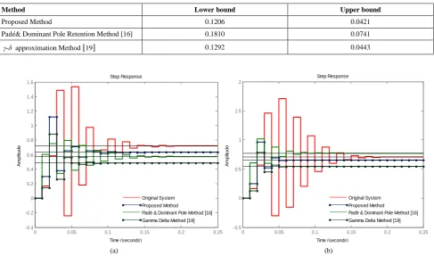
TABLEI. COMPARISONOFISEFORREDUCEDORDERMODELS

Method Lower bound Upper bound

Proposed Method 0.1206 0.0421

Padé& Dominant Pole Retention Method [16] 0.1810 0.0741

γ-δ approximation Method [19] 0.1292 0.0443

I.

Fig. 1. Step response of Original system and reduced systems using Kharitonov’s theorem (a) Fixed transfer function of n1/d1 (b) Fixed transfer

function of n2/d2

The step responses of original uncertain system and reduced order discrete systems using Kharitonov’s theorem are plotted in Fig. 1(a) & 1(b). From Fig. 1(a) & 1(b), it can be observed that step responses of original system and developed reduced order discrete interval system are close to each other, it shows the novelty of proposed method.

0 0.05 0.1 0.15 0.2 0.25

-0.4 -0.2 0 0.2 0.4 0.6 0.8 1 1.2 1.4 1.6

Step Response

Time (seconds)

A

m

p

lit

u

d

e

Original System Proposed Method

Padè & Dominant Pole Method [16] Gamma Delta Method [19]

0 0.05 0.1 0.15 0.2 0.25

-0.5 0 0.5 1 1.5 2

Step Response

Time (seconds)

A

m

p

lit

u

d

e

Original System Proposed Method

Padè & Dominant Pole Method [16] Gamma Delta Method [19]

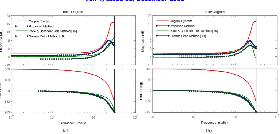
Fig. 2 Frequency response of Original and reduced systems using Kharitonov’s theorem (a) Fixed transfer function of n1/d1 (b) Fixed transfer

function of n2/d2

The frequency response plots for higher order uncertain model and approximate reduced order uncertain model are given in Fig. 2(a) & 2(b). From Fig. 2(a) & 2(b), it can be observed that frequency responses of original system and developed reduced order discrete interval system are close to each other, it shows the novelty of proposed method.

VI. CONCLUSION

This paper discusses an extension of Krishnamurthy & Seshadri’s approach [7] for discrete- time interval systems. Direct Routh table truncation method is utilized for calculation of reduced order system. The proposed technique is easily computable and provides better approximation of higher order discrete system. Lower value of integral square error is associated with developed method produces lower values of when compared with other existing techniques [16, 19].

REFERENCES

[1] Aoki, M., ―Control of large-scale dynamic systems by aggregation,‖IEEE Trans. Automat. Contr., vol. AC-13, pp. 246-253, 1968.

[2] Shamash, Y., ―Continued fraction methods for the reduction of linear time-invariant systems,‖ in Proc. Conf. Cornputer Aided Control

system Design, Cambridge, England,1973, pp. 220-227.

[3] Shich, L. S. and Goldman, M. J., ―A mixed Cauer form for Linear system reduction,‖IEEE Trans. Syst., Man, cybern. vol SMC4, pp. 584-588.

1974.

[4] Chuang, S. C., ―Application of continued-fraction method for modelling transferfunction to give more accurate transient response,‖ Electron.

Lett.,vol6, pp-861-863. 1970.

[5] Shamash, S., ―Stable reduced order models using Padè type approximation,‖IEEE Trans. Automat. Contr., vol. AC-19, pp. 615-616, 1974.

[6] Hutton, M.F., and Friedland, B.,―Routh Approximation for ReducingOrder of Linear Time Invariant System‖, IEEE Trans. Autom.

Control,vol. 20, pp. 329-337, 1975.

[7] Krishnamurthy, V. and Seshadri, V., ―Model Reduction Using the Routh Stability Criterion‖,IEEE Transactions on Autom. Control,vol.

AC-2-3, No. 4, august 1978.

[8] Appiah, R. K., ―Padè methods of Hurwitz polynomial approximation with application to linear system reduction,‖ Int. J. Control, vol. 29, pp.

39–48, 1979.

[9] Chen, T.C., Chang, C.Y., Han, K.W., ―Stable reduced-order Padè approximants using stability equation method,‖ Electron. Lett., vol. 16, pp.

345–346,1980.

-10 -5 0 5 10 15 20

M

a

g

n

it

u

d

e

(

d

B

)

100 101 102 103

-360 -180 0 180 360

P

h

a

s

e

(

d

e

g

)

Bode Diagram

Frequency (rad/s) Original System

Proposed Method

Padè & Dominant Pole Method [16] Gamma Delta Method [19]

-10 -5 0 5 10 15 20

M

a

g

n

it

u

d

e

(

d

B

)

100 101 102 103

-360 -180 0 180 360

P

h

a

s

e

(

d

e

g

)

Bode Diagram

Frequency (rad/s) Original System

Proposed Method

Padè & Dominant Pole Method [16] Gamma Delta Method [19]

[10] Sharma, M., Sachan, A., Kumar, D., "Order reduction of higher order interval systems by stability preservation approach," International conference on Power, Control and Embedded Systems (ICPCES), pp.1-6, 2014.

[11] Shamash, Y., ―Continued Fraction Methods for the Reduction of Discrete Time Dynamic Systems, ‖ International Journal of Control, vol. 20,

p. 267-275, 1974.

[12] Shih, Y. P., Wu, W. T., Chow, H. C., ―Moments of Discrete Systems and Application in Model Reduction, ‖ The Chemical Engineering

Journal, vol. 10, p. 107, 1975.

[13] Parthasarthy, P. and Jayasimha, K. N., ―Modelling of Linear Discrete-Time Systems using Modified Cauer Continued Fraction, ‖Journal of

Franklin Inst, vol. 316, no. 1, p. 79, 1983.

[14] Bandyopadhyay, B., Kande, T.M., Srisailm, M.C., ―Routh Type Approximation for Discrete System, ‖ IEEE International Symposium on

Circuits and Systems, vol.3, 1988.

[15] Kharitonov, V. L., ―Asymptotic stability of an equilibrium position of a family of systems of linear differential equations,‖ Differentsial’nye

Uravneniya, vol. 14, pp. 2086–2088, 1978.

[16] Ismail, O., Bandyopadhyay, B., Gorez, R., ―Discrete interval system reduction using Padé approximation to allow retention of dominant

poles,‖IEEE Trans. on Circuits and Systems-I: Fundamental theory and applications, vol. 44, no. 11, pp. 1075-1078, 1997.

[17] Choo, Y., ―A Note on Discrete Interval System Reduction via Retention of Dominant Poles,‖International Journal of Control, Automation, and

Systems, vol. 5, no. 2, pp. 208-211, 2007.

[18] Singh, V. P. and Chandra, D., ―Model reduction of discrete interval System using dominant poles retention and direct series expansion

method,‖The 5th International Power Engineering and Optimization Conference (PEOCO), pp.27-30,2011.

[19] Choudhary, A. K. and Nagar, S. K., ―Gamma Delta Approximation for Reduction of Discrete Interval System,‖International Joint Conferences

on ARTCom and ARTEE, pp. 91-94, 2013.

[20] Bandyopadhyay, B., Gorez, R., Ismail, O., ―Routh-Padé approximation for discrete interval systems,‖ in Proc. 14th IMACS World Congress

on Computation and Applied Mathematics, Atlanta, GA, vol. 1, pp. 46–48, 1994.