A comparative study of effort estimation techniques using back propagation algorithm

(1)

IJEDRCP1501026

International Journal of Engineering Development and Research (www.ijedr.org)

137

A Comparative Study of Effort Estimation

Techniques Using Back Propagation Algorithm

S. Abbinaya1, M. Senthil Kumar2 1_Student,2_{Associate Professor} Valliammai Engineering College,Chennai

________________________________________________________________________________________________________ Abstract - Software effort estimation is the process of predicting the most realistic amount of effort (expressed in terms of person-hours or money) required to develop or maintain software based on incomplete and uncertain input. Effort estimation is an important part of software development work and provides essential input to project feasibility analyses, bidding, budgeting and planning. This paper is concerned with constructing software effort estimation model based on neural network techniques. In this paper, two common estimation methods like use case point and function point are used to estimate the effort in the software development. The network is trained with the back propagation algorithm by iteratively processing a set of training samples and comparing the two effort estimation methods (use case point and function point) with the actual effort. The performance comparisons of these methods are done by using a sample past project data. Depends upon the requirements, the performance metrics will be changed.

IndexTerms - Artificial neural networks, back propagation, feed forward neural networks, decision table, use case point, function point, software effort estimation, and regression.

________________________________________________________________________________________________________

I.INTRODUCTION

In software engineering effort is used to denote measure of use of workforce and is defined as total time that takes members of a development team to perform a given task. It is usually expressed in units such as man-day, man-month, and man-year. An estimation of accuracy and concise effort (quantity of men/hours required for the development of the software) are crucial for the effective management of the software project [5]. This value is important as it serves as basis for estimating other values relevant for software projects, like cost or total time required to produce a software product. The basic idea of prediction of effort by analogy is that projects having similar features such as size and complexity will be similar with respect to project effort. The method gains its importance since the estimate is based on actual project experience [9].

Traditional algorithmic techniques such as regression models, Software Life Cycle Management (SLIM), COCOMO II model, require estimation process in a long term. But, nowadays that is not acceptable for software developers and companies. Newer soft computing techniques to effort estimation based on non-algorithmic techniques may offer an alternative for solving the problem [4]. The uncertainty in size can be controlled by using fuzzy logic and the parameters can be tuned by using Particle Swarm Optimization. The Fuzzy Based PSO technique is applied for Software Effort Estimation. A methodology is developed to estimate effort using Fuzzy Logic and PSO with inertia weight [1]. But the weights are not updated as in the gradient descent.

Currently used software development effort estimation models such as, COCOMO and Function Point Analysis (FPA), do not consistently provide accurate project cost and effort estimates. These techniques have been proven unsatisfactory for estimating cost and effort because the lines of code (LOC) and function point (FP) are both used for procedural oriented paradigm [6,7]. Both of them have certain limitations. The LOC is dependent on the programming language and the FPA is based on human decisions. Hence effort estimation during early stage of software development life cycle plays a vital role for determining whether a project is feasible in terms of a cost benefit analysis [8].

Accurate estimation of a software development effort is critical for good management decision making. The aim of the present work is to propose an optimal estimation method for software effort estimation. In general software effort estimation, the most commonly adopted architecture, learning algorithm and activation function are the feed-forward multilayer perceptions, the back propagation algorithm respectively [3]. One of the major drawbacks in the existing effort estimation there has been much time spent on the selection of accurate effort estimation. The present work explores a decision table could be developed as a tool which would help on minimizing the time spent on the selection of accurate effort estimation, method and would help organization on, Define most adequate effort estimation method in different software development environment, Implementing the selected technology, Testing of resulting model accuracy.

The remainder of this paper is organized as follows. Section 2 gives an overview of the materials and methods. Section 3 describes the proposed work. Section 4 describes the experimental evaluation. Section 5 concludes and suggests directions for future work.

II.MATERIALS AND METHODS

(2)

IJEDRCP1501026

138

This section gives a brief overview of the steps in the use case point’s method [8]. The first step is to classify the actors as simple, average or complex. A simple actor represents another system with a defined Application Programming Interface, API, an average actor is another system interacting through a protocol such as TCP/IP, and a complex actor may be a person interacting through a GUI or a Web page. A weighting factor is assigned to each actor type in the following manner:

 Simple: Weighting factor 1  Average: Weighting factor 2  Complex: Weighting factor 3

Similarly each use case is defined as simple, average or complex, depending on number of transactions in the use case description, including secondary scenarios. Use case complexity is then defined and weighted in the following manner:

 Simple: Weighting factor 5  Average: Weighting factor 10  Complex: Weighting factor 15

The Calculation of UUCW AND UAW Weights and Points are as follows: UUCP = UAW + UUCW (1)

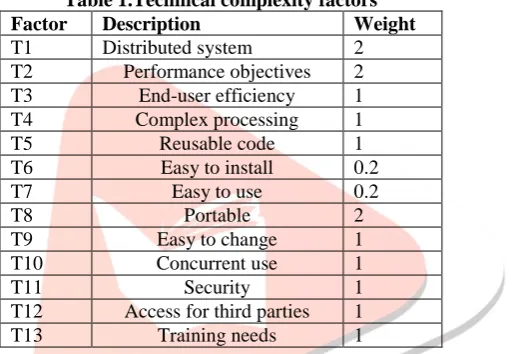
3. The use case points are adjusted based on the values assigned to a number of technical factors (Table 1) and environmental factors (Table 2).

Table 1.Technical complexity factors Factor Description Weight

T1 Distributed system 2

T2 Performance objectives 2

T3 End-user efficiency 1

T4 Complex processing 1

T5 Reusable code 1

T6 Easy to install 0.2

T7 Easy to use 0.2

T8 Portable 2

T9 Easy to change 1

T10 Concurrent use 1

T11 Security 1

T12 Access for third parties 1

T13 Training needs 1

Each factor is assigned a value between 0 and 5 depending on its assumed influence on the project. A rating of 0 means the factor is irrelevant for this project; 5 mean it is essential.

The Technical Factor (TCF) is calculated multiplying the value of each factor (T1–T13) in Table 1 by its weight and then adding all these numbers to get the sum called the Factor. Finally, the following formula is applied:

TCF = 0.6 + (.01*TFactor) --- (2)

Table 2.Environmental factors

Factor Description Weight

E1 Familiar with the development process 1.5

E2 Application experience 0.5

E3 Object-oriented experience 1

E4 Lead analyst capability 0.5

E5 Motivation 1

E6 Stable requirements 2

E7 Part-time staff -1

E8 Difficult programming language -1

4. The Environmental Factor (EF)is calculated accordingly by multiplying the value of each factor (F1 – F8) in Table 2 by its weight and adding all the products to get the sum called the Efactor. The formula below is applied:

EF = 1.4+(-0.03*EFactor) (3) The adjusted use case points (UCP) are calculated as follows:

UCP = UUCP*TCF*EF (4) Function Points Method

(3)

IJEDRCP1501026

139

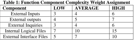
such as Data Element Types (DET), File Types Referenced (FTR) and Record Element Types (RET). Table 1 illustrates how each function component is then assigned a weight according to its complexity. The Unadjusted Function Point (UFP) is calculated with Equation 1, where Wij are the complexity weights and Zij are the counts for each function component.

Table 1: Function Component Complexity Weight Assignment

Component LOW AVERAGE HIGH

External Inputs 3 4 6

External outputs 4 5 7

External Inquiries 3 4 6

Internal Logical Files 7 10 15

External Interface Files 5 7 10

Once calculated, UFP is multiplied by a value Adjustment Factor (VAF), which takes into account the supposed contribution of technical and quality requirements. The VAF is calculated from 14 General System Characteristics (GSC), using Equation 2; The GSC includes the characteristics used to evaluate the overall complexity of the software.

VAF = (TDI * 0.01) + 0.65 (5)

Finally, a FP is calculated by the multiplication of UFP and VAF, as expressed in Equation 3. FP = UFP * VAF (6)

Decision table

 When building a DT, first step is the identification of the conditions and actions and their associated states that have an influence on the decision problem.

 The actual construction of the DT on the basis of the defined decision rules.

 Examines the DT with regard to the requirements of completeness, contradiction and correctness.

 The neural network is used to train the decision table with the previous project effort values. The multilayer feed forward network is used for creating neural network and it has one input layer, at least one hidden layer and one output layer. Back propagation is used as the training methodology i.e. the learning rule.

Neural network

Artificial intelligence (AI) has been widely used in many domains such as medicine, economics, business, and others. Recently, the interest of applying AI in software engineering has been soaring. Conducting software estimation is essential in any project as it helps project managers plan, identify risks, and determine the effort and cost of projects [2]. Artificial intelligence is trying to achieve using techniques like mimicking neural networks.

Computational models inspired by central nervous systems, which is capable of machine learning as well as pattern recognition. Interconnected neurons which can compute values from inputs. The network trained back propagation learning algorithm by iteratively processing a set of training samples and comparing the networks prediction with actual effort.

Back propagation, "backward propagation of errors", is a common method of training artificial neural networks used in conjunction with an optimization method such as gradient descent. The method calculates the gradient of a loss function with respects to all the weights in the network. The gradient is fed to the optimization method which in turn uses it to update the weights, in an attempt to minimize the loss function. The most widely used algorithm for supervised learning with multilayered feed forward networks. The basic idea of back propagation is the repeated application of the chain rule to compute the influence of each weight on the network with respect to an arbitrary error function E [3].

Back propagation requires a known, desired output for each input value in order to calculate the loss function gradient. It is therefore usually considered to be a supervised learning method, although it is also used in some unsupervised networks such as auto encoders. It is a generalization of the delta rule to multi-layered feed forward networks, made possible by using the chain rule to iteratively compute gradients for each layer. Back propagation requires that the activation function used by the artificial neurons (or "nodes") be differentiable.

III.PROPOSED WORK

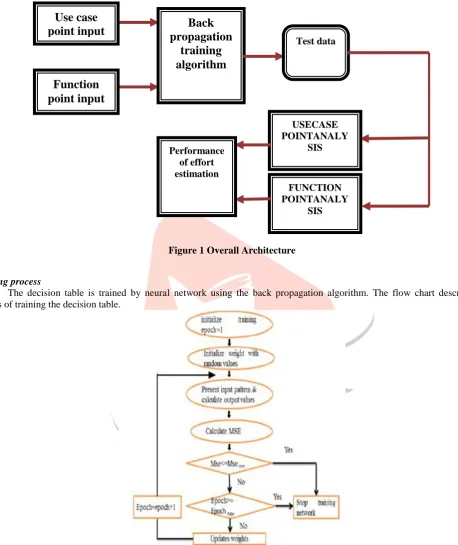
The Architecture diagram shows the overall concept of system. Figure 1 shows the proposed system is devised by using use case point and function point method for estimation. The input of the use case point and function point should be trained by the neural network training algorithm and the trained input is stored in the decision table. To estimating with use case points is that the process can be automated.

(4)

IJEDRCP1501026

140

By using the regression analysis the inputs of those methods will be refined from the trained input. After refined the input, the effort is calculated by two methods i.e. use case point and function point. Finally compare the performance of both estimation methods and the decision table will show which method will produce the accurate result.

Figure 1 Overall Architecture

Training process

The decision table is trained by neural network using the back propagation algorithm. The flow chart describes the process of training the decision table.

Figure 2 Training process flowchart

Initially the value of training iteration is assigned as 1 and the weight with random values. Then present input pattern and calculate the output values. After the output values are calculated, the mean square error (MRE) will be calculated. Then if the calculated MSE is lesser than or equal to the Msemm, the training process will be stopped. Otherwise, the number of iterations will be compared with the maximum number of iterations. If the iteration is greater than or equal to the Epoch max, the training process will be stopped. Otherwise the weights will be updated and the iteration is incremented.

Back

propagation

training

algorithm

Test data

USECASE POINTANALY

SIS

FUNCTION POINTANALY

SIS Performance

of effort estimation

Use case

point input

(5)

IJEDRCP1501026

141

IV.EXPERIMENTAL EVALUATION

The experimental evaluation of the proposed model is performed using 12 projects. In software estimation, most practitioners use MMRE and PRED(X) to calculate the error percentage. The magnitude of relative error (MRE) for each observation I can be obtained as:

│actual efforti– predicted efforti│ MREi =

Actual efforti--- (7)

MMRE can be achieved through averaging the summation of MRE over N observations: MMRE= I --- (8)

On the other hand, PRED(X) is the percentage of projects for which the estimate falls within x% of the actual value. For instance, if PRED (30) = 60, this indicates that 60% of the projects fall within 30% error range.

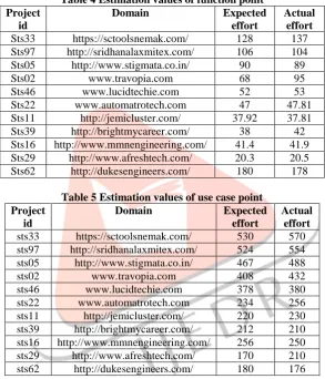
Table 4 Estimation values of function point Project

id

Domain Expected

effort

Actual effort

Sts33 https://sctoolsnemak.com/ 128 137

Sts97 http://sridhanalaxmitex.com/ 106 104

Sts05 http://www.stigmata.co.in/ 90 89

Sts02 www.travopia.com 68 95

Sts46 www.lucidtechie.com 52 53

Sts22 www.automatrotech.com 47 47.81

Sts11 http://jemicluster.com/ 37.92 37.81

Sts39 http://brightmycareer.com/ 38 42

Sts16 http://www.mmnengineering.com/ 41.4 41.9 Sts29 http://www.afreshtech.com/ 20.3 20.5

Sts62 http://dukesengineers.com/ 180 178

Table 5 Estimation values of use case point Project

id

Domain Expected

effort

Actual effort sts33 https://sctoolsnemak.com/ 530 570 sts97 http://sridhanalaxmitex.com/ 524 554 sts05 http://www.stigmata.co.in/ 467 488

sts02 www.travopia.com 408 432

sts46 www.lucidtechie.com 378 380

sts22 www.automatrotech.com 234 256

sts11 http://jemicluster.com/ 220 230

sts39 http://brightmycareer.com/ 212 210 sts16 http://www.mmnengineering.com/ 256 250 sts29 http://www.afreshtech.com/ 170 210 sts62 http://dukesengineers.com/ 180 176 EXPERIMENTAL RESULTS

The performance of use case points and function points are compared using decision table based on the back propagation methodology. It is used to train the neural network. A set of input training data and the expected output is created and the network is trained with the training data set. There are multiple iterations the network tries to converge the expected output. Through multiple iterations over the test data, it does by reducing an error function. The error rate is calculated by using back propagation by compare the error rate between the expected and actual effort of both UCP and FP methods. The following table 6 shows the comparison of Effort estimation results.

Table 6 Comparison of Effort estimation results Project

id

Domain UCP

effort

FP effort

sts33 https://sctoolsnemak.com/ 0.0701 0.0656 sts97 http://sridhanalaxmitex.com/ 0.0541 0.0192 sts05 http://www.stigmata.co.in/ 0.0430 0.0112

sts02 www.travopia.com 0.0555 0.2842

sts46 www.lucidtechie.com 0.0052 0.0188

(6)

IJEDRCP1501026

142

sts16 http://www.mmnengineering.com/ 0.024 0.0119

sts29 http://www.afreshtech.com/ 0.1904 0.0097 sts62 http://dukesengineers.com/ 0.0227 0.0112 PERFORMANCE MEASURES

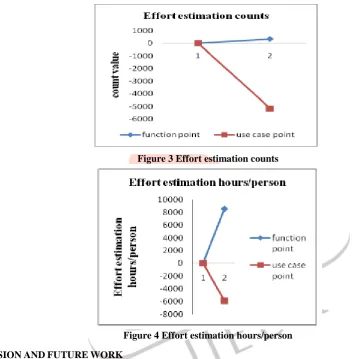
The performance of models generating continuous output can be assessed in many ways, including PRED (30), MMRE, correlation, etc. PRED (30) is a measure calculated from the relative error, or RE, which is the relative size of the differe nce between the actual and estimated value. One way to view these measures is to say that training data contains records with variables 1;2;3;...;N and performance measures add additional new variables N +1;N+2;....

Figure3 and 4 showing the performance chart of both UCP and FP methods

Figure 3 Effort estimation counts

Figure 4 Effort estimation hours/person

V.CONCLUSION AND FUTURE WORK

The use case point (UCP) and function point model has been widely used to estimate software size and effort. The main advantage of the UCP model is that it can be used in the early stages of the software life cycle when the use case diagram is available. The UCP model has some limitations since it assumes that the relationship between software effort and size is linear. There are several software effort forecasting models that can be used in forecasting future software development effort. We have constructed an effort estimation model based on artificial neural networks. The neural network that we have used to predict the software development effort is the single layer feed forward neural network with the identity function at both the input and output units.

In our work we compare the results of two different effort estimation methods and found an optimal neural network topology with best estimation method for software effort estimation. Finally, we conclude that the present work provides accurate forecasts for the software development effort. Further work can be done by the identification and mitigation of risk when estimating the effort. REFERENCES

[1]A.BalaKrishna, T.K.Rama Krishna, fuzzy and swarm intelligence for software effort estimation, Vol. 2, No. 1, ISSN 2167-6372, 2012.

[2] Ali BouNassif and Luiz Fernando Capretz, Danny Ho, Estimating Software Effort Based on Use Case Point Model Using Sugeno Fuzzy Inference System, pages.393-398, 2011.

(7)

IJEDRCP1501026

143

[4] ImanAttarzadeh and Siew Hock Ow,A Novel Algorithmic Cost Estimation Model Based on Soft Computing Technique, Journal of Computer Science 6 (2): 117-125, 2010.

[5] Katia Cristina A. Damaceno Borges, Iris Fabiana de BarcelosTronto, A Data PreProcessing Method for Software Effort Estimation Using Case-Based Reasoning, volume 16, Number 3, 2013.

[6] Mohammed Wajahat Kamal and Moataz A. Ahmed, A Proposed Framework for Use Case Based Effort Estimation using Fuzzy Logic: Building upon the outcomes of a Systematic Literature Review, JNCAA 1(4): 953-976, 2011

[7] OumoutChouseinoglou, A Fuzzy Model of Software Project Effort Estimation, Vol.4, No.2, pp. 68-76, 2013.

[8] ShashankMouliSatapathy, Santanu Kumar Rath, Use Case Point Approach BasedSoftware Effort Estimation using Various Support Vector Regression Kernel Methods, volume7(4),87-101, 2014.

[9] S.Malathi and Dr.S.Sridhar,Estimation of effort in software cost analysis for Heterogeneous dataset using fuzzy analogy, Vol.10, No.10, 2012.