Centre of Policy Studies Working Paper
No. G-251 January 2015
The Implications for Trade and FDI Flows from
Liberalisation of China’s Capital Account
George Verikios
Centre of Policy Studies, Victoria University
ISSN 1 031 9034 ISBN 978-1-921654-59-6
THE IMPLICATIONS FOR TRADE AND FDI FLOWS FROM
LIBERALISATION OF CHINA’S CAPITAL ACCOUNT
George Verikios
Centre of Policy Studies, Victoria University
Abstract
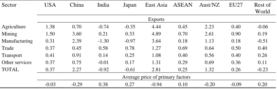
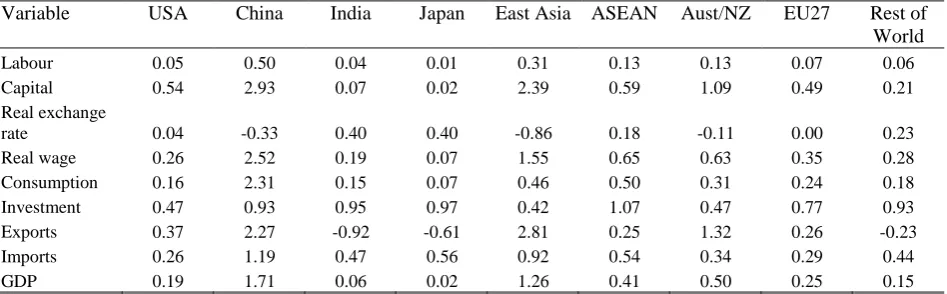
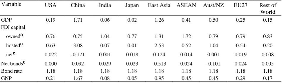
We model the partial liberalisation of the capital account by China using a dynamic CGE model of the world economy. Our results indicate that a reduced capital controls on FDI would lead to a significant increase in FDI capital in China and a significant reduction in the cost of capital in China relative to the rest of the world. Further, we observe an increase in capital stocks in all regions, which benefits all regions in terms of GDP and GNP. The economies of China (1.7%), East Asia (1.3%) and Australia/New Zealand (0.5%) grow most strongly. The rental price of capital falls significantly in these regions, which lowers domestic costs and they experience a real depreciation of the exchange rate and thus increased exports relative to other regions. We also observe an across-the-board increase in the saving rate driven by the rise in the price of consumption relative to investment (saving) in all regions.
JEL codes: C68, E22, F21, F23, F38, F40.
Keywords: capital controls, China, computable general equilibrium, FDI, multinational firms, trade.
Acknowledgements
Table of contents
1. Introduction 1
2. China’s capital account policy 2
3. The model 5
3.1 Production technology 5
3.2 Market clearing and commodity preferences 7
3.3 Regional and sector-specific investment 8
3.4 Aggregate household consumption, government expenditure and saving 9
3.5 Wealth accumulation 10
3.6 Wealth allocation across asset classes 11
3.7 Capital supply across locations and industries 13
3.8 Capital mobility 15
3.9 Labour supply and labour-market clearing 15
3.10 Regional income 16
4. The baseline 17
5. The effects of China partially liberalising the capital account 18
5.1 Capital allocation effects 21
5.2 Trade effects 25
5.3 Macroeconomic effects: GDP 25
5.4 Macroeconomic effects: GNP 26
6. Sensitivity analysis 27
7. Conclusion 28
Tables
1 Values of ro: the elasticity of transformation of capital across locations r
by owner o 15
2 Macroeconomic variables in baseline: 2007-2023 (percentage change) 19
3 Capital allocation effects of partial liberalisation of China’s capital account
(percentage change) 22
4 Rate of return effects of partial liberalisation of China’s capital account
(percentage change) 24
5 Sectoral capital effects of partial liberalisation of China’s capital account
(percentage change) 24
6 Export and primary factor price effects of partial liberalisation of China’s
capital account (percentage change) 25
7 GDP effects of partial liberalisation of China’s capital account
(percentage change) 26
8 GDP and GNP effects of partial liberalisation of China’s capital account
(percentage change) 27
Figures
1 Initial (2013) post-tax net rates of return by location 19
2 An increase in the supply of capital in China 21
3 Responses in real wealth, capital owned and net bonds (percentage change) 23
4 Capital stock response by location to different increases in preferences for
investing in China (percentage change) 28
5 Rate of return response to different increases in preferences for investing
1. Introduction
Two important global macroeconomic policy issues that have emerged since the turn of the
century are exchange rate flexibility and capital account liberalisation by China. Both of these
issues have become more prominent since the Chinese economy became the second largest in the
world in 2010.1 The Chinese authorities have stated publicly that the removal of capital controls
is a medium-term objective (Prasad et al., 2005). There is evidence that the removal of capital
controls by developing countries can have significant macroeconomic effects (Sedik and Sun,
2012). Given this, what might be the likely nature and size of the macroeconomic effects of a
move towards capital account liberalisation by the Chinese authorities? We address this question
by applying an analytical framework that captures the most important macroeconomic features of
this issue as they relate to global foreign direct investment (FDI) and trade.
China’s capital account is tightly controlled (Jeanne, 2012) and the capital controls have
tended to be more restrictive for volatile capital flows (e.g., portfolio investment) compared to
more stable capital flows (e.g., FDI). The controls seem to have initially focused on restricting
outflows but have evolved to manage both inflows and outflows so as to maintain the official
exchange rate (Ma and McCauley, 2007). It is likely that this is a result of an increasing gap,
over time, between the official exchange rate and the likely market exchange rate under a flexible
exchange rate scheme. The large current account surpluses posted by China since 2005 suggest
that the management of inflows has probably been more important than the management of
outflows; this view is supported by the accumulation of enormous foreign exchange reserves by
China.2 If the management of inflows has been the dominant role of capital controls, then this
would have the effect of limiting arbitrage between the (Chinese) domestic cost of capital and
global cost of capital.3 In fact, macroeconomic observers have expressed the view that the capital
controls have had the effect of creating a positive cost of capital differential between the domestic
cost of capital in China and the world cost of capital (Ma and McCaualey, 2010; Prasad and Wei,
2005). There is also evidence that this differential has increased over time (Chen, 2012; Cheung
and Herrala, 2014).
1 This is according to current price data in US$ (IMF, 2014).
2 China’s current account surplus has averaged 4.5% of GDP between 2001 and 2013 (IMF, 2014). China’s foreign
exchange reserves are the world’s largest holdings and are in the order of US$3.8 trillion at the end of 2013 (CIA, 2014).
3 By ‘cost of capital’ we mean the average cost (return) of raising (investing) funds across asset classes, including
Thus, any move to remove or reduce capital controls by China would be expected to lead to
a smaller positive cost of capital differential between China and the rest of the world as FDI and
financial capital would be expected to flow into China from other countries to exploit the
differential. Such inflows are likely to have direct macroeconomic consequences for China: an
increase in the capital stock implying increased investment, in turn, implying higher productivity
and GDP growth in the short-run and permanently higher levels of productivity and GDP in the
long-run. Countries investing in China would likely experience increased income due to
increased investment in China in an attempt to exploit the cost of capital differential. Therefore,
a priori, we would expect capital flows between China and other countries to increase due to the
relaxation of capital controls by China. But, we would also expect an increase in trade flows
between China and other countries as higher GDP growth by China would mean an increased
demand for imports and an increased supply of exports to other countries.
There are no existing studies examining how capital account liberalisation by China would
affect global FDI, trade and other macroeconomic variables. Two related studies quantify the
macroeconomic effects of China’s internal and external policies. Song et al. (2014) use an overlapping generations model of China to analyse the effects of different aspects of China’s
monetary and structural policies, including capital controls, and their interaction with China’s
growth path and other variables. Bénassy-Quéré et al. (2011) use a two-country (China and the
US) overlapping generations model to analyse the interaction of structural reforms under
different policy regimes in China, including the partial liberalisation of capital controls. In both
studies, capital controls are found to be important in determining how China and other economies
react to structural reforms by China. One area to which the current study is distantly related is
the literature on economywide evaluations of removing barriers to trade in services: a major share
of trade in services occurs through FDI (see Christen et al., 2012, for a thorough review of this
literature). These evaluations examine the removal of general or sector-specific barriers to FDI in
China and many other countries, but they do not consider the impact of capital controls, or other
macroeconomic policies, on FDI and trade. Thus, the current work represents a first in
examining the effects of capital account liberalisation by China on global trade and FDI.
2. China’s capital account policy
China has applied capital controls as part of its economic policy since 1949 (Cheung and
China’s high and sustained economic growth since 1980s has slowly increased attention on all
aspects of its economic policies.4 Along with exchange rate flexibility, capital account
liberalisation by China has emerged as an important global macroeconomic policy issue. These
two issues are related but distinct (Prasad et al., 2005).
A move towards exchange rate flexibility and capital account liberalisation has been argued
to pose risks to the Chinese financial sector by allowing outflows from the banking system in
order to exploit foreign investment opportunities. Nevertheless, allowing greater exchange rate
flexibility in the presence of capital controls will not expose China’s underdeveloped financial
system to dangerous risks as Chinese domestic banks are not heavily exposed to currency risk
(Prasad et al., 2005). Furthermore, allowing greater exchange rate flexibility while maintaining
capital controls does not require an immediate move to a freely floating rate (IMF, 2004). In
contrast to the seemingly low risks associated with allowing greater exchange rate flexibility
while maintaining capital controls, there is evidence that liberalising capital controls while
maintaining exchange rate inflexibility has contributed to financial crises in developing
economies (Prasad et al., 2005).
While China’s capital account is tightly controlled (Jeanne, 2012), the capital controls have
tended to be more restrictive for volatile capital flows (e.g., portfolio investment) compared to
more stable capital flows (e.g., FDI). The controls were also initially focused on restricting
outflows, presumably to shield domestic banks from currency risk, but have evolved to manage
both inflows and outflows so as to maintain the official exchange rate (Ma and McCauley, 2007).
Jeanne (2012) and Reinhart and Tashiro (2013) show that control of the capital account (i.e., net
capital inflows) and the official exchange rate (i.e., reserve accumulation) allow the current
account balance to also be tightly controlled. The large current account surpluses posted by
China since 2005 suggest that the management of inflows has probably been more important than
the management of outflows; this view is supported by the accumulation of the world’s largest
holdings foreign exchange reserves. Macroeconomic observers have expressed the view that the
capital controls have had the effect of creating a positive cost of capital differential between the
domestic cost of capital in China and the world cost of capital (Ma and McCaualey, 2010; Prasad
and Wei, 2005).
4 According to current price data in US$, the Chinese economy has grown from being 7% of the size of the US
The Chinese authorities have stated publicly that the removal of capital controls is a
medium-term objective (Cheung and Herrala, 2014; Prasad et al., 2005). Any move to remove or
loosen the capital controls would be expected to lead to the reduction of the positive cost of
capital differential between China and the rest of the world; foreign-sourced loanable funds
within China would increase at the expense of loanable funds in the rest of the world. Given
China’s very high saving rate (around 50%) and its status as the second-largest economy in the
world, it is likely that the removal of capital account controls would also lead to other significant
effects on global capital markets. A freer flow of capital between China and global capital
markets is likely to lead to a substantial repatriation of foreign-currency assets (particular US
dollar assets) held by Chinese residents. Clearly, this will raise yields on US dollar and other
foreign currency assets, and reduce yields on renminbi-denominated assets in China. A freer
flow of capital between China and global capital markets is also likely to lead to a redirection of
funds from non-renminbi assets into renminbi assets in China to exploit their high relative yields.
Both of these effects are will reduce the positive cost of capital differential between China and
the rest of the world.
A smaller cost of capital differential between China and the rest of the world is likely to
lead to direct macroeconomic consequences for China. A lower cost of capital in China, ceterus
paribus, is likely to lead to an increase in the capital stock employed (i.e., capital deepening),
which implies increased investment and faster growth in the capital stock that in turn implies
higher productivity and GDP growth. A lower cost of capital for Chinese households is likely to
lead to a rise in the consumption rate as Chinese households take on debt (or reduce saving) to
increase current consumption and reduce future consumption. A rise in the consumption rate
would be likely to increase imports and reduce exports:5 that is, a reduction in net exports. A fall
in net exports, ceterus paribus, is likely to partially offset GDP growth in China, with the overall
effect of the fall in the cost of capital likely to be positive for China’s GDP growth.
A rise in the world cost of capital would also have implications for nations holding
historically high levels of net foreign debt, e.g., most developed countries, as their servicing
obligations would rise. An increase in servicing obligations would reduce the amount of income
available for both consumption and investment. Lower investment would mean lower growth in
capital and output, ceterus paribus, which would mean lower GDP growth.
The direct macroeconomic consequences described above are likely to have noticeable
impacts on trade flows between China and highly indebted developed countries, but also on other
countries. Beyond this, any fall in loanable funds available to highly indebted developed
economies will also have implications for FDI as these same countries are also the major sources
of FDI (Lakatos and Fukui, 2013). Thus, one way that FDI is financed by these regions is
through foreign debt accumulation, as reflected by large and persistent current account deficits.
If the supply of funds available to these countries decreases, it may mean a rise in FDI by these
regions. If the cost of borrowing to fund all forms of investment rises, this may induce investors
to transfer funds from less risky low return investments (e.g., portfolio investment and sovereign
debt) to more risky high return investments such as FDI.
3. The model
In this study we apply a modified version of the USITC-FDI model (Lakatos and Fukui,
2013). The model represents the global economy within a computable general equilibrium
framework with a focus on FDI, multinational companies differentiated by region of ownership,
and global foreign affiliate data. The model has been modified in order to capture important
elements of modelling liberalisation of China’s capital account. Below we describe the
production and demand structure of the model and the modifications made for this study.
3.1 Production technology
Representative firms are assumed to treat the factors of production (labour and physical
capital) as variable and take factor prices as given in minimising costs. Demands for primary
factors are modelled using nested production functions consisting of two levels. At the top level,
the j (=1,…,6) firms located in the r (=1,..,9) regions and owned by the o (=1,..,9) regions decide
on the (percentage change in) demand for the primary factor composite (i.e., an aggregate of
labour and capital) qFjro using CES (constant elasticities of substitution) production technology: 6
F F
jro jro jro jro
q q p p ; (1)
6 In the formal presentation of the model theory, we use lowercase Latin characters to represent the
where
0.1
is the elasticity of substitution between the primary factor composite andintermediate inputs, qjro is (the percentage change in) the
j r o, ,
-th industry’s activity level,F jr
p is the price of the primary factor composite, and pjro is the price of output by the firm.7
Clearly, equation (1) consists of a scale term
qjro and a substitution term
pFjro pjro
. Thus,with no change in relative prices, changes in output will lead to changes in the demand for the
primary factor composite. With output fixed, changes in relative prices will lead to changes in
the demand for the primary factor composite; this effect will be larger the greater the value of . All of these effects reflect standard optimising behaviour by the firm.
At the second level, firms decide on their demand for the i (=2) factors of production, qijroF ,
again using CES production functions:
F F F F
ijro jro j ijro jro
q q p p ; (2)
where j is the elasticity of factor substitution and 0.5 for all j industries, and F ijro
p is the price
of the i-th primary factor. Like equation (1), equation (2) consists of a scale term and a
substitution term. The value of j is based upon parameter choices that have been extensively
applied in other studies.8
Firms are also assumed to be able to vary the k (=1,…,6) intermediate inputs they use in
production, the prices of which they also take as given in minimising costs. In combining
intermediate inputs, all firms are assumed to use nested production functions. At level 1, all
firms decide on their use of the intermediate input composite qkjroI using CES production
technology;
I I
kjro jro kjro jro
q q p p , (3)
where pkjroI is the price of the i-th intermediate input composite. Equation (3) determines firms’
use of the intermediate input composite as a function of scale and substitution terms.
At level 2, firms decide on their use of individual intermediate inputs from domestic
I
kjro
qd and imported
I
kjro
qm sources also using CES production technology:
7 In describing the production technology, we omit technical change terms to simplify the exposition.
8 See, for example, Adams et al. (2000), Dixon and Rimmer (2002), Dixon et al. (2011), Horridge et al. (2005) and
I I I I
kjro kjro k kjro kjro
qd q pd p , (4)
I I I I
kjro kjro k kjro kjro
qm q pm p , (5)
where I
I
kjro kjro
pd pm is the price of the k-th domestic (imported) intermediate input composite,
and k is the elasticity of substitution between domestic and imported commodities. The values
for the CES at this level range over 2.3–3.3 for traded goods (i.e., agriculture, mining, and
manufacturing), and over 0.1–0.5 for nontraded goods (i.e., services).
All firms are assumed to operate in perfectly competitive markets and so a zero-pure-profits
condition is imposed that equates revenues with costs, which in levels is
. F. F I . I
jro jro jro jro k kjro kjro
P Q P Q
P Q . (6)3.2 Market clearing and commodity preferences
The supply price of the (j,r,o)-th industry
Pjro is linked to the market price
PMKTjro
via PMKTjro Pjro.(1Tjro), where Tjro is the output tax on the (j,r,o)-thindustry. PMKTjro is
determined via a market-clearing condition, which in percentage-change form is
. .
jro jro jro s jros jros
q SD qd
SX qx , (7)where qdjro is domestic sales of the (j,r,o)-th good (i.e., sales to firms, households and
government), qxjros is export sales of the (j,r,o)-th good to region s (=9), and the Ss are the
relevant shares of domestic and export sales in total output.
Domestic sales across firms producing the j-th commodity
qdjro
is determined by CESpreferences as
jro jr j jro jr
qd qd pmkt pmkt , (8)
where qdjr is domestic sales of the j-th good across all firms (i.e., across all owners), and pmjr is
the average market price for good j produced by all firms in region r.
Export sales of the (j,r,o)-th good across the s regions is determined by CES preferences as
jros jr j jros jr
where qmjr is import sales of the j-th good in region r by all agents (i.e., firms, households and
government), and pmjr is the average c.i.f. price for good j imported by region r from all source
regions.
3.3 Regional and sector-specific investment
In original form, USITC-FDI assumes that there is a single investment good available for
all sectors. This assumption is at odds with the assumption of sector-, location- and
owner-specific (physical) capital in the model. Thus, we modify the assumption of a single investment
good by apportioning regional investment across sectors. The apportionment uses capital stock
shares in each region, so the implicit assumption is that investment-capital ratios are equal across
sectors in a region. Once regional investment data has been apportioned across sectors, it is
necessary to determine how sectoral investment will determined in the model.
Sectoral investment by industry j in region r, Ijr, is assumed to be a fixed ratio of sectoral
capital, Kjr, with an adjustment via the shift term FIr;
jr r jr
I
FI
K . (10)
With Ijr determined in (10), industry demands for the k inputs to investment Ikjr are determined
by CES (constant elasticities of substitution) production technology, represented below in
percentage changes;
kjr jr kjr jr
i i pi pi . (11)
where pikjr is the (percentage-change in the) price of the i-th input to investment, pijr is the
(percentage-change in the) average price of inputs to investment. Once Ikjr has been determined,
demands for inputs to investment between domestic and foreign sources is determined by CES
production technology as applied in the original model (see, for example, equations (4)–(5)).
At the top level of the investment technology nest, regional investment Ir is determined as
a share of GDP with an adjustment for the relative rate of return on capital:
.
r r
r r
I ROR
FG
GDP ROR
where RORr
ROR
is the post-tax net (of depreciation) rate of return on capital in the r-thregion (globally), δ (=0.5) is a positive parameter, and FGr is a shifter that ensures both sides of
(12) are equal in the initial solution. To ensure consistency between Ir and Ijr, we add an
adding up constraint:
r j jr
I
I . (13)To ensure that equation (13) is consistent with equations (10) and (12), FIr in (10) is set as
endogenous.
3.4 Aggregate household consumption, government expenditure and saving
The USITC-FDI model follows the GTAP model (Hertel and Tsigas, 1997) by allocating
net (of depreciation) national income across aggregate government consumption, aggregate
household consumption and net (of depreciation) saving to maximise a Cobb-Douglas utility
function with variable scale and share parameters. Therefore, the nominal values of aggregate
government consumption, aggregate household consumption and net (of depreciation) saving are
almost fixed shares of nominal net national income. This treatment of household consumption is
at odds with the life-cycle theory of consumption and saving, which predicts that changes in real
wealth will influence household aggregate spending over and above any changes in current
income or other factors. The policy issue analysed in this work is expected to lead to significant
changes in real wealth, and in order to capture the effects of these changes on household
consumption we implement a life-cycle theory of consumption and saving.
Following Dornbusch and Fisher (1978, pp. 141–54), we assume aggregate nominal
household expenditure (C) in a region moves with nominal household disposable income9 (HDY)
and real wealth (RW):
. .
.C APC HDY RW FD, (14)
where APC is the average propensity to consume out of HDY, α (=0.06) is a positive parameter
that controls the average propensity to consume out of real wealth, and FD is scaling factor that
ensures that both sides of (14) are equal in the initial solution.
The above treatment of household consumption replaces the original treatment in
USITC-FDI, which also affects the treatment of government consumption and saving. Government
consumption (G)is now assumed to be a fixed share of GDP, in nominal terms. Thus, saving (S)
is now a residual, being the difference between GNP, or national income, and household
consumption and government consumption. This means that the saving rate, S/GNP, is
endogenous and is determined by equation (14), i.e., 1 –(C + G)/GNP.
3.5 Wealth accumulation
The USITC-FDI model is comparative-static. As we wish to be able to use the model in
dynamic form, i.e., apply the model to forecast the evolution of each region’s economy from
today to some period in the future, we add dynamics to the model in the form of wealth
accumulation. The derivation of the wealth accumulation mechanism and its explanation follows
Dixon and Rimmer (2002, pp. 43–7).
In applying the model in dynamic form, we can simulate the evolution of regional and
global economies between two points in time, e.g., 2013-2023. With such a simulation, there is
only a single time period but its length is 10 years. Thus, any accumulation relationship over this
10-year period requires an assumption about how model variables evolve through the simulation
period. Following Dixon and Rimmer (2002), we assume model variables growth smoothly over
the period. This means that stock and flow values from 2013 are treated as parameters in the
model and those for 2023 are treated as variables. Thus, we assume that each region’s wealth
accumulates over the period as:
1
t s t s t s
W W NS , s0,1,...,9. (15)
where Wt is the value of wealth at the beginning of year t, and NSt is the value of net (of
depreciation) saving during year t.
Equation (15) says that wealth at the beginning of year t+s+1 equals wealth at the
beginning of the previous year plus net saving during year t+s. Equation (15) can be written in
terms of Wt as
1
0
t t s t s
W W NS
. (16)Now assume that net saving grows smoothly over the simulation period, i.e.,
.
s t t s t
t
NS
NS NS
NS
. (17)
1
0 .
s t
t t s t
t
NS
W W NS FW
NS
, (18)where FW is a variable representing the preference for wealth accumulation. Note that Wt and
t
NS in (18) are parameters and set to values from 2013.10
3.6 Wealth allocation across asset classes
We define wealth for each regional investor as consisting of two assets: physical capital and
bonds. Physical capital (K) is already defined in USITC-FDI by industry j, location r, and owner
o: Kjro, where the location and owner dimensions refer to regions in the model. In allocating
wealth between physical capital and bonds, the choice refers to total capital owned by owner o:
o j r jro
K
K .Here, bonds (B) represent all forms of debt and equity financing, i.e., all financial assets
and liabilities.11 Thus, bonds are calibrated for each region so they represent net foreign income
on all assets other than physical capital; this is achieved by setting regional net income from
bonds so that the capital account balance matches observed values.12 In this way, bonds (i) allow
the capital account to be closed, (ii) give investors a choice of two types of assets in which to
invest their saving, with bonds representing a lower risk investment, and typically a lower return
investment, than FDI. The inclusion of bonds thus represents investor choices and global capital
markets more realistically than would otherwise be the case. As bonds represent a composite of
all financial assets, they are modelled as net stocks for each region.
10 One flaw in (18) is that it does not accord with 2013 values of wealth and net saving. That is, (18) is not an initial
solution given the starting values (i.e., the values in 2013) of wealth and net saving. If all t+τ (2023) values in (18) are replaced with t (2013) values, then the left-hand side (LHS) of (18) equals Wt but the right-hand side (RHS) equals WtNSt: the LHS and the RHS are not equal to each other. This flaw is overcome by adding to (18) the term NSt. 1 U, where U = 0 in the initial solution and U = 1 in the final solution. In the modified form of (18), if all t+τ (2023) values are replaced with t (2013) values, both the LHS and the RHS equal Wt. Setting U = 1 in the final solution imposes the original relationship in (18).
11 This treatment of bonds is originally due to McDougall (1993) but its application here more closely follows
Hanslow et al. (1999).
In allocating wealth between physical capital and bonds, each regional investor chooses Ko
and Bo so as to maximise
K RKo. oVDoB RBo.
subject to QWo CET K B
o, o
,13 whereCET[.] is a constant elasticity of transformation utility function (Powell and Gruen, 1968), RKo
is the average post-tax rental price of capital received by investor o, RB is the global bond rate,
and QWo is real wealth of investor o. o jro. jr. jr
jr
VD
K PI D : i.e., the value of depreciation ofcapital owned by investor o, where Djr is the depreciation rate on capital used by industry j in
region r.
Thus, investors seek to maximise returns on wealth, which comprises (i) post-tax returns on
capital net of depreciation
K RKo. oVDo
, plus (ii) returns on bonds
B RBo.
, given RKo, PIjrand RB. Note that returns on bonds could be positive or negative depending on the initial value
of B: thus o 0
oB
. Note also that there is only a single bond rate as we assume perfect international arbitrage in the bond rate.The maximisation problem for investors yields the following behavioural equations in
percentage-change form:
o o o o o
k qw ror rorw fk , (19)
.
o o o o o
qb qw CD rbrorw fb ; (20)
where ko
qbo is the quantity of capital (bonds) owned by region o, roro is the post-tax net (ofdepreciation) rate of return on capital in region o, and rorwo is the average rate of return on
wealth in region o.
1.5
is a negative parameter controlling the degree of transformation between capital and bonds. fko and fbo are terms representing preferences to hold wealth in theform capital and bonds.
Equations (19)–(20) comprise scale and transformation terms. The scale term is
determined by real wealth in region o
qwo
: this is nominal wealth
wo deflated by a wealthprice index. The transformation terms are a function of the relative rate of return of each asset
class and the transformation parameter. Note the coefficient CDo for the equation determining
13 As
o
B can take a negative value, the representation of the constraint as QWoCET K B
o, o
is not strictlythe quantity of bonds. CDo 1 for Bo 0 and CDo 1 for Bo 0; for no region is Bo 0.
This coefficient makes qbo rise (fall) with
rbrorwo
if a region is a net creditor (debtor), i.e.,they will lend (borrow) more (less).
3.7 Capital supply across locations and industries
Once capital by owner
Ko has been determined at the top level of the asset supply nest, itremains for capital to be allocated across the r regional locations and the j industries within those
locations: Kjro. It is common for a CET utility function to be applied in determining Kjro given
o
K in models designed to analyse FDI, e.g., Hanslow et al. (1999). But as Hanslow (2001)
demonstrates, if the (j,r)-th capital stock share, Kjro Ko, is small in the initial data, then this
share will stay small as long the (j,r)-th relative rate of return is approximately constant; this is
true regardless of how other rates of return are changing. Therefore, if all capital suppliers to the
(j,r)-th market experience the same change in their relative rates of return, the large suppliers will
remain large and the small suppliers will remain small. To avoid this property of the CET
function, we follow Hanslow (2001) in applying a modified form of the CRETH (constant ratios
of elasticities of transformation, homothetic) utility function (Vincent et al., 1980) to determine
the bilateral allocation of capital across industries.
Thus, in allocating Ko across locations and industries, each regional owner of physical
capital chooses Kjro so as to maximise jro. jro jro
jrK RK VD
subject to Ko CRETH K jro,where RKjro is average post-tax rental price of capital received by investor o.
. .
jro jro jr jr
VD K PI D : i.e., the value of depreciation of capital owned by investor o used by
industry j in region r. Thus, investors maximise returns on total physical capital they own given
jro
RK and PIjr.
The maximisation problem for capital investors yields the following behavioural equations
in percentage-change form:
*
jro o ro jro o jro
k k ror ror fk , (21)
where rorjro is the post-tax net (of depreciation) rate of return on capital owned by region o,used
by region o calculated using special shares (see below), and ro is a negative parameter
controlling the degree of transformation across industries and industries. fkjro represents
preferences to hold capital across industries and locations.
In levels, *
o
ror is defined as
* * * * * o o o o o VPR VD ROR VK VK
. (22)
The first term on the right-hand side (RHS) of (22) is the gross rate of return on capital, that is,
the ratio of post-tax rentals to the capital stock; the second term is the depreciation rate, that is,
the ratio of the value of depreciation to the value of the capital stock. All variables on the RHS of
(22) are calculated using ‘modified’ shares. For example, o* ro* jro. jr
r j
VK
S K PI where* . . ro ro ro ro ro r VK S VK
.The CRETH specification allows the elasticity of transformation, ro, to vary across the r
locations where the o regions invest. Hanslow (2001) calibrates ro so that the values are
inversely related to the initial capital rental shares; this avoids the property described above when
applying CET functions whereby small initial capital shares stay small if the relative rate of
return is constant. Thus, following Hanslow (2001), ro is calibrated as
1
. N
ro o Sro
, (23)
where
2 1 1
2
1 1 2 2
. 1 ro . ro N
r r o N N ro ro r r S S S S
, (24). . jro jro j ro jro jro r j K RK S K RK
. (25)The parameter μ is the average transformation elasticity desired by the model user over all r for
jro
K ; in this case μ = -1. The shares in (25) are post-tax rental shares across locations r for each
investor o. The scheme in (23)–(25) yields CRETH parameters that are inversely related to the
initial rental shares. N controls the standard deviation of the parameters across locations for each
investor given a mean of μ. Higher values of N yield a smaller standard deviation and vice versa.
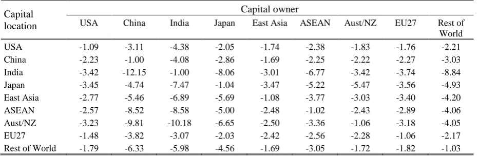
Table 1. Values of ro: the elasticity of transformation of capital across locations r by owner o
Capital location
Capital owner
USA China India Japan East Asia ASEAN Aust/NZ EU27 Rest of World USA -1.09 -3.11 -4.38 -2.05 -1.74 -2.38 -1.83 -1.76 -2.21 China -2.23 -1.00 -4.08 -2.86 -1.69 -2.25 -2.22 -2.27 -3.03 India -3.42 -12.15 -1.00 -8.06 -3.01 -6.77 -3.42 -3.74 -8.84 Japan -3.45 -4.74 -7.47 -1.04 -3.47 -5.22 -5.47 -3.56 -4.93 East Asia -2.77 -5.46 -6.89 -5.69 -1.08 -3.77 -3.03 -3.40 -4.20 ASEAN -2.57 -8.52 -8.58 -5.00 -2.48 -1.02 -2.43 -2.89 -4.06 Aust/NZ -3.23 -9.81 -10.18 -6.65 -2.50 -3.36 -1.06 -3.18 -4.05 EU27 -1.48 -3.82 -3.07 -2.03 -2.42 -2.56 -2.28 -1.06 -2.17 Rest of World -1.79 -6.33 -5.98 -4.56 -1.69 -3.05 -1.72 -1.82 -1.03
Source: See text for explanation.
3.8 Capital mobility
Having determined Kjro, we define capital supply by industry j in region r across all
owners: jr jro. jro
o
K
S K . We also define capital demand by industry j in region r across allowners: QKjr
oSijroF .QijroF , i (= capital). By declaring a market-clearing condition by industryand region, Kjr QKjr, we define a rental price of capital that is common to all owners of capital
in the (j,r)-th industry: PjrK. Thus, any change that causes a fall in the price of capital for any
supplier of capital to the (j,r)-th industry will reduce the price of capital for all owners of capital
in the (j,r)-th industry. For example, if a supplier or group of suppliers increase their supply of
capital to a given regional industry relative to the demand for capital, then all other suppliers of
capital to the industry will experience a fall in their rental price. In this way, any cost-reducing
technical change experienced by one capital supplier is transferred to all other suppliers in the
same regional industry.
Consistent with this treatment of rental prices by industry, in the initial data we set net rates
of return to capital to be equal across all suppliers of capital to a regional industry. Thus, rates of
return vary across industries within a region, but they do not vary across owners of capital within
the same industry in a region.
3.9 Labour supply and labour-market clearing
We define a labour supply function in each region as a function of population and the
evidence on non-zero wage elasticities of labour supply (e.g., Bargain et al., 2011). Thus, in each
region r we define the ratio of the labour supply LSr to population POPr as
.r
r r
r
LS
PRW A
POP
; (26)
where PRWr is the post-tax real wage received by labour in region r and Ar and β are positive
parameters. Thus, labour supply is a positive function of the real wage and population. We set
the labour supply elasticity β = 0.2, making labour supply only slightly responsive to real wage in
each region. Ar is a scaling factor that is set to ensure equality between each side of (26) in the
initial solution of the model.
In original form USITC-FDI assumes the aggregate demand of labour in each region LDr
is exogenous. With LSr now defined in (26), we make LDr endogenous and add the
labour-market-clearing condition
lr lr
LS LD . (27)
Equation (27) now determines the pre-tax wage received by labour in region r Wr by equating
labour demand and supply.
3.10 Regional income
With each region earning foreign income it is necessary to redefine regional income to
reflect the difference between economic activity within a region, i.e., GDP, and income earned by
the region, i.e., GNP. GDP in location r from the supply side and the demand side is defined as
r r r r r r r r r
GDP LY KY IT C I G X M , (28)
i.e., the sum of labour income
LYr , capital income
KYr
and indirect tax receipts
ITrequals the sum of consumption
Cr , investment
Ir , government expenditure
Gr and nextexports
XrMr
. Note that KYr
j oKYjro: KYr includes capital income earned in theall industries by all investors. Also note that ro jro
j
KY
KY for r = o is capital income earnedon domestically-owned capital in region r, and ro jro
j
KY
KY for r ≠ o is capital incomeearned on foreign-owned (or FDI) capital in region r.
r r r r r
GNP GDPFKY FKP NINT . (29)
That is, GDP plus capital income on FDI received by region r
FKYr
, minus capital incomepaid on FDI in region r
FKPr
, plus net interest receipts on bonds for region r
NINTr
.4. The baseline
The USITC-FDI model data is based on version 8 of the GTAP database that represents the
world economy in 2007. In order simulate the policy change from a more recent representation
of the world economy, we update the model database to the most recent year for which historical
data is available: 2013. This is the first step of the baseline. The second step of the baseline is to
forecast the model into future.
Step 1
Model variables are updated from 2007 to 2013 by applying observed movements in GDP,
population, consumer prices, and saving and investment ratios to GDP.14 The historical data is
taken from the IMF’s World Economic Outlook publication.15 The objective of this step is to
ensure the model data conforms approximately to the pattern of global economic activity in 2013.
Therefore, this step is not intended to strictly represent historical movements in global economic
activity but to ensure we have a representation of the global economy in 2013 that conforms
approximately to independent sources (i.e., the IMF), and to use that representation to conduct
the policy simulations.
The following assumptions are made in applying this step:
employment is assumed to be determined by market-clearing between the demand and
supply of labour in each region: see equation (27);
regional saving-to-GDP ratios are targeted via accommodating movements in the average
propensity to consume (APC): see equation (14);
regional investment-to-GDP ratios are targeted via accommodating movements in
preferences for investing (FGr): see equation (12);
14 The model is implemented and solved using the GEMPACK economic modelling software (Harrison and Pearson,
1996).
regional GDP is targeted via accommodating movements in labour-saving technical change;
rates of return on capital are held fixed via accommodating movements in preferences for
wealth accumulation (FW): see equation (18);
The last two assumptions allow capital-output ratios to remain approximately constant, which
accords with historical observation (Romer, 2001, p. 26).
Step 2
The model is then projected forward by 10 years to 2023 using IMF forecasts for GDP,
population and consumer prices. The following assumptions are made in applying this step:
employment is assumed to be determined by market-clearing between the demand and
supply of labour in each region: see equation (27);
household consumption is a function of disposable household income and real wealth: see
equation (14);
investment is a function of GDP and the rate of return on capital: see equation (12);
regional GDP targets are achieved via accommodating movements in labour-saving
technical change;
rates of return on capital are held fixed via accommodating movements in preferences for
wealth accumulation: see equation (18);
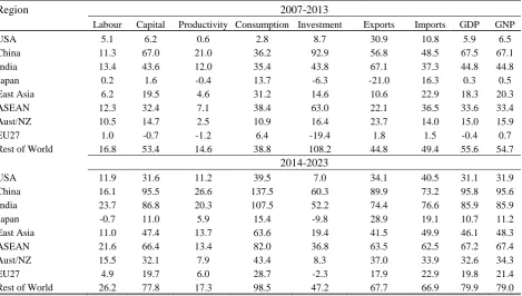
Table 2 presents the changes in real macro aggregates for steps 1 and 2 of the baseline.
5. The effects of China partially liberalising the capital account
The literature review in Section 2 described that macroeconomic observers have expressed
the view that China’s capital account controls have had the effect of creating a positive cost of
capital differential between China and the rest of the world. The initial rates of return for 2013 in
our model are consistent with this view. Figure 1 shows that the global average rate of return is
around 9% whereas in China it is around 14%; so there is a 5 percentage point gap between the
rate of return in China and the global average. Figure 1 also shows that high-income countries
with open capital accounts and flexible exchange rates have the lowest rates of return: USA,
Table 2. Macroeconomic variables in baseline: 2007-2023 (percentage change)
Region 2007-2013
Labour Capital Productivity Consumption Investment Exports Imports GDP GNP
USA 5.1 6.2 0.6 2.8 8.7 30.9 10.8 5.9 6.5
China 11.3 67.0 21.0 36.2 92.9 56.8 48.5 67.5 67.1
India 13.4 43.6 12.0 35.4 43.8 67.1 37.3 44.8 44.8
Japan 0.2 1.6 -0.4 13.7 -6.3 -21.0 16.3 0.3 0.5
East Asia 6.2 19.5 4.6 31.2 14.6 10.6 22.9 18.3 20.3
ASEAN 12.3 32.4 7.1 38.4 63.0 22.1 36.5 33.6 33.4
Aust/NZ 10.5 14.7 2.5 10.9 16.4 23.7 14.0 15.0 15.9
EU27 1.0 -0.7 -1.2 6.4 -19.4 1.8 1.5 -0.4 0.7
Rest of World 16.8 53.4 14.6 38.8 108.2 44.8 49.4 55.6 54.7
2014-2023
USA 11.9 31.6 11.2 39.5 7.0 34.1 40.5 31.1 31.9
China 16.1 95.5 26.6 137.5 60.3 89.9 73.2 95.8 95.6
India 23.7 86.8 20.3 107.5 52.2 74.4 76.6 85.9 85.9
Japan -0.7 11.0 5.9 15.4 -9.8 28.9 19.1 10.7 11.2
East Asia 11.0 47.4 13.7 63.6 19.4 41.5 49.9 46.1 48.3
ASEAN 21.6 66.4 13.4 82.0 36.8 63.5 62.5 67.2 67.4
Aust/NZ 15.5 32.1 7.9 43.4 8.3 37.0 33.9 32.6 34.3
EU27 4.9 19.7 6.0 28.7 -2.3 17.9 22.9 19.8 21.4
Rest of World 26.2 77.8 17.3 98.5 47.2 67.7 66.9 79.9 79.0
Figure 1. Initial (2013) post-tax net rates of return by locationa
0.049
0.144
0.164
0.050
0.104 0.157
0.059 0.071
0.136
0.089
0.00 0.05 0.10 0.15 0.20
USA China India Japan EAsia ASEAN AusNz EU27 ROW World
a This is the ratio of capital rentals (after-tax) to the capital stock minus the depreciation rate.
A priori, partial or complete removal of capital controls by China would be expected to lead
to an influx of FDI and other capital with the intention of exploiting the high relative rate of
return. The literature discussed in Section 2 supports the idea that capital controls have restricted
inflows more that outflows. Such an influx would reduce the gap between the rate of return in
China and the global average. Further, as we assume that the rental price of capital in each
China will reduce the rate of return for all suppliers of capital in each industry, including
domestic suppliers. In this way, increased FDI automatically brings with it benefits to the
domestic industry in terms of a lower cost of capital and higher productivity.
The literature provides little guidance on the degree to which the rate of return in China
would fall relative to the global average by partial or complete removal of capital controls by
China. Nevertheless, we would not expect the complete elimination of the rate of return gap even
with complete capital liberalisation, as the relatively high rates of return in China would reflect
more than just the tightly controlled capital account. For instance, although China’s economy is
the second largest in the world its GDP per capita is still less than some developing countries,
e.g., Mexico. Given this relatively low level of output per capita, one would expect that there
would still be many unexploited investment opportunities in such an economy, and this would be
consistent with high relative rates of returns. Thus, we would expect only a partial elimination of
the gap between rates of return in China and globally even with the complete removal of capital
controls in China. From a political economy perspective, the literature does suggest that
complete capital account liberalisation by China is unlikely in the medium term unless it also
abandons nominal exchange rate targeting.
Given the above discussion, we simulate the partial liberalisation of China’s capital account
by increasing the preference for other countries to locate FDI in China. This is the variable fkjro
in equation (21) (the capital supply function). Capital controls are non-tariff barriers and, as
such, we model their reduction by increasing the preference for all regions to invest FDI in China
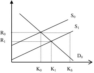
at initial rates of return. This is equivalent to an outward shift of the supply curve for capital in
China (see Figure 2). The initial equilibrium is at the intersection of S0 and D0 giving an initial
rental price of R0 and capital stock of K0. We model the removal of capital controls in China as
they relate to FDI as a shift from S0 to S1, representing an increased preference to invest in China
by the distance KS–K0. As drawn in in Figure 2, this would lead to a fall in the rental price to R1
and an increase in the capital stock to K1. Thus, our simulations should show a fall in the rate of
Figure 2. An increase in the supply of capital in China
Initially we increase the preference to invest in China at initial rates of return by 50% in
order to observe the pattern of effects we might observe. Subsequently we simulate preference
increases of 100% and 200%. In all our simulations we observe a reduction in the rate of return
in China relative to the global average: larger increases in preferences lead to larger reductions in
the rate of return in China relative to the global average.
5.1 Capital allocation effects
Table 3 shows how the allocation of capital across locations and owners is affected by the
policy change; note that diagonal cells represent domestically-owned capital and off-diagonal
cells represent FDI capital. All regions increase their (FDI) capital in China with the biggest
increases by East Asia (17%), Aust/NZ (13%), USA (13%) and EU27 (12%). In general, the size
of the response for each region reflects how much capital they initially have invested in China:
East Asia, USA and EU27 are the biggest foreign owners of capital in China. Australia’s strong
response is driven by the strong trade benefit it derives from the policy change (this is explained
later). As predicted by the partial-equilibrium analysis of Figure 2, the responses by regions
investing in China are less than the increase in preferences for investing in China (50%) as
increasing FDI in China reduces the rate of return earned on such capital (Table 4); this is
consistent with each owner optimising the rate of return on their capital so that, other things being
equal, less FDI capital is allocated to a destination as the rate of return falls.
S0
S1
D0
R0
R1
Table 3. Capital allocation effects of partial liberalisation of China’s capital accounta (percentage change)
Capital location
Capital owner
USA China India Japan East Asia ASEAN Aust/NZ EU27 Rest of
World TOTAL b
USA 0.5 1.1 0.0 -0.1 2.4 0.5 1.3 0.4 0.1 0.5
China 13.2 1.7 6.9 9.3 17.4 11.7 13.1 12.4 8.7 2.9
India 1.3 1.5 0.0 0.1 3.6 0.7 1.9 0.8 0.3 0.1
Japan 0.9 1.1 0.1 0.0 2.7 0.6 1.5 0.7 0.2 0.0
East Asia 1.3 0.9 -0.3 -0.1 2.5 0.3 2.1 0.6 -0.1 2.4
ASEAN 1.3 1.6 0.2 0.2 3.5 0.5 1.7 0.8 0.2 0.6
Aust/NZ 0.9 0.9 -0.1 -0.1 2.7 0.3 1.1 0.5 -0.1 1.1
EU27 0.8 1.1 0.0 0.0 2.7 0.4 1.4 0.5 0.1 0.5
Rest of World 1.0 1.5 0.2 0.1 3.1 0.7 1.6 0.7 0.1 0.2
TOTALc -0.2 1.7 0.0 -0.2 0.7 0.0 0.5 -0.1 0.0 0.7
Source: Model simulation. a Diagonal cells represent domestically-owned and located capital and off-diagonal cells represent FDI capital. b Row totals represent total capital located in region r: this is capital owned and located in region r plus foreign-owned capital located in region r. c Column totals represent total capital owned by region r: this is capital owned and located in region r plus capital owned by region r but located in other regions.
The policy change leads to an increase in capital located in almost all regions (Table 3, last
column). The total capital stock located in China (i.e., domestic- and foreign-owned) rises by
2.9%. Most other regions experience much smaller increases in the total capital stock except for
East Asia (2.4%). East Asia benefits greatly from the policy change and thus grows strongly.
This leads to a larger expansion in domestically-owned capital in East Asia (2.5%) than in
foreign-owned capital (0.9%), i.e., the share of foreign-owned capital falls; this is not the case in
most other regions.
Although the policy change leads to a noticeable increase in capital located in all regions it
does not lead to an increase in capital owned by all regions (Table 3, last row); USA, India,
Japan, ASEAN, EU27 and the Rest of World experience either a minor reduction or a minor
increase in the capital they own. Despite this, global capital rises by 0.7%. Physical capital and
bonds represent the two asset classes owned by a region, and together they constitute wealth by
region. Figure 3 shows that, in general, capital owned moves with real wealth due to the policy
change. East Asia and Aust/NZ are two notable exceptions to this pattern. In both of these
regions, the increases in capital owned are financed by an increase in borrowings (net bonds),16
and the net effect is to lower real wealth. The net effect across all regions is an increase in real
wealth of 0.08%. The wealth accumulation mechanism (equation (18)) is a function of nominal
16 Although it is not obvious in Figure 3, net bonds continue to sum to zero after the reallocation of FDI to China.
net (of depreciation) savings over the period 2013-2023, which rises by about 0.9% globally.
This reflects the rise in gross saving in all regions due to a rise in the saving rate in all regions;
the rise in saving rates is driven by the global rise in the price of consumption relative to the price
of investment: -0.05% cf. -0.005%. The policy change has the effect of increasing the
capital-labour ratio in all regions and thus reducing the price of capital relative to capital-labour. As investment
is more capital intensive than consumption, the price of investment falls relative to the price of
consumption and this encourages households to switch part of their income from consumption to
saving.
Figure 3. Responses in real wealth, capital owned and net bonds
(percentage change)
-2 -1 0 1 2 3 4 5 6 7
USA China India Japan EAsia ASEAN AusNZ EU27 ROW
Real wealth Capital owned Net bonds
The growth in the global capital stock (0.6%) drives down the global rate of return on
capital (-0.8%) (Table 4). Rates of return also fall in all regions where the total capital stock
increases; that is, everywhere except Japan. For all capital owners except India and Japan, the
rate of return on FDI capital invested in most locations also falls reflecting the rise in FDI capital
Table 4. Rate of return effects of partial liberalisation of China’s capital accounta, b (percentage change)
Capital location
Capital owner
USA China India Japan East Asia ASEAN Aust/NZ EU27 Rest of
World TOTAL c
USA -1.2 -1.9 0.1 0.0 -4.1 -0.6 -2.0 -0.9 -0.2 -1.2
China -13.4 -1.7 -7.9 -10.4 -18.2 -13.0 -14.3 -12.9 -10.3 -3.3
India -1.4 -1.7 0.1 0.0 -4.1 -0.7 -2.0 -0.9 -0.2 0.0
Japan -1.6 -1.8 0.1 0.2 -4.5 -0.7 -2.3 -1.0 -0.1 0.1
East Asia -1.4 -1.8 0.0 0.0 -3.6 -0.8 -2.0 -1.0 -0.2 -3.4
ASEAN -1.3 -1.7 0.1 0.0 -4.0 -0.3 -1.9 -0.9 -0.1 -0.4
Aust/NZ -1.5 -1.8 0.1 0.0 -4.4 -0.8 -1.9 -1.0 -0.2 -1.8
EU27 -1.2 -1.9 0.1 0.1 -4.3 -0.7 -2.1 -0.7 -0.1 -0.7
Rest of World -1.2 -1.8 0.1 0.0 -3.7 -0.6 -1.8 -0.8 -0.1 -0.2
TOTALd -1.4 -1.7 0.1 0.1 -4.7 -0.6 -2.0 -0.9 -0.1 -0.9
Source: Model simulation. a The rate of return is defined as the ratio of capital rentals (after-tax) to the capital stock minus the depreciation rate. b Diagonal cells represent the rate of return on domestically-owned capital and off-diagonal cells represent the rate of return on FDI capital. c Row totals represent the average rate of return on total capital located in region r d Column totals represent the average rate of return on total capital owned by region r: this is capital owned and located in region r plus capital owned by region r but located in other regions.
In its initial effect, the policy change does not favour any particular sector in China. Thus,
as reflected in Table 5, capital in each sector expands by similar proportions. However, the
capital stock increases slightly favour mining and manufacturing in China. Mining capital stocks
also grow strongly in other regions where aggregate capital stocks grow strongly (East Asia and
Aust/NZ); this reflects the capital-intensive nature of production of mining. Thus, mining
benefits strongly when the relative price of capital falls in these regions. But unlike China, the
increases in mining capital are driven by mainly by an expansion in domestically-owned capital
rather than FDI capital.
Table 5. Sectoral capital effects of partial liberalisation of China’s capital account (percentage change)
Sector
Location
USA China India Japan East Asia ASEAN Aust/NZ EU27 Rest of World
Agriculture 0.61 2.59 -0.04 -0.26 2.58 0.41 1.22 0.37 0.05
Mining 0.78 3.21 -0.22 -0.32 4.29 0.62 1.96 0.77 0.12
Manufacturing 0.65 3.20 -0.18 -0.31 3.41 0.45 1.38 0.47 0.00
Trade 0.49 2.82 0.10 0.07 2.17 0.67 0.88 0.50 0.24
Transport 0.59 2.47 0.15 0.05 2.24 0.68 1.08 0.53 0.24
Other services 0.51 2.83 0.25 0.10 1.96 0.70 0.93 0.49 0.35