Meander belt delineation: Developing a predictive model for meander belt width

(1)

Western University Western University

Scholarship@Western

Electronic Thesis and Dissertation Repository

9-27-2017 1:00 PM

Meander belt delineation: Developing a predictive model for

meander belt width

Julia Howett

The University of Western Ontario

Supervisor Peter Ashmore

The University of Western Ontario Graduate Program in Geography

A thesis submitted in partial fulfillment of the requirements for the degree in Master of Science © Julia Howett 2017

Follow this and additional works at: https://ir.lib.uwo.ca/etd

Recommended Citation Recommended Citation

Howett, Julia, "Meander belt delineation: Developing a predictive model for meander belt width" (2017). Electronic Thesis and Dissertation Repository. 4915.

https://ir.lib.uwo.ca/etd/4915

This Dissertation/Thesis is brought to you for free and open access by Scholarship@Western. It has been accepted for inclusion in Electronic Thesis and Dissertation Repository by an authorized administrator of

(2)

i

Abstract

The delineation of a meander belt has been recognized in Ontario through land use planning

policies as a primary tool for determining the extent a river or stream requires for natural

meandering tendencies; thus, providing input to channel restoration projects, development

constraints or limits, and regulated areas for species-at-risk. Current delineation procedures utilize

site-specific historical migration assessments, or published empirical equations to predict meander

belt width. In the case of altered, low order watercourses in southern Ontario, the meander belt

width dimension is usually assessed by the application of empirical relations, as the available

historic record often lacks the information necessary to conduct meander morphology and

migration assessments. There is limited research concerned with the variables controlling meander

belt development, and on the precision and reliability of the measurement of belt width. Drawing

on a sample population of river reaches in the Credit River watershed, this research project

evaluates the current standards of practice for meander belt delineation in southern Ontario,

focusing on empirical equations to determine whether the width of the meander belt can be reliably

predicted from hydro-geomorphic variables. Results suggest meander belt width is scaled to

drainage area, discharge, and bankfull channel width. These results differ from equations

commonly used in Ontario assessments suggesting further need for model testing and assessment

of the reliability of meander belt width as a planning tool.

Keywords

(3)

ii

Acknowledgements

Above all, thank you to my remarkable research advisor, Dr. Peter Ashmore, for making my

Masters experience absolutely incredible, and one which I will always cherish. I am sincerely

grateful for your knowledge and constant support and guidance throughout the past two years.

Thank you to Beacon Environmental Ltd. for financially supporting my research. Moreover, thank

you Imran Khan for not only educating me with your vast amount of knowledge regarding this

research, but also for your friendship and guidance throughout this process.

Thank you to the members of my examination board, Dr. Dan Shrubsole, Dr. Desmond Moser,

and Dr. Imtiaz Shah, for your thoughtful discussion and prompt response.

A wholehearted thank you to Lara Middleton for your love, support, and friendship. I doubt I

would have made it through this journey without you. Thank you to Sarah Peirce for your support

and formatting wizardry. And a big thank you to my other geography mates M. Allen, R. Hilland,

C. Irwin, N. Pearce, T. Wiechers. Our weekly intellectual meetings at the GC were integral to my

thesis and my Masters experience.

A huge thank you to my parents, Nancy and Peter, for sticking with me through the highs and lows

over the last two years, and never turning down the revered opportunity to read through my drafts.

Thank you to all my friends and family for their unconditional love and support. You know who

(4)

iii

List of Figures

Figure 2.1 – Channel migration zone delineation, from Rapp & Abbe (2003). ... 6

Figure 2.2 – River corridor delineation, adapted from Kline & Dolan (2008). ... 7

Figure 2.3 – Freedom space delineation, from Biron et al., (2014). ... 8

Figure 2.4 – Erosion hazard allowances by channel confinement, from MNR (2002). ... 12

Figure 2.5 – Common features of river meanders, from Hooke (2013). ... 19

Figure 2.6 – Classification of meander loops, from Brice (1974). ... 21

Figure 2.7 – Meandering channel pattern classification, from Thorne (1997). ... 22

Figure 2.8 – Definition of key meander geometry parameters. ... 24

Figure 2.9 – Configurations for sinuosity index of 1.5, from Hey (1976). ... 25

Figure 3.1 – Credit River Watershed location in southern Ontario, Canada. ... 32

Figure 3.2 – Credit River Watershed elevation. ... 33

Figure 3.3 – Credit River Watershed zones. ... 35

Figure 3.4 – Credit River Watershed physiography. ... 36

Figure 3.5 – Water Survey of Canada gauge station locations. ... 38

Figure 3.6 – Credit River discharge at Orangeville (1967-2015). ... 39

Figure 3.7 – Credit River discharge at Cataract (1915-2015). ... 39

Figure 3.8 – Credit River discharge at Boston Mills (1982-2015). ... 40

Figure 3.9 – Credit River discharge at Norval (1988-2015). ... 40

Figure 3.10 – Mean annual discharge for Credit River at four main-branch gauge stations. ... 40

Figure 3.11 – Credit River Watershed land use. ... 41

Figure 3.12 – Greenbelt boundaries within the Credit River Watershed. ... 42

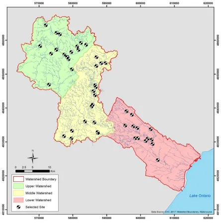
Figure 4.1 – Selected sites within the Credit River watershed. ... 48

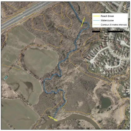
Figure 4.2 – Sinuous low-order channel with degree of regular meandering (Reach LC3). ... 50

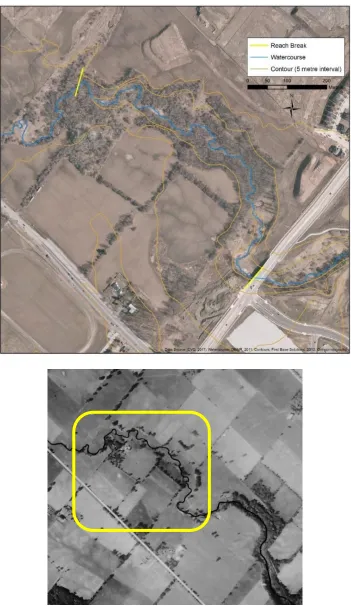
Figure 4.3 – Irregular meandering apparent in a medium-sized watercourse (Reach FC1). ... 51

Figure 4.4 – Larger fluvial system with regular meandering tendencies (Reach CR11). ... 52

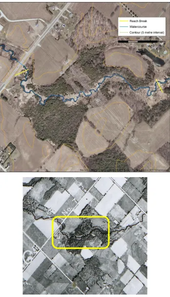
Figure 4.5 – Watercourse which exhibits relative stability from 1954-2013 (Reach HC1). ... 54

Figure 4.6 – Watercourse which exhibits relative stability from 1954-2013 (Reach BC2). ... 55

Figure 4.7 – Watercourse which exhibits relative instability from 1954-2013 (Reach LCR1). ... 57

Figure 4.8 – Watercourse which exhibits relative instability from 1954-2013 (CR9). ... 58

Figure 4.9 – GIS-based drainage area measurement flow chart. ... 60

Figure 4.10 – Reach delineation (Reach BC2). ... 64

Figure 4.11 – Meander axis identification (Reach BC2). ... 65

Figure 4.12 – Meander belt delineation (Reach BC2). ... 67

Figure 5.1 – OLS relation of meander belt width and mean bankfull channel width. ... 79

Figure 5.2 – RMA regression model for meander belt width and mean bankfull channel width. 80 Figure 5.3 – OLS relation of meander belt width and discharge. ... 81

Figure 5.4 – RMA regression model for meander belt width and discharge. ... 82

Figure 5.5 – OLS relation of meander belt width and drainage area. ... 83

Figure 5.6 – RMA regression model for meander belt width and drainage area. ... 84

Figure 5.7 – OLS relation of meander belt width and meander amplitude. ... 85

(8)

vii Figure 5.9 – OLS relation of meander belt width and meander amplitude with the addition of

mean bankfull channel width. ... 86

Figure 5.10 – Discretization of the OLS model for meander belt prediction via mean bankfull channel width using the median of bankfull width at 6.10 m. ... 88

Figure 5.11 – Discretization of the OLS model for meander belt prediction via discharge using the median of discharge at 9.23 m3/s. ... 88

Figure 5.12 – Discretization of the OLS model for meander belt prediction using drainage area, with the median of drainage area at 25.3km2. ... 89

Figure 5.13 – Discretization of meander belt width OLS relation to mean bankfull channel width using watershed zones... 90

Figure 5.14 – Discretization of meander belt width OLS relation to discharge using watershed zones. ... 90

Figure 5.15 – Discretization of meander belt width OLS relation to drainage area using watershed zones. ... 91

Figure 5.17 – Organization of meander belt width and discharge by Strahler stream order. ... 92

Figure 5.18 – Organization of meander belt width and drainage areas by Strahler stream order. 93 Figure 5.19 – OLS relation of discharge and drainage area. ... 95

Figure 5.20 – OLS relation of mean bankfull channel width and discharge. ... 97

Figure 5.21 – OLS relation of mean bankfull channel width and drainage area. ... 97

Figure 6.1 – Meander belt width measurement discrepancies. ... 103

Figure 6.2 – Comparison of OLS meander belt width prediction models using bankfull width. 105 Figure 6.3 – Comparison of OLS meander belt width prediction models using discharge. ... 107

Figure 6.4 – Comparison of OLS meander belt width prediction models using discharge and bankfull width. ... 108

(9)

viii

List of Tables

Table 2.1 – Concepts of river corridor management. ... 4

Table 2.2 – Planimetric Procedures for Meander Belt Delineation. ... 14

Table 2.3 – Empirical Models for Meander Belt Delineation. ... 16

Table 2.4 – Channel type as defined by sinuosity ratio. Source: Charlton, 2008. ... 24

Table 3.1 – Sources and measurement of data used in statistical analysis. ... 43

Table 5.1 – Meander belt width and hydrogeomorphic parameter correlation coefficients. ... 72

Table 5.2 – Correlation matrix for significantly related hydrogeomorphic variables. ... 74

Table 5.3 – Relations of discharge and drainage area in southern Ontario. ... 94

Table 5.4 – Regional models for bankfull channel width via drainage area... 96

Table 5.5 – Relations of meander amplitude and channel width. ... 99

Table 6.1 – Bankfull width models for meander belt width prediction. ... 105

Table 6.2 – Discharge relations for meander belt width prediction. ... 107

(10)

ix

Abbreviations

Abbreviation Property Unit

A Channel cross-sectional area m2

AP Meander amplitude m

D Mean bankfull channel depth m

DA Drainage area km2

MB Meander belt width m

P Sinuosity Ratio

Q2 Discharge m3/s

w Mean bankfull channel width m

S Valley gradient Ratio

ω Total stream power W/m2

(11)

1

Chapter 1 1 Introduction

Policies that restrict land uses and protect stream corridors based on meander belt delineation have

been established in many jurisdictions, including Ontario. The concept of river corridor

management was formulated to address issues surrounding erosion hazards and sensitive habitats.

Rather than viewing a river channel as a liability which requires controls, such as bank hardening

and stabilization, watercourses are now viewed as assets which require space for natural processes

to occur (Piegay H. , Darby, Mosselman, & Surian, 2005). Of the various concepts of river corridor

management and delineation methods that now exist, one of the most commonly used is that of

meander belt delineation.

There are varied definitions of a meander belt, some which restrict the definition to a geometrical

parameter, and some which more broadly define it as the space a watercourse occupies within the

floodplain. The delineation of a meander belt has been identified as a tool for designating a corridor

in which meander migration may occur, with the ultimate goal of limiting development

encroachment, minimizing the loss or damage of property, and protecting natural areas or sensitive

habitats along river systems (Parish Geomorphic, 2004; Kline & Dolan, 2008).

In Ontario, for unconfined watercourses, the Ministry of Natural Resources requires a meander

belt allowance for development restrictions and species-at-risk legislation as part of the

Government of Ontario regulation polices (MNR, 2002). Meander belt delineation is commonly

comprised of planimetric and historical assessments of a watercourse which are used to define an

area of natural meander migration and associated erosional processes. The issue of meander belt

delineation is most prominent for watercourses which have been previously altered and no longer

(12)

2 meander belt delineation is through the application of empirical models that predict meander belt

width from other watershed or channel characteristics. While research concerned with

understanding the mechanics of meandering rivers exists, there is a paucity of research literature

focussing on the hydrologic and geomorphic controls of meander belts. Additionally, upon the

review of river corridor management techniques and meander belt delineation, it is apparent that

there is a lack of consensus on the methods of meander belt measurement to provide basis for these

predictive equations. The applicability and accuracy of models which are frequently used to predict

meander belt width have not yet been assessed for watercourses in southern Ontario.

The purpose of this research project is to evaluate the current standards of practice for meander

belt delineation in southern Ontario, focusing on empirical equations to determine whether these

models can reliably predict belt width. Drawing on a sample population of river reaches in the

Credit River watershed, this research will add to the database of meander belt literature which is

currently limited for watercourses in southern Ontario.

(13)

3

Chapter 2 2 Review of River Corridor Management and Meandering

Channels

2.1 General Principles of River Corridor Management

Perceptions of fluvial governance have shifted in regions of Europe and North America from a

preventative approach (i.e., bank hardening and protection) to a management approach which

focusses on allowing rivers to migrate freely within a delineated space, protecting natural

processes and providing safety for infrastructure; hence, the concept of river corridor management.

The concept of river corridor management has been said to have originated from the increased

awareness of the unsustainable nature and economic cost of engineered bank protections, as well

as the key role of channel dynamics and ecosystem services provided by uninhibited watercourses

(Thorne, Hey, & Newson, 1997; Piegay H. , Darby, Mosselman, & Surian, 2005). Several types

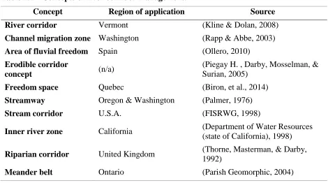
of river corridor management have been developed under a variety of names, as displayed in Table

2.1. The specific definitions and methods of the river corridor concepts vary; however, these

approaches are fundamentally parallel in their purpose of predicting areas at risk of future channel

erosion and associated conservation to help reduce threats to existing infrastructure, human

developments and critical habitats. However, when considering the regions of application for each

of the listed management concepts, it may be inferred that there is a regional association with river

(14)

4

Table 2.1 – Concepts of river corridor management.

Concept Region of application Source

River corridor Vermont (Kline & Dolan, 2008)

Channel migration zone Washington (Rapp & Abbe, 2003)

Area of fluvial freedom Spain (Ollero, 2010)

Erodible corridor

concept (n/a)

(Piegay H. , Darby, Mosselman, & Surian, 2005)

Freedom space Quebec (Biron, et al., 2014)

Streamway Oregon & Washington (Palmer, 1976)

Stream corridor U.S.A. (FISRWG, 1998)

Inner river zone California (Department of Water Resources

(state of California), 1998)

Riparian corridor United Kingdom (Thorne, Masterman, & Darby,

1992)

Meander belt Ontario (Parish Geomorphic, 2004)

2.2 Planimetric and Historical Assessment Methods for River

Corridor Management

The most common approach to delineating a river corridor is through planimetric assessments of

a watercourse (Thorne, Hey, & Newson, 1997; Lagasse, Zevenbergen, Spitz, & Thorne, 2004;

Piegay H. , Darby, Mosselman, & Surian, 2005). Historical data, including topographic maps and

aerial imagery, are used to identify channel geometry variables (e.g., channel sinuosity, meander

wavelength, bankfull channel widths), rates of channel mobility (e.g., rates of erosion and

floodplain turnover rates), and structures preventing channel migration (e.g., bank protection and

infrastructure). Field data, including riparian vegetation, bed and bank substrate, channel

dimensions, fluvial features, and mass movements, are used to supplement the remotely-sensed

data collected on a watercourse. With this information, the historical dynamics of a watercourse

can be assessed in order to predict channel behaviour in the future. Generally, channel mobility is

(15)

5 configurations of the watercourse. The product of this data is used to determine the extent of a

river corridor. Three examples of river corridor delineation methods, which were selected based

on different detailed approaches to river corridor delineation, are described and compared in the

sections to follow.

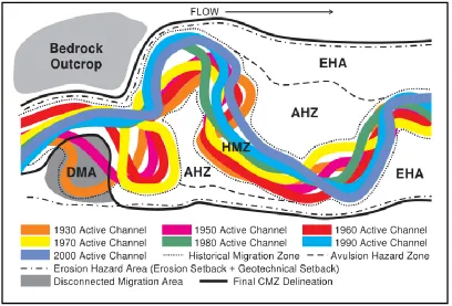
2.2.1 Channel Migration Zone

The concept of a channel migration zone is one example of a river corridor which is delineated

using planimetric assessment for channel which are assumed to be actively meandering; thus,

having associated erosion hazards. To delineate a channel migration zone, four distinct areas must

be identified: the hazard migration zone, avulsion hazard zone, erosion hazard area, and the

disconnected migration area (Rapp & Abbe, 2003). This method requires overlays of previous

channel configurations (Figure 2.1) to identify rates of erosion and directional movement of

meanders, as well as physical characteristics surrounding the watercourse, such as bed

stratigraphy, riparian vegetation, and structures which prevent channel migration. The restricting

characteristic of this methodology is that the channel must be actively migrating to delineate the

(16)

6

Figure 2.1 – Channel migration zone delineation, from Rapp & Abbe (2003).

(HMZ - Historical Migration Zone, AHZ – Avulsion Hazard Zone, EHA – Erosion Hazard Zone, DMA – Disconnected Migration Area)

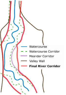
2.2.2 River Corridor (Vermont)

The process of identifying a river corridor, as described by the Vermont Agency of Natural

Resources (Kline & Dolan, 2008), has been automated using the GIS extension, titled Stream

Geomorphic Assessment Tool (SGAT), which identifies the limits of a river corridor in a four-step

process. The corridor is created using the product of a space delineated parallel to the watercourse

centreline (watercourse corridor), a space parallel to the meander centreline (meander corridor),

and a space parallel to the valley wall (Figure 2.2). The GIS extension uses variables such as

bankfull channel width, valley wall position, sinuosity, and centrelines to delineate a final river

(17)

7 approach to delineating a river corridor, however the designated corridor which is output from the

automation tool may be arbitrary and require further analysis for proper corridor delineation.

Figure 2.2 – River corridor delineation, adapted from Kline & Dolan (2008).

2.2.3 Freedom Space

Freedom space is a river corridor concept which integrates flooding as well as the erosion and

migration processes occurring within a fluvial system into the space permitted for natural river

processes to occur (Biron, et al., 2014). The freedom space limits are conceptualized with two

distinct spaces: mobility space and flooding space. To delineate the mobility space, historical rates

(18)

8 extension uses transects across multiple years of channel configurations to generate a quantitative

representation of channel migration. The flooding space is determined by identifying distinctive

landforms suggesting flood processes, and relating them to the severity of flooding (low, medium,

high). Together, the mobility space and flood space are used to delineate three types of freedom

space: minimum (Lmin), functional (Lfunc), and rare (Lrare), based on the likelihood of channel

migration and flooding (Figure 2.3). Expert practitioners can then determine which freedom space

is most necessary for a particular watercourse.

Figure 2.3 – Freedom space delineation, from Biron et al., (2014).

2.3 Limitations of Planimetric and Historical Assessments

There are various limitations associated with the planimetric approach of delineating river

(19)

9 channel features and delineate river corridors. Planimetric analyses are only appropriate if the

channel is sufficiently large to be identified clearly on maps or images, and if channel movement

can be observed from one survey to another (Piegay H. , Darby, Mosselman, & Surian, 2005; Rapp

& Abbe, 2003). This dependency on map or image quality is also largely influenced by the scale

of the mapping medium. Although high resolution data may be acquired for more recent years,

historical imagery is often subject to lower resolutions, making it difficult to accurately map

watercourses. Additionally, the accuracy of the delineated river corridor is dependent on the time

span covered by the obtained mapping materials, which are commonly independent of the temporal

distribution of flooding and migration activity (Piegay H. , Darby, Mosselman, & Surian, 2005).

For migration analyses, this limitation is magnified as high-resolution historical images may be

required for delineation. It has been recommended that historical and current imagery have a scale

of 1:10,000 or 1:20,000 be used in overlay procedures (Thorne, Hey, & Newson, 1997; Parish

Geomorphic, 2004). In some cases, obtaining imagery for current channel configuration may be

difficult due to stream size, vegetation cover, or remote locations. Acquiring the necessary data

for planimetric assessments can be difficult for many watercourses. Moreover, errors associated

with image registration, georeferencing, and feature measurement can be introduced in planimetric

analyses, which can jeopardize the accuracy of river corridor delineation which are based on

historical migration (Rapp & Abbe, 2003).

2.3.1 Summary

The methods of river corridor management discussed above are a few examples of those

approaches grounded in the use of planimetric analysis of historical data (e.g., topographic maps

and aerial photography) and field data to develop an understanding of the watercourse dynamics.

(20)

10 which may be due to the varying locations at which they are applied by prioritizing and

emphasizing certain aspects of river migration, and erosion and flooding hazards. Additionally,

while some of these methods rely on more simplistic map and image overlays to track previous

channel migration, others have adopted more GIS-based or computer-automated programs.

Despite the differences in automated or manual delineation, these methods of river corridor

management have a common goal of outlining the space a watercourse needs for natural river

migration processes to occur, protecting sensitive habitats and mitigating fluvial erosion threats to

infrastructure. Nonetheless, these methods are still confined by limitations: the availability of

historical data, erroneous conclusions introduced by mapping and measurement techniques, the

applicability for altered watercourses, and the repeatability and reliability of the methods when

applied to a specific watercourse.

2.4 Meander Belt as a Method of River Corridor Management

Meander belt is a term which is used to describe the space a meandering watercourse occupies

within the floodplain. The width of a meander belt is of particular interest as it defines the area

that the watercourse occupies or can occupy in the future; thus, providing a quantitative

measurement of a river corridor. Jefferson (1902) first coined the term meander belt as, “the width

of the belt of meanders between lines tangent along the swings of the river.” For many descriptions

of meander belt, this definition is similar. For example, Annable (1996) defines meander belt as

the, “greatest lateral width of the meander pattern within the trend of the valley.” Similarly, Ackers

and Charlton (1970) define meander belt width as the width between parallel lines which contain

the meandering channel. However, there is literature which fails to follow set definition, such as

Carlston (1965), who defines meander belt width as the average width of meanders in a river reach,

(21)

11 discrepancies in meander belt definition, the term is commonly used throughout literature which

focusses on meander geometry and planform.

The Ontario Ministry of Natural Resources’ (MNR) Water Resources Section published the

Technical Guide for River and Stream Systems: Erosion Hazard Limits in 2002. The guide was

prepared, “to provide a consistent standardized procedure for the identification and management

of riverine erosion hazards in the Province of Ontario,” in order to assist in the understanding of

regulations in the 1996 Ontario Provincial Policy statement (MNR, 2002). Within the Provincial

Policy statement, the discussion of meander belt delineation requirements is scarce, simply stating

that development shall be generally directed to areas outside of erosion hazards or the “predicted

meander belt of a watercourse,” (Section 3, Policy 3.1.1) (Ontario Ministry of Municipal Affairs,

1996). This is reiterated in the Conservation Authorities Act: Ontario Regulation 97/04 where it is

stated that a regulation shall prohibit development within the “predicted meander belt of a

watercourse” (Government of Ontario, 1990). Meander belt delineation is also discussed in the

Endangered Species Act (2007) in relation to Redside Dace (Clinostomus elongates), indicating

habitat is considered as, “the area encompassing the meander belt width” (Government of Ontario,

2007). Despite the brief discussion of meander belt delineation in Ontario regulatory documents,

there is still ambiguity in regards to the circumstances in which a meander belt delineation is

unequivocally required.

The most detailed discussion of meander belt delineation is within the MNR (2002) technical guide

for erosion hazard limits. The document states three main components of erosion hazards: natural

processes of erosion, flooding, and slope stability (MNR, 2002). Fluvial systems are classified in

the guide as confined or unconfined. Confined systems are defined as, “ones in which the physical

(22)

12 from the surrounding landscape,” (MNR, 2002). This definition differs from that of the more

specific and standard geomorphology definition in which confined systems are where, “the channel

is bordered on either side by banks that are higher than the highest flood level, or by valley sides,”

(Ashmore & Church, 2001). Unconfined systems are defined as, “ones in which a river or stream

is present but there is no discernible valley slope that can be detected,” (MNR, 2002). Erosion

hazard allowances are varied based on the type of confinement, as seen in Figure 2.4. For

unconfined systems, the guide states a meander belt allowance is necessary. However, in many

cases meander belts are also delineated by practitioners for confined systems.

Figure 2.4 – Erosion hazard allowances by channel confinement, from MNR (2002).

The document defines a meander belt allowance as the maximum extent that a water channel

migrates (MNR, 2002). It is recommended that the meander belt allowance is calculated by 20

(23)

13 protocol is said to be based on available information, yet lacks reference to any supporting data.

The technical guide allows for alternative approaches, in that, “if the proponent determines that

the recommended [procedure] is not appropriate for their location, they must provide […] an

analysis of the meander belt width which can be determined through accepted scientific and

engineering study,” (MNR, 2002). For those locations where other analyses seem required, the

Belt Width Delineation Procedure document, prepared by Parish Geomorphic Ltd. (2004) for the

Toronto and Region Conservation Authority (TRCA), appears to be the preferred alternative.

The TRCA report (Parish Geomorphic, 2004) was created to recommend a protocol for the

delineation of meander belt width for river systems within the TRCA jurisdiction, but is generally

adopted by other Conservation Authorities throughout southern Ontario. The document was

authored by consulting company Parish Geomorphic. The document references an extensive list

of academic literature concerned with meander geometry and morphological assessment.

However, as the report was intended for TRCA use and to provide recommendations within set

jurisdiction, the contents of the document were not subject to a critical or peer-review process.

Nevertheless, the document is used widely across southern Ontario as the primary means of

delineating a meander belt. Here, meander belt is defined as the space a watercourse occupies on

its floodplain in which all natural channel processes occur (Parish Geomorphic, 2004). There are

five core procedures within the report which may be used to delineate a meander belt, of which

four are based on the planimetric assessment of a watercourse (Procedures 1-4). Each of the

procedures follow the same methodology for reach delineation, meander belt axis identification,

and historical analyses (where applicable). The procedures differ based on the current and/or

anticipated state of the watercourse, demonstrated as the scenario in Table 2.1. Procedure 1 was

(24)

14 planning-level studies. Procedures 2-4 were designed for an accurate delineation of a meander

belt, which requires more detailed analysis of historical and current channel configurations, and

anticipated hydrologic scenarios for the watercourse.

Table 2.2 – Planimetric Procedures for Meander Belt Delineation.

Source: Parish Geomorphic (2004).

Procedure Scenario Meander Belt Width Calculation

Procedure 1 Preliminary belt width

delineation

Tangential lines are drawn along extreme meander bends to generate a preliminary belt width (B). Corrections are made based on channel confinement and incision.

Procedure 2 Change in the hydrologic

regime isnot anticipated.

If the existing belt width is < 50m:

Final Belt Width = Belt Width + D + E

If the existing belt width is > 50m:

Final Belt Width = Belt Width * 1.10 + E

Procedure 3

Change in the hydrologic regime is anticipated. (Increase in duration of flows and in frequency of occurrence).

If the existing belt width is < 50m:

Final Belt Width = (Belt Width*1.05) + D + E

If the existing belt width is > 50m:

Final Belt Width = Belt Width * 1.20

Procedure 4

Change in the hydrologic regime is anticipated. (Increase in peak flows and frequency of occurrence).

Final Belt Width = (B + C + D) * adjustment ratio

B = Preliminary Belt Width, C = average bankfull width, D = distance migrated in 100 years (estimated with migration rate), E = distance meander axis shifted in 10-years

2.5 Empirically-Based Models for Corridor Prediction

Knowledge of geomorphic and hydrologic variables which relate to a channel’s ability to migrate

within the landscape has permitted the conception of empirical models which predict meander

(25)

15 relations have been adapted and applied as a tool of estimating and predicting meander belt width

through the collection of empirical data on watercourses where the related hydrologic and

geomorphic variables have been measurable. The models are used primarily as a method of

assessing smaller or low-order watercourses lacking the necessary historical mapping materials

and watercourses which have been altered and may no longer demonstrate a ‘natural’ configuration

(Parish Geomorphic, 2004), as well as a substitute for time-consuming planimetric analyses. Table

2.3 lists several empirical equations which have been developed to estimate meander belt width

(MB) based on other properties of the river channel and/or watershed.

The most common variables used to predict meander belt width are channel and meander geometry

variables, including meander wavelength, radius of curvature, and bankfull channel measurements.

Hydrologic parameters are also employed, including stream power and discharge. However, a brief

review of the empirical models in Table 2.4 demonstrates large discrepancies among coefficients

in equations which relate the same variable to meander belt width. For example, based on these

relations, meander belt width ranges from 4.3 to17.6 times the bankfull channel width. These

inconsistencies may be, in part, due to the spatial variability of watercourses, resulting in

site-specific empirical equations based on the watercourses from which they were developed. From the

empirical equations in Table 2.3, only the models established by Annable (1996) and Parish

Geomorphic (2004) were developed on watercourses from the region of southern Ontario. Annable

(1996) developed his empirical relations from 47 primarily rural watersheds in southern Ontario.

However, he states that the equations display low levels of reliability, as seen by the goodness of

fit statistics, and should only be applied as “…first-order approximations of gross-scale channel

characteristics related to basin scale studies” (Annable, 1996). Therefore, these relations are not

(26)

16

Table 2.3 – Empirical Models for Meander Belt Delineation.

Source Variables Model Reliability Conditions

Ackers &

Charlton (1970) Discharge (Q)

MB = 18.50 Q0.51

MB / w = 2.17 Q0.19

λ / MB = 2.06 Q-0.04

S.E. = 0.21

S.E. = 0.23

S.E. = 0.18

Annable (1996) Bankfull

discharge (Qbf)

MB = 56.95 Qbf0.45

MB = 16.30 Qbf0.88

MB = 131.26 Qbf0.29

S.E. = 0.34

S.E. = 0.29

S.E. = 0.01

Rosgen C – type

Rosgen E – type

Rosgen F – type

Bridge & Mackey (1993)

Hydraulic depth

(DH) MB = 59.90 DH

1.8

Carlston (1965) Mean annual

discharge (Qa) MB = 65.80 Qa

0.47 _r2_{= 0.96}

Collinson (1978) Maximum

depth (Dmax) MB = 65.60 Dmax

1.12

Jefferson (1902) Bankfull width

(w) MB = 17.60 w

Lorenz et al. (1985)

Bankfull width

(w) MB = 7.53 w

1.01 Parish Geomorphic (2004) Total Stream power (ω) Drainage area (DA)

MB = -14.827 +

8.319ln (ω * DA)

r2 = 0.739

S.E. = 8.63

DA < 25 km2

Ward et al. (2002) Bankfull width

(w) – in feet MB = 4.00 w

1.12 Williams (1996) Meander wavelength (λ) Radius of curvature (Rc) Bankfull width (w) Bankfull depth (D)

MB = 0.61 λ

MB = 2.88 Rc

MB = 4.30 w1.12

MB = 148.00 D 1.52

r2 = 0.98

r2= 0.96

r2_{= 0.92}

r2 = 0.81

8 < λ < 23,200 m

2.6 < Rc < 36,000 m

1.5 < w < 4,000 m

0.03 < d < 18 m

(27)

17 For highly modified watercourses, Parish Geomorphic Ltd. derived an empirical equation to

predict expected or potential meander belt width from drainage area and stream power of a

watercourse (Procedure 5). Stream power is a quantitative description of the potential of flowing

water to perform geomorphic work as it moves along an energy gradient (Leopold, Wolman, &

Miller, 1964). Stream power can be defined by the total stream power (ω), the power per unit

length of the channel in watts per square metre, or by specific stream power (Ω), as the power per

unit area of the channel in watts per metre. Stream power has been used as a predictor of channel

dimensions and channel pattern (Magilligan, 1992; Knighton, 1999), and as a predictor of channel

mobility (Bull, 1979; Magilligan, 1992). Therefore, stream power may be a likely control of

meander belt width by controlling migration rates and overall channel dimensions. The TRCA

report (Parish Geomorphic, 2004) does not provide the supporting data (watercourse locations,

river characteristics, statistical methods, etc.) from which the empirical equation was developed.

Additionally, incorporating both stream power and drainage area in the relation appears redundant,

as drainage area is highly correlated with discharge, and therefore, drainage area may be used, “as

a surrogate for discharge in empirical studies of channel morphology” (Knighton, 1999). As stated,

the results from the empirical analysis by Parish Geomorphic (2004) are often compared with other

meander belt width relations, primarily those of Williams (1986). Alternatively, other relations are

employed in lieu of the empirical analysis by Parish Geomorphic, including those of Lorenz et al.

(1985) and Ward (2002).

2.5.1 Limitations of Empirically-Based Models

Empirical equations which relate hydrologic and geomorphic watercourse characteristics offer a

way to estimate and predict meander belt dimensions, reducing the extensive data needs of

(28)

18 exhibit the site-specific nature apparent in planimetric assessments. For instance, Williams (1986)

and Ward et al. (2002) both state the application of their respective equations are feasible for

meander belt width quantification, despite the large discrepancies among coefficients which relate

meander belt width to bankfull channel width. It has been indicated that poor correlations among

meander properties is likely due to the strong control of stream bank erodibility and other local

factors which control meander size (Leopold & Wolman, 1960; Shahjahan, 1970). This suggests

that the relationships developed between meander belt width and channel geometry features may

be unique to the specific watercourses for which they were developed, or conversely, do not

include all relevant variables for meander belt delineation. Although the site-specific nature of

these equations has been acknowledged (Piegay H. , Darby, Mosselman, & Surian, 2005;

Shahjahan, 1970), whether it be the type of stream or geomorphic characteristics of the region,

empirical relations continue to be applied on watercourses outside of the range of stream size or

type for which they were developed.

2.5.2 Summary

Empirical relations offer an opportunity to estimate the size of a river corridor, specifically the

width of a meander belt, when planimetric assessments are not feasible. Several empirical

equations for the estimation of meander belt width exist which employ both hydrologic and

geomorphic variables. Furthermore, empirical relations, such as Williams (1986) and Ward et al.

(2002), have been used as part of meander belt width justification, but their validity has not been

tested for data from southern Ontario rivers, and the relation by Parish Geomorphic (2004) based

(29)

19

2.6 Characterization of Meandering Channels

Meandering channels may be characterized as single-thread channels with sinuous planform which

is comprised of a series of loops or meander bends (Hooke, 2013). They are differentiated from

braided rivers on the continuum of river patterns based on their more stable single-thread

configuration which commonly exhibit higher sinuosity values (Leopold, Wolman, & Miller,

1964; Lagasse, Spitz, Zevenbergen, & Zachmann, 2004; Hooke, 2013). Meandering channels

commonly exhibit an undulating river bed which alternates between deep and shallow sections,

commonly referred to as pool-riffle formations (Leopold, Wolman, & Miller, 1964). This vertical

spatial variation along the length of a channel also influences the lateral planform of the channel

within meandering systems, as pools are commonly associated with meander bends where erosive

forces are concentrated. Figure 2.5 displays the common features of river meanders in an idealized

symmetrical meander bend.

Figure 2.5 – Common features of river meanders, from Hooke (2013).

Unlike the idealized meander shown in Figure 2.5, most meanders appear to be inherently

(30)

20 loops in nature are absolutely identical,” resulting in the inadequacy of the single symmetrical

geometric form to describe all meander loops. Despite this notion and the widespread display of

asymmetrical meandering tendencies, many initial theories of meandering channels assumed

symmetry of meander planform.

Rather than confining the classification of meanders to a simple symmetrical form, a broader range

of more complex meander configurations are now utilized. Brice (1974) suggested meander loops

be assessed as either simple symmetrical loops, simple asymmetrical loops, or compound loops

(Figure 2.6). The evolution of the awareness that meander loops can range in form has also been

applied to meandering patterns at larger scales which incorporate several successive meanders. For

example, compound patterns have also been described as a second meandering tendency

(31)

21

Figure 2.6 – Classification of meander loops, from Brice (1974).

In addition to the irregularity and pattern of a channel, meandering watercourses can be classified

and defined by stability: whether they are actively migrating laterally and downstream, or are more

relatively stable. A classification method of assessing channel stability was developed by Brice

(1975) and further modified by Lagasse et al. (2004); it classifies channels by sinuosity and by

variation in channel width (Figure 2.7). Brice (1982) found that channels which do not vary

significantly in channel width are relatively stable, while channels which are wider at the apex of

(32)

22 assessing channel stability. Combining the width-variability criterion and sinuosity enabled the

formation of a classification system for meandering channels. Nevertheless, the numerous forms

of meander migration and meander patterns may cause difficulty in placing particular reaches

within such classifications.

Figure 2.7 – Meandering channel pattern classification, from Thorne (1997), modified from

(33)

23

2.7 Anatomy of Meander Bends

Meandering channels are often described by their shape, which can be quantitatively measured by

a defined set of geometric parameters. Knowledge of meander geometry allows for the

classification of watercourses, permitting the identification of similarities among meandering

channels and comparisons among states of stability based on meander planform. It has been

suggested that meander geometry of a channel is scaled to that of channel width, dominant

discharge, stream power or drainage area (Thorne, Hey, & Newson, Applied Fluvial

Geomorphology for River Engineering and Management, 1997). This follows similar theories of

hydraulic geometry developed by Leopold and Maddock (1953), where river dimensions are scaled

to discharge or drainage area. This notion offers insight as to which parameters may be most

influential of meandering patterns, and thus, which may be most pertinent in meander belt width

estimation.

Meander geometry has been reduced to a manageable number of parameters. Ferguson (1975)

suggested a three-component pattern continuum framework, in which meandering rivers are

characterized by three planimetric properties: the complexity of meandering, the scale of

meandering, and the degree of irregularity. Parameters that are commonly used to address this

include sinuosity (complexity), meander wavelength (scale), meander amplitude (scale), and

radius of curvature of a bend (scale and irregularity) (Figure 2.8). Details of these parameters are

(34)

24

Figure 2.8 – Definition of key meander geometry parameters.

2.7.1 Sinuosity

The sinuosity of a channel has been defined as a measure of the degree of complexity or

curvilinearity displayed within a meandering channel (Andrle, 1996). Sinuosity (P) is commonly

measured as a ratio between the length along a channel (LC) to the length of the valley (LV) within

a given reach (Figure 2.8). Ratios are frequently compared to a sinuosity index (Table 2.4). The

threshold values of the sinuosity index are widely used; however, are arbitrary in nature, as the

values are not based on physical differences related to meandering (Charlton, 2008).

Table 2.4 – Channel type as defined by sinuosity ratio. Source: Charlton, 2008.

Sinuosity Ratio Channel Type

<1.1 Straight

1.1-1.5 Sinuous

>1.5 Meandering

For a given sinuosity value, there are numerous channel configurations which are possible (Figure

(35)

25 confirmed by Hooke & Yorke (2010), who found a relatively constant sinuosity value in a

meandering reach despite observing major changes in the shape and length of individual meander

bends. Sinuosity is greatly influenced by the scale at which channel parameters are measured.

Figure 2.9 – Configurations for sinuosity index of 1.5, from Hey (1976).

Mueller (1968) and Ferguson (1975) proposed hydraulic and topographic sinuosity indexes to

account for physical attributes of a watercourse, which incorporates a measurement described as

the “air” distance, or shortest distance from the source to the mouth of a watercourse. Additionally,

a surrogate of sinuosity was developed by Andrle (1996) in a method titled the angle measurement

technique, where a characteristic angle (Ac) defines the maximum degree of complexity. Although

this variable is not synonymous with sinuosity, it provides a measure of the scale of complexity

while eliminating the scale-dependent nature of sinuosity measurements. Nevertheless, the

traditional measurement of sinuosity continues to be employed for the purpose of classifying the

scale of complexity apparent in meandering channels.

2.7.2 Meander Wavelength

Meander wavelength (λ) has been defined as a measure of the scale of meandering within a channel

by quantifying the spacing of successive meander bends (Leopold & Wolman, 1960; Andrle, 1996;

(36)

26 of the downstream scale of meandering, rather than a lateral migration measurement. Meander

wavelength is determined by doubling the straight-line distance between two successive points of

inflection (Figure 2.8). However, this measurement is complicated by irregularities in channel

pattern. Ambiguity can be introduced when defining points of inflection, particularly in small

channels or when irregularities are apparent. Another issue apparent with meander wavelength

measurements is the selection of an “average” pair of meanders for assessment which can result in

the misrepresentation of a channel (Ferguson, 1975). A detailed characterization of meander

wavelengths is that of spectral analysis where a dominant wavelength may be identified (Speight,

1965; Chang & Toebes, 1970; Ferguson, 1975).

There is a well-established relationship between meander wavelength and channel width, dating

back to work by Leopold and Wolman (1960), which has allowed for the derivation of empirical

equations to estimate meander wavelength. It can be said that meander wavelength bears a

relatively constant ratio with channel width, ranging from approximately six to twelve times

channel width. Although these equations suggest identifiable underlying tendencies in meander

morphology and channel dimensions, they are only approximations of true relations (Williams,

1986). Therefore, care must be taken in applying and relying on such empirical relations to

quantify the scale of meandering in a channel.

2.7.3 Meander Amplitude

Meander amplitude is a measure of the lateral extent of a meander (Figure 2.8), defined as the

lateral distance between tangential lines drawn to the centre of a channel across two successive

meander bends (Leopold, Wolman, & Miller, 1964). As meander amplitude is measured on a set

of meander bends, in order to describe a channel at a reach scale, a governing meander amplitude

(37)

27 meander amplitude measurements; however, it has been shown to poorly correlate with other

meander geometry or channel characteristic variables (Leopold, Wolman, & Miller, 1964;

Williams, 1986). It has been inferred that meander amplitude may be controlled more by local

characteristics of the channel, such as the stability of the banks and erosive forces occurring within

the watercourse, rather than any hydrogeomorphic principles (Leopold, Wolman, & Miller, 1964).

2.7.4 Radius of Curvature

Radius of curvature (Rc) can be determined by fitting a circle to the centre line or outer bank of

the meander bend and measuring the radius of the inscribed circle (Figure 2.8). Similar to meander

amplitude, radius of curvature is a parameter which is not measured at the reach scale, as are

meander wavelength and sinuosity. Brice (1974) inscribed circular arcs on idealized meander loops

to indicate the general geometry and symmetry of meanders which assists in understanding and

classifying meander shape and evolution. This visual assessment of curve fitting has been

enhanced quantitatively by introducing the measurement of radius of curvature of an individual

meander bend. This parameter indicates the tightness of an individual meander, and has been

employed to represent the state of meander regularity and stability (Geist, 2005; Lagasse, Spitz,

Zevenbergen, & Zachmann, 2004). For example, it has been suggested that meanders with larger

radius of curvature measurements display greater stability (Hickin & Nanson, 1984; Geist, 2005).

The process of fitting a single circle to a simple symmetrical or asymmetrical meander bend can

be a relatively straightforward task. However, fitting single circles to complex or compound bends

can be difficult and more subjective.

2.7.5 Limitations of Meander Geometry Measurement

Despite the various benefits, there are significant limitations to measuring meander geometry.

(38)

28 maps and aerial photographs as a medium of measurement, as well as the subjectivity of

delineating meander parameters.

Although the introduction of aerial photography has reduced many of the errors associated with

topographic maps, issues concerning distortion and scale remain. The scale at which aerial

photography is taken greatly affects the accuracy of meander geometry quantification, especially

with small watercourses displaying complex and minor meander configurations. Enhancing

photographs, specifically those which are historical, can result in the distortion of a channel. The

accuracy at which meander geometry is delineated is dependent on the scale and quality of the

aerial photographs used; thus, errors will propagate through meander geometry quantification

(Ferguson, 1975).

The measurement of geometric meander variables has been proven to be highly subjective.

Meander sinuosity is largely dependent on the scale of measurement, and the estimation of the

channel and valley lengths can become increasingly difficult with small and complex systems

(Andrle, 1996). The precise measurement of meander wavelength is often difficult and subjective,

due to scaling issues, channel complexity, and the identification of inflection points (Andrle, 1996;

Carlston, 1965; Hooke, 1984). As well as being dependent on the scale of the mapping medium,

radius of curvature measurements are significantly influenced by the method of fitting a circle or

arc to a meander bend (Lagasse, Spitz, Zevenbergen, & Zachmann, 2004).

Finally, the use of meander geometry to predict meander migration is subject to the assumption of

continuity of change (Lawler, 1993). The movement of a meander is assumed to be simple,

continuous, and linearly migrating, which fails to account for the sometimes stochastic and

(39)

29

2.8 Study Rationale and the Case of the Credit River

Current land use management policies and procedures require the application of site-specific

planimetric assessments, or empirical equations, to measure or predict river corridor and meander

belt dimensions. In the case of small, low-order, or highly modified watercourses, the measurement

of meander belt width is driven by the application of empirical relations. However, there is limited

documentation regarding the range of meander morphology in the watersheds of southern Ontario,

and the principle parameters that control meander belt width have not yet been systematically

investigated. Upon analysis of river corridor management techniques and meander belt delineation,

it is evident that there is a lack of knowledge and agreement regarding the methods of meander

belt delineation, and the controls of meander belt development. Therefore, based on the

conclusions of this analysis, the present research aims to shed light on the array of meander

morphology within southern Ontario, incorporating empirical data from a selection of

watercourses within the region, and to develop an empirical relation for meander belt width

prediction and quantification that is both developed for and supported by regionally derived data.

2.9 Research Objectives

The fundamental question driving this investigation is:

What geomorphic and hydrologic variables primarily control meander belt width?

It is anticipated that meander belt width will scale to hydrogeomorphic variables in a similar

manner to other meander geometry parameters. In order to assess the presented research question,

the project has three primary objectives:

1. Document meander morphology and meander belt width over a range of channel sizes and

(40)

30 2. Correlate interactions between meander belt width and primary independent variables:

stream power, drainage area, discharge, bankfull channel dimensions, and channel

configuration.

3. Compare statistical relations of meander belt width prediction developed using the present

data set with previously established relations that are currently used in practice in southern

(41)

31

Chapter 3 3 Data Sources and the Credit River Watershed

3.1 The Credit River Watershed

The Credit River is a tributary to Lake Ontario with a drainage area of approximately 860km2 extending northwest to Orangeville, located on the northern shore of Lake Ontario. The watershed

has a well documented geomorphological database consisting of channel characteristics and

measurements, collected by the Credit Valley Conservation Authority (CVC), which has been

made available for the present research. The availability of data made this research feasible within

the restricted time limits. The watershed displays landscape diversity, covering several distinct

geological settings, many of which are characteristic to southern Ontario. By selecting 46 sites in

a fluvial system that includes representative geomorphic and geological settings and range of river

types and sizes, the study results will be transferrable to similar landscapes in other watersheds in

southern Ontario. The purpose of this chapter is to introduce the Credit River watershed and data

sources used in analysis.

The Credit River was selected for two major reasons:

1. Data availability

2. Landscape diversity

3.1.1 Location

The Credit River is located on the northern shore of Lake Ontario and is part of the Great Lakes

Basin which drains into the St. Lawrence River. The watershed falls under the Credit Valley

Conservation Authority’s (CVC) jurisdiction. The watershed, divided into 23 sub-watersheds,

stretches from its headwaters in Orangeville, Erin and Mono, through nine municipalities,

(42)

32 Ontario, the upstream drainage is 860km2 (Kennedy & Wilson, 2009), with minimum and maximum elevations of approximately 70 and 525 metres above sea level, respectively, giving a

total relief of approximately 455 metres (Figure 3.2).

(43)

33

Figure 3.2 – Credit River Watershed elevation.

3.1.2 Physiography

The Credit River watershed can be divided into three distinct physiographic regions, termed by

the CVC (2009) as the upper, middle, and lower watershed zones (Figure 3.3). The upper

watershed zone, covering 330km2 of the entire catchment, can be characterized by hilly areas of

till plains, moraines, drumlins, and glacial spillways (Figure 3.4). Tributaries located here are

(44)

34 (Kennedy & Wilson, 2009). The river exits the plateau through knickpoints in the Niagara

Escarpment at Cataract and Belfountain, with the main and west branches uniting at the Forks of

the Credit. The middle watershed, approximately 300km2, is comprised of portions of the Niagara

Escarpment, dominated by rock outcrops of dolomitic limestone and shale, and steep terrain. The

Oak Ridges Moraine is a prominent feature in the eastern section of the region. The Credit River

has built a wide alluvial plain on the Lake Ontario plain downstream of the escarpment, the lower

watershed, which is approximately 230km2_{of the catchment (Kennedy & Wilson, 2009). This}

relatively flat topographical area, where the valley is cut into till and underlying shale, leads a

(45)

35

(46)

36

Figure 3.4 – Credit River Watershed physiography.

3.1.3 Hydrology

The Water Survey of Canada operates a total of nine stream-gauges within the Credit River

catchment, of which four stream-gauges on the main branch will be addressed in this thesis. From

upstream to downstream, the gauges are: 02HB013, “Credit River near Orangeville”; 02HB001,

“Credit River near Cataract”; 02HB018, “Credit River at Boston Mills”; 02HB025, “Credit River

at Norval” (Figure 3.5). The gauges have been operational since 1967, 1915, 1982 and 1988,

(47)

37 hydrographs for each gauged station using the historical datasets obtained from Water Survey

Canada. A compilation of annual hydrographs from each of the gauges (Figure 3.10) demonstrates

very little change in discharge since the time the gauges were installed, with the Norval gauge

showing a slight trend with a very low r2value. The lack of a trend suggests that using a discharge

for a particular time period will not greatly impact the results of model development, for this data

set. The hydrographs appear typical for southern Ontario watercourses, and demonstrate little

(48)

38

Figure 3.5 – Water Survey of Canada gauge station locations.

(49)

39

Figure 3.6 – Credit River discharge at Orangeville (1967-2015).

Figure 3.7 – Credit River discharge at Cataract (1915-2015).

0 0.5 1 1.5 2 2.5 3

0 50 100 150 200 250 300 350

Me an Da ily Dis ch ar ge (m 3/s )

Time (Day of the year)

Mean Daily Discharge Median Daily Discharge 90th Percentile 10th Percentile

0 2 4 6 8 10 12 14 16

0 50 100 150 200 250 300 350

(50)

40

Figure 3.8 – Credit River discharge at Boston Mills (1982-2015).

Figure 3.9 – Credit River discharge at Norval (1988-2015).

0 5 10 15 20 25 30

0 50 100 150 200 250 300 350

Mean Daily Discharge Median Daily Discharge 90th Percentile 10th Percentile

0 5 10 15 20 25 30 35 40 45

0 50 100 150 200 250 300 350

(51)

40

Figure 3.10 – Mean annual discharge for Credit River at four main-branch gauge stations.

3.1.4 Land Use

Land use within the Credit River watershed is primarily agricultural and developed land, which

together cover approximately 70% of the basin (CVC, 2009). The lower watershed is heavily

developed, covering the majority of Mississauga and western Brampton (Figure 3.11).

Approximately 80% of the 750,000 living within the Credit River watershed are located within the

lower watershed zone (CVC, 2009). The upper and middle watersheds have remained primarily

agricultural and forested. This is, in part, due to the demand for rural estate properties, with 20%

of agriculture declared as equestrian farms (CVC, 2009), and due to the Greenbelt Legislation

which now protects areas of the Oak Ridges Moraine, Niagara Escarpment, and selected

countryside (Figure 3.12) (Kennedy & Wilson, 2009).

Q = 0.05x - 96.87

r² = 0.06

Q = 0.003x - 0.53

r² = 0.00

Q = 0.001x - 1.81

r² = 0.02

Q = 0.002x - 2.86

r² = 0.03

0 1 2 3 4 5 6 7 8 9 10

1900 1920 1940 1960 1980 2000 2020

(52)

41

(53)

42

Figure 3.12 - Greenbelt boundaries within the Credit River Watershed.

3.2 Data Sources for Analysis

A large amount of data has been collected within the Credit River watershed by CVC in order to

fulfill the Integrated Watershed Monitoring Program (IWMP), which originated in 1999. These

data are of value with respect to the objectives of this thesis, and can be used to determine, analyze,

and validate the findings of meander belt dimensions for the development of a predictive meander

Meander belt delineation: Developing a predictive model for meander belt width

Scholarship@Western

Scholarship@Western

Meander belt delineation: Developing a predictive model for

Meander belt delineation: Developing a predictive model for

meander belt width

meander belt width

Abstract

Keywords

Acknowledgements

Table of Contents

List of Figures

List of Tables

Abbreviations

Chapter 1

1 Introduction

Chapter 2

2 Review of River Corridor Management and Meandering

Channels

2.1 General Principles of River Corridor Management

2.2 Planimetric and Historical Assessment Methods for River

Corridor Management

2.2.1 Channel Migration Zone

2.2.2 River Corridor (Vermont)

2.2.3 Freedom Space

2.3 Limitations of Planimetric and Historical Assessments

2.3.1 Summary

2.4 Meander Belt as a Method of River Corridor Management

2.5 Empirically-Based Models for Corridor Prediction

2.5.1 Limitations of Empirically-Based Models

2.5.2 Summary

2.6 Characterization of Meandering Channels

2.7 Anatomy of Meander Bends

2.7.1 Sinuosity

2.7.2 Meander Wavelength

2.7.3 Meander Amplitude

2.7.4 Radius of Curvature

2.7.5 Limitations of Meander Geometry Measurement

2.8 Study Rationale and the Case of the Credit River

2.9 Research Objectives

Chapter 3

3 Data Sources and the Credit River Watershed

3.1 The Credit River Watershed

3.1.1 Location

3.1.2 Physiography

3.1.3 Hydrology

3.1.4 Land Use

3.2 Data Sources for Analysis