A multiscale method for computing effective parameters of composite electromagnetic materials with memory effects

A MULTISCALE METHOD FOR COMPUTING EFFECTIVE PARAMETERS OF COMPOSITE ELECTROMAGNETIC MATERIALS WITH MEMORY EFFECTS

V. A. BOKIL ∗, H. T. BANKS †, D. CIORANESCU ‡, AND G. GRISO §

Abstract. We consider the problem of computing (macroscopic) effective properties of composite materials that are mixtures of complex dispersive dielectrics described by polarization and magnetization laws. We assume that the micro-structure of the composite material is described by spatially periodic and deterministic parameters. Mathematically, the problem is to homogenize Maxwell’s equations along with constitutive laws that describe the material response of the micro-structure comprising the mixture, to obtain an equivalent effective model for the composite material with constant effective parameters. The novel contribution of this paper is the homogenization of a hybrid model consisting of the Maxwell partial differential equations along with ordinary (auxiliary) differential equations modeling the evolution of the polarization and magnetization, as a model for the complex dielectric material. This is in contrast to our previous work [3] in which we employed a convolution in time of a susceptibility kernel with the electric field to model the delayed polarization effects in the dispersive material. In this paper, we describe the auxiliary differential equation approach to modeling material responses in the composite material and use the periodic unfolding method to construct a homogenized model.

Key words. Maxwell’s equations, Periodic unfolding, Homogenization, dispersive media, auxiliary differential equation.

1. Introduction. Computational simulations of the propagation and scattering of transient electromagnetic (EM) waves in complex materials are important for constructing prediction tools that are reliable [28]. Examples are applications involving radar, environmental and medical imag-ing, such as the noninvasive detection of degradation in materials, the detection of cancerous tumors [16], the investigation of the effect of precursors on the human body, and the design of engineered composites such as ceramic matrix composites (CMC’s) and meta-materials [34]. Thus, the develop-ment and analysis of efficient forward numerical methods which are accurate, consistent and stable has been and continues to be an important area of research in computational electromagnetics.

For some time there has been interest in the integration of silicon nitride carbon based ceramic matrix composites (CMCs) for their use in high temperature turbine engines [2, 24]. As these materials are being investigated for their use in these applications, there is also a need to non-destructively monitor the material’s degradation. In recent efforts [5, 6, 7], the authors were specifically interested in a silicon nitride carbon based CMC. This SiC/SiCN CMC has a silicon carbon fiber and a silicon nitride carbon matrix. Exposure to high temperature environments induces oxidation in the CMC, producing SiO2 and SiN. As discussed in [5, 6, 7, 13, 14], multiple

Lorentz polarization laws (based on the Lorentz model for polarization (6.3) which results from the displacement of electrons from equilibrium under the effect of an interrogating electromagnetic field) are appropriate to use in describing these components.

More recently, there has been increased activity in the design and development of new materials called meta-materials, with tailored EM properties. These materials are a broad class of micro-or nano-structures made up of tailmicro-ored building blocks that are smaller than the wavelength of the interrogating electromagnetic field, thus enabling dense packing into an effective material [33]. Meta-materials are fabricated through engineering design as building blocks for devices with unique

∗

Department of Mathematics, Oregon State University, Corvallis, OR 97331 U.S.A. [email protected].

†

CRSC, North Carolina State University, Raleigh, N.C. 27695-8205, [email protected]. ‡

Universit´e Pierre et Marie Curie, Laboratoire Jacques-Louis Lions, 4, Place Jussieu, 75252 Paris, Cedex 05, [email protected].

§

Universit´e Pierre et Marie Curie, Laboratoire Jacques-Louis Lions, 4, Place Jussieu, 75252 Paris, Cedex 05, [email protected].

EM responses, from the microwave to the optical frequency range [34].

For a complex dispersive dielectric that exhibits a heterogeneous micro-structure described by spatially periodic parameters, we consider an electromagnetic interrogation technique for identi-fying the response of this composite material by subjecting it to electromagnetic fields generated by currents of varying frequencies. When the period of the structure is small compared to the wavelength of the interrogating field, the coefficients in Maxwell’s equations oscillate rapidly, and are difficult to treat numerically in simulations. We use the mathematical theory of homogeniza-tion to produce an equivalent model for efficient simulahomogeniza-tion of the response of the heterogeneous material to the interrogating electromagnetic field. Homogenization is a mathematical method in which a model for a composite material involving spatially dependent parameters (depending on the microscopic structure) is replaced with a model for an equivalent material with macroscopic, homogeneous properties. The limiting homogeneous model with effective constant coefficients is easier to numerically discretize. The approach to homogenization that we take here is based on the periodic unfolding method presented in [11].

For the computation of effective parameters of composite materials, traditional mixture formulas based on physical arguments [29] are available in the literature. Some of the most popular mixing formulas are the Maxwell Garnett formula, the B¨ottcher mixture rule or Bruggeman formula, and the coherent potential formula. The mathematical theory of homogenization has also been applied to Maxwell’s equations in composite materials. In [1, 15, 19, 20, 23, 31, 32, 35] using a variety of techniques, including two scale convergence, homogenized models for Maxwell’s equations in composite materials having anisotropy and memory effects are constructed. In [22], a singular limit approximation of the constitutive laws for chiral media in the time domain are studied, while in [25], an asymptotic homogenization approach for 3D periodic lattices of complex media inclusions with bianisotropic properties is constructed. Additional constructions can be found in [26, 27]. In [9, 36, 37] multiscale numerical methods based on finite elements and finite differences are constructed for the time-dependent Maxwell’s equations with memory effects in composite materials (linear dispersive dielectrics). Numerical homogenization using the heterogeneous multiscale method, and based on two scale convergence for Maxwell’s equations is presented in [10].

In this paper, we use the periodic unfolding method, discussed in detail in [11] in the abstract framework of stationary elliptic equations, to homogenize the time dependent Maxwell’s equations in complex materials that are described by constitutive laws involving the time evolution of the electric polarization and magnetization. We continue our efforts from [3, 8] in which we considered composite materials described by convolutions in time of a susceptibility kernel with the electric and/or magnetic field. The periodicity of the composite material results in spatially periodic pa-rameters in the convolution description of the polarization and magnetization, as well as in the electric permittivity, magnetic permeability and conductivity of the material. In this paper, we use a different but equivalent approach called the auxiliary differential equation(ADE) approach, in which the time evolution of the polarization is modeled by a system of first order ordinary differential equations (ODEs) forced by the electric field. Using an analogous approach for the magnetization, we also include systems of ODEs for the time evolution of the magnetization depen-dent on the magnetic field. Appending these ODEs to the Maxwell partial differential equations (PDEs) gives a hybrid PDE-ODE model for the composite material with spatially varying (pe-riodic) parameters and fields. The homogenization of this hybrid PDE-ODE model provides an alternative homogenized model to the convolution approach in [3, 8] for computing the effective response of the complex composites considered here.

method and the theory developed in [8], we develop the homogenized limit model for Maxwell’s equations considered in this paper. In Section 6, we consider some specific models for linear dispersive and meta materials, and in Section 7, we use the general theory developed in Section 5, to develop the limit homogenized model for a composite material described by the Debye model for orientational polarization with spatially periodic parameters.

2. Maxwell’s equations in a Complex Dielectric. We start with Maxwell’s equations for a linear and isotropic dielectric that includes terms for the electric polarization and magnetization. Consider a timeT >0 and let Ω⊂_R3_{be a bounded domain with Lipschitz boundary∂Ω. Maxwell’s}

curl equations are given as:

∂D

∂t =∇×H−JE in (0, T)×Ω, (2.1)

∂B

∂t =−∇×E−JH in (0, T)×Ω, (2.2)

along with zero Gauss divergence laws

∇ ·D= 0, ∇ ·B= 0 in (0, T)×Ω, (2.3)

in a region Ω with no free charges. The vector valued functions E and H represent the strengths

of the electric and magnetic fields, respectively, while D and B are the electric and magnetic flux

densities, respectively. The external electric and magnetic source current densities are given byJE,

and JH, respectively.

We assume perfect conducting boundary conditions on the boundary ∂Ω given by

n×E= 0 on [0, T]×∂Ω, (2.4)

wheren is the unit normal vector to ∂Ω. We have the initial conditions

E(0,x) =E0, H(0,x) =H0 in Ω. (2.5)

The fields E0,H0 are the initial electric and magnetic fields. We assume that these initial fields

satisfy the Gauss divergence laws.

System (2.1) is completed by constitutive laws that embody the behavior of the material in response to the electromagnetic fields. These are given in the form

D(t,x) =0r(x)E(t,x) +PR(t,x) in (0, T)×Ω, (2.6) B(t,x) =µ0µr(x)H(t,x) +MR(t,x), in (0, T)×Ω. (2.7)

To describe the behavior of the media’s macroscopic retarded (or delayed) electric polarization

PR, and magnetizationMR, we employ a general integral equation model in which the polarization,

and magnetization, explicitly depend on the past history of the electric, and magnetic fields, respec-tively. We assume that there are no free electric charges unaccounted for in the electric polarization

P. The model for polarization is sufficiently general to include microscopic polarization mechanisms

such as dipole or orientational polarization [18] as well as ionic and electronic polarization [17] and other frequency dependent polarization mechanisms leading to linear models [4]. In addition, with nonzero magnetization we can also include the case of the Drude and Lorentz meta material models

[21]. The resulting constitutive laws for the polarization and magnetization can be given in terms of an electric susceptibility kernelνE_{, and magnetic susceptibility kernelν}H _{in the form}

PR(t,x) =

Z t

0

νE(t−s,x)E(s,x) ds, (2.8)

MR(t,x) =

Z t

0

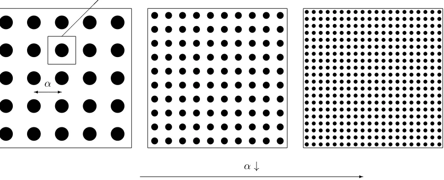
νH(t−s,x)H(s,x) ds. (2.9) 3. The Auxiliary Differential Equation (ADE) Technique: ODE Models for Po-larization and Magnetization. We consider composite materials (see Figure 3.1) which have a periodic micro-structure,α in which the inclusions inside the host matrix, and the host matrix are both described as materials with responses governed by (2.8) and (2.9) . Thus, the polarization, and magnetization vectors PR, and MR are modeled by different susceptibility kernels, one inside

the inclusion and another within the host material. We will consider the case where the

polar-} } } } } } }

Yα Cell

} } } } } } } } } } } } } } } } } } α -v v v v v v v v v v v v v v v v v v v v v v v v v v v v v v v v v v v v v v v v v v v v v v v v v v v v v v v v v v v v v v v v v v v v v v v v v v v v v v v v v v v v v v v v v v v v v v v v v v v v s s s s s s s s s s s s s s s s s s s s

s s s s s s s s s s s s s s s s s s s ss s s s s s s s s s s s s s s s s s s s s s s s s s s s s s s s s s s s s s s s s s s s s s s s s s s s s s s s s s s s s s s s s s s s s s s s s s s s s s s s s s s s s s s s s s s s s s s s s s s s s s s s s s s s s s s s s s s s s s s s s s s s s s s s s s s s s s s s s s s s s s s s s s s s s s s s s s s s s s s s s s s s s s s s s s s s s s s s s s s s s s s s s s s s s s s s s s s s s s s s s s s s s s s s s s s s s s s s s s s s s s s s s s s s s s s s s s s s s s s s s s s s s s s s s s s s s s s s s s s s s s s s s s s s s s s s s s s s s s s s s s s s s s s s s s s s s s s s s s s s s s s s s s s s s s s s s s s s s s s s s s s s s s s s s s s s s s s s s s s s s s s s s s s s s s s s s s s s s s s s s α↓

-Fig. 3.1. A two dimensional periodic composite material presenting a circular microstructure with periodicityα.

The figure showsαdecreasing from left to right. The picture also depicts the cellYα

ization, and magnetization vectors, PR and MR modeled by convolutions of susceptibility kernels

with the electric field E, and magnetic field H, respectively, can be equivalently described by laws

in which the dynamic evolution of PRand MR is given in the time domain, bynth order ordinary

differential equations (ODEs) in the form

NE

X

j=0

aE_j(x)∂

j PR

∂tj (t,x) +β E

0 (x)E(t,x) = 0, (3.1)

NH

X

j=0

aH_j (x)∂

j MR

∂tj (t,x) +β H

0 (x)H(t,x) = 0, (3.2)

on (0, T)×Ω with aE_N

E(x) and a H

NH(x) strictly positive functions of x on Ω. Thus, in the most

discussion on the class of polarization and magnetization laws given by susceptibility kernals that can be equivalently defined using systems of ODEs.

In this paper, we will assume that the host matrix and inclusions are modeled by the same system of ODEs, with the material coefficients aE_i , i = 0, . . . , NE, andaHi , i= 0, . . . , NH, given as

functions of the spatial variablexto accommodate treatment of composite materials and structures. The ODE models for PR and MR can be written as a system of first order ordinary differential

equations. If NE =NH = 1, then this will already be the case. Thus, if NE ≥2 and NH ≥2, we

can rewrite the models as systems of ODEs. To do this, we defineP(0) =PR and M(0)=MR, and

define the time derivatives

P(`+1)= ∂ `

PR ∂t` , M

(j+1) ₌ ∂jMR

∂tj , (3.3)

for`= 0,1, . . . , NE−2 andj= 0,1, . . . , NH−2. Next, for (t,x)∈[0, T]×Ω, we define the vector

functions

P(t,x) =

P(0)(t,x),P(1)(t,x), . . . ,P(NE−1)(t,x)

T

, (3.4)

M(t,x) =

M(0)(t,x),M(1)(t,x), . . . ,M(NH−1)(t,x)

T

. (3.5)

Using (3.4) and (3.5) we can rewrite (3.1) and (3.2) as

(S₁E(x)⊗I3) ∂P

∂t + (S E

2(x)⊗I3)P+ (S3E(x)⊗I3)E=0, (3.6)

(S₁H(x)⊗I3) ∂M

∂t + (S H

2 (x)⊗I3)M+ (S3H(x)⊗I3)H=0. (3.7)

The form of the matrices in (3.6) and (3.7) depend on the values of NE and NH. Case: NE =NH = 1

If the evolution of P and M are governed by first order ODEs, then, for V ∈ {E, H}, i.e., V =E

orV =H, the matrices in (3.6) and (3.7) are of order 1×1, i.e. scalar functions given as

S₁V(x) =aV₁(x), (3.8a)

S₂V(x) =aV₀(x), (3.8b)

S₃V(x) =β₀V(x). (3.8c)

Case: NE ≥2, NH ≥2

Let n, k ∈ _N. We define In to be the n×n identity matrix, and 0n×k to be the n×k matrix of

zeros. We denote0n=0n×n.

In this case, S₁V(x) is a NV ×NV diagonal matrix, with

S₁V(x) = "

INV−1 0 0NV−1 aVNV(x)

#

. (3.9)

The matrixS₂V(x) is theNV×NV matrix with -1 on the super-diagonal, (a0(x), a1(x), . . . , aNV−1(x),0)

in theNVth row and zeros elsewhere. The matrixS₃V(x) is aNV ×1 matrix, with zeros in all rows except the NVth element which isβV0(x).

3.1. Maxwell’s Equations with Polarization and Magnetization Laws. Define n = 3(2 +NE+NH). We define the vector functionu: (0, T)×Ω→Rn given as

u(t,x) = (u1,u2,u3,u4)T = (E(t,x),P(t,x),H(t,x),M(t,x))T. (3.10)

We can rewrite Maxwell’s equations along with the constitutive laws (3.1) and (3.2) in the form

              

(i) A(x)∂u

∂t(t,x) +B(x)u(t,x) =Fu(t,x)−Js(t,x) in (0, T)×Ω,

(ii) u(0,x) =u0 in Ω,

(iii) u1(t,x)×n(x) =0on (0, T)×∂Ω.

(3.11)

In the above, Aand B aren×ndiagonal matrices with the following forms:

A(x) = 

      

0r(x) 01×NE 0 01×NH 0NE×1 S1E(x) 0NE×1 0NE×NH

0 01×NE µ0µr(x) 01×NH 0NH×1 0NH×NE 0NH×1 SH1 (x)



      

⊗I3, (3.12)

while the matrixB is the n×n matrix given by

B(x) = 

     

S₅E(x) S₄E(x) 0 01×NH S₃E(x) SE₂(x) 0N_E×1 0NE×NH

0 01×NE S5H(x) S4H(x) 0NH×1 0NH×NE S3H(x) S2H(x)



     

⊗I3. (3.13)

Case: NE =NH = 1

In this case n = 12. The matrices S_jV(x) for j = 1,2,3 and V ∈ {E, H} are given in Section 3. The additional matrices SV₄(x) andS₅V(x) are scalars defined as;

S₅E(x) =−β E 0 (x) aE₁(x), S

E

4 (x) =− aE₀(x)

aE₁(x), (3.14)

S₅H(x) =−β H 0 (x) aH₁ (x), S

H

4 (x) =− aH₀ (x)

aH₁ (x). (3.15)

Case: NE ≥2, NH ≥2

In this case, matrices S₄E and S₄H are of order 1×NE and 1×NH, respectively, each with a 1 in

the second column and zeros elsewhere. AlsoSE

5(x) = 0 andS5H(x) = 0 are both scalar quantities.

Next, we define the formal (extended) Maxwell operator Mby

Fu(t,x) = ((∇×H)(t,x),03NE×1,−(∇×E)(t,x),03NH×1)T, (3.16)

and the vectorJs as

4. A Priori Estimates. We consider the space

V(Ω) =H0(curl,Ω)×(H(curl,Ω))NE ×H(curl,Ω)×(H(curl,Ω))NH, (4.1) where we define

H(curl,Ω) ={v∈L2(Ω;R3); curlv∈L2(Ω;R3)},

equipped with the norm||v||2 _=|v|2_+|curlv|2_{, and}

H0(curl,Ω) ={v∈H(curl,Ω); n×v= 0 inH−12(∂Ω;_R3)},

Letn= 3(2 +NE+NH).

Lemma 1. Consider the Maxwell system (3.11) along with (3.12) and (3.13) in which the

matricesA,B∈L∞(Ω;Rn

2

), with the matrix Asymmetric and uniformly coercive. Assuming that the initial condition u0 ∈V(Ω)and the source term Js∈W1,1(0, T;L2(Ω;Rn)), system (3.11) has

a unique solution u= (E,P,H,M)T with the property

E∈ C1([0, T];L2(Ω,R3))∩ C0([0, T];H0(curl,Ω)), (4.2) P∈ C1([0, T];L2(Ω,R3NE))∩ C0([0, T]; (H0(curl,Ω))NE), (4.3) H∈ C1([0, T];L2(Ω,R3))∩ C0([0, T];H(curl,Ω)), (4.4) M∈ C1([0, T];L2(Ω,R3NH)∩ C0([0, T]; (H(curl,Ω))NH), (4.5)

We also have the a priori estimate

||u||_L∞_(0,T;V(Ω))+||

du

dt||L∞(0,T;L2(Ω;Rn)) ≤Ce

C1t_(||Js||

W1,1_(0,T;L2_(Ω;

Rn))+||u0||V(Ω)), (4.6) where the constants C, C1 are strictly positive and depend only on the data A,B.

Proof. The proof of this result can be constructed by using the Faedo-Galerkin method. There are three steps involved in the proof: 1) Showing the existence of an approximate solution um of u, 2) Estimates on um, and 3) existence of the solution u by proving convergence ofum to u and of dum

dt in L

∞_{(0, T;L}2_(Ω;

Rn)), which can be done based on results in [8]. The a priori estimates

are based on aconservation lawthat is satisfied in these linear media. This law is given as

1 2

Z

Ω

A(y)u(t,x)·u(t,x)dx + Z t

0

Z

Ω

B(y)u(s,x)·u(s,x) dx ds + Z t

0

Z

Ω

Js(s,x)·u(s,x) dx ds

= 1 2

Z

Ω

A(y)u0(x)·u0(x) dx.

5. Homogenization. We assume that the material that occupies the domain Ω contains periodic micro-structures characterized by matricesA, andB with periodically oscillating spatial coefficients. We assume that the periodic structure of the material is characterized by anelementary micro-structure with sizeα >0 as seen in Figure 3.1. (The small parameter generally denoted by

in the literature, is denoted here byα to avoid any confusion with permittivity,). The parameter dependent constitutive matrices (Aα,Bα) and the data (uα₀,Jα_s) that depend onα, are assumed to

have the regularity needed by Lemma 1. Givenα >0, we obtain a family of electromagnetic fields

uα _{(indexed byα) which are solutions to the evolution problems} Aα(x)∂

∂tu

α_{(t,x) +B}α_(x)uα_{(t,x) =Fu}α_(t,x)−Jα

s(t,x) in (0, T)×Ω, (5.1a)

uα(0,x) =uα₀(x) in Ω, (5.1b)

n×uα₁(t,x) = 0 on (0, T)×∂Ω. (5.1c)

Our aim is to obtain the asymptotic behavior of the solution uα when the periodicity α goes to zero. This requires understanding the asymptotic behavior of the initial data and of the source which depend onα. We make the following assumptions of strong convergence on the data. Assume:

(

uα₀ −→uL₀ inV(Ω), Jα_s −→ JL

s inW1,1(0, T;L2(Ω;Rn)).

(5.2)

Thus, we aim to obtain an homogenized version of problem (3.11) in which an ordinary differential equation (ODE) or systems of ODEs describe the hysteretic part of the polarization and magne-tization terms instead of homogenized electric and magnetic susceptibility kernels as in [8]. As discussed in Section 3, these two approaches are equivalent in the continuous setting. However in the discrete setting, the numerical discretizations and computational simulations of the limit model are different in the two approaches. The ODE approach involves the construction of volume discretizations like the finite difference and finite element approaches, while the approach with susceptibility kernels requires the discretizations of convolutions.

5.1. Periodic geometry. We assume here that the micro-structure is of cubic form. Denote byY = (0,1)3 _{the reference cell. For a.e. z∈}

R3let [z] be the unique element belonging toZ3 such

that z−[z]∈Y, so that we may write z= [z] +{z} for a.e. z∈R3. Consequently, for all α >0,

we get the unique decomposition

x=α([x

α] +{ x

α}), for a.e. x∈R

3_{. (5.3)}

To be consistent with this geometry, the constitutive parameter matrices (Aα,Bα) are assumed to be periodic with periodα; more precisely we assume that according to the previous decomposition there exists two matrices (A,B) such that

Aα(x) =A({x

α}), B

α_{(x) =B({}x

α}), for a.e. x∈R

3_{. (5.4)}

5.2. Periodic unfolding operator. We study the limit, when α goes to 0, of the familyuα, by using the periodic unfolding method[11]. Set

Ξα=

ξ ∈_Z3 |α(ξ+Y)⊂Ω , Ωb_α = interior

[

ξ∈Ξα

α(ξ+Y).

The periodic unfolding operator T_α:v∈L2(Ω;Rm)−→L2(Ω×Y;Rm) is defined by

T_α(v)(x,y) = 





v(α[x

α] +αy) for a.e. (x,y)∈Ωbα×Y,

Hence the periodicity of the constitutive parameters yields

Tα(Aα)(x,y) =A(y), Tα(Bα)(x,y) =B(y) a.e. in Ωb_α×Y. (5.5) For our purpose all functions defined in L2(Ω) are extended by 0 outside Ω and we denote by

H_per1 (Y) the space of periodic functions with vanishing mean value. We refer the reader to [8] for discussion of properties of the operatorT_α, which are essential for obtaining the limiting model.

Notation. Recalln= 3(2 +NE+NH). LetN =n/3. We extend toRN some notation defined in R3. Letv= (v1,v2,v3,v4)T, wherev1is synonymous with an electric field,E,v2 with polarization P,v3 withHand v4 withM. To be precise, for`= 1,3,v` ∈R3,v2= (v2,`)NE`=1 ∈R3NE,v2,`∈R3, v4 = (v4,`)NH<sub>`=1</sub> ∈R3NH, withv4,`∈R3. Next, define w= (w1,w2, w3,w4)T withw1, w3 ∈R,w2 =

(w2,`)NE<sub>`=1</sub> ∈RNE, with w2,` ∈R, for `= 1, . . . , NE, and w4 = (w4,`)NH<sub>`=1</sub> ∈RNH, with w4,` ∈R, for `= 1, . . . , NH. Then we define

curl v:= (curlv`)4`=1, (5.6)

div v:= (div v`)4`=1, (5.7)

n×v:= (n×v`)4`=1, (5.8)

∇w:= (∇w1,∇w2,∇w3,∇w4,)T, (5.9)

where forv2 (P) andv4(H) the curl, divergence, cross product and gradient are defined component

wise. For example, curl v2= (curl v2,`)NE`=1. The other quantities are defined in a similar fashion.

For α > 0, let uα be the solution to (5.1); as established in Lemma 1. Then uα satisfies the uniform bound

||uα||_L∞_(0,T;V(Ω))+||du

α

dt ||L∞(0,T;L2(Ω;Rn))≤Ce

C1t_(||Jα

s||W1,1_(0,T;L2_(Ω;

Rn))+||u

α

0||V(Ω)), (5.10)

from which we will prove the convergence of the familyuα _{and identify its limit.}

Theorem 5.1. Let Aα ∈L∞(Ω;Rn

2

), and Bα _{∈ L}∞_(Ω;

Rn

2

), be two matrix sequences given by (3.12) and (3.13), respectively, with Aα symmetric and uniformly coercive. Assume that the initial condition uα₀ ∈V(Ω) and the source Jα_s ∈W1,1(0, T;L∞(Ω;Rn)). Let uα be the solution to

the Maxwell problem (5.1). Then, there exist three fields

uL∈ W1,∞(0, T;L2(Ω;Rn))∩L∞(0, T;V(Ω)), (5.11)

¯

uL∈ W1,∞(0, T;L2(Ω;H_per1 (Y;RN))), (5.12) uL∈ L∞(0, T;L2(Ω;H_per1 (Y;Rn))),divy(uL) = 0, (5.13)

which are limits of the following sequences:

uα *uL weakly∗ in L∞(0, T;V(Ω)) (5.14)

Tα(uα)−→uL+∇yu¯L strongly inH1(0, T;L2(Ω×Y;Rn)) (5.15) Tα(curlxuαj)−→curlxuLj + curlyu

L

j, j = 1,3 strongly in L2((0, T)×Ω×Y;Rn). (5.16)

which solve the evolution problem:

A(y)∂

∂t(u

L_{(t,x) +∇}

yu¯L(t,x,y)) +B(y)(uL(t,x) +∇yu¯L(t,x,y)) =FxuL(t,x) +Fyu

L

(t,x,y)− J_sL(t,x) in (0, T)×Ω×Y,

(5.17a)

uL(0) =uL₀ in Ω×Y, u¯L(0) = 0, (5.17b)

n×uL₁ = 0 on (0, T)×∂Ω. (5.17c)

Proof. The proof involves three steps: 1) establishing weak convergence of the family uα, Tα(uα),Tα(curlxuαj), 2) establish the limit of the evolution problem, and 3) establish strong

con-vergence. These steps can be developed using ideas and tools presented in [8]. Problem (5.17) has a unique solution uL,u¯L,uL. The fielduL+∇yu¯L and its derivative with respect to time satisfy a conservation law analogous to (2):

1 2

Z

Ω×Y

A(y)(uL(t,x) +∇_yu¯L(t,x,y))·(uL(t,x) +∇_yu¯L(t,x,y))

+ Z t

0

Z

Ω×Y

B(y)(uL(s,x) +∇_yu¯L(s,x,y))·(uL(s,x) +∇_yu¯L(s,x,y)) ds +

Z t

0

Z

Ω

Js·uL(s) ds =

1 2

Z

Ω

A(0,y)uL₀(x)·uL₀(x).

(5.18)

We can rewrite Theorem 5.1 in vector form as follows. Assuming the conditions of Theorem 5.1 hold, then, there exist three sets of fields

EL∈ W1,∞(0, T;L2(Ω;R3))∩L∞(0, T;H0(curl,Ω)), (5.19) PL∈ W1,∞(0, T;L2(Ω;R3NE))∩L∞(0, T; (H0(curl))NE), (5.20) HL∈ W1,∞(0, T;L2(Ω;R3))∩L∞(0, T;H(curl,Ω)), (5.21) ML∈ W1,∞(0, T;L2(Ω;R3NH))∩L∞(0, T; (H(curl,Ω))NH), (5.22)

the set

¯

EL,H¯L∈ W1,∞(0, T;L2(Ω;H_per1 (Y;R3))), (5.23)

¯

PL∈ W1,∞(0, T;L2(Ω;H_per1 (Y;R3NE))), (5.24)

¯

ML∈ W1,∞(0, T;L2(Ω;H_per1 (Y;R3NH))), (5.25)

and finally

EL,HL∈ L∞(0, T;L2(Ω;H_per1 (Y;R3))),divy(E L

) = 0,divy(H L

) = 0, (5.26)

PL∈ L∞(0, T;L2(Ω;H_per1 (Y;R3NE))),divy(P L

) = 0, (5.27)

ML∈ L∞(0, T;L2(Ω;H_per1 (Y;R3NH))),divy(M L

which are limits of the following sequences:

Eα *EL weakly∗ in L∞(0, T;H0(curl,Ω))), (5.29) Pα*PL weakly∗ in L∞(0, T; (H0(curl,Ω))NE), (5.30) Hα *HLweakly∗ in L∞(0, T;H(curl,Ω)), (5.31)

Mα*ML weakly∗ in L∞(0, T; (H(curl,Ω))NH), (5.32) and

T_α(Eα)−→EL+∇_yE¯L strongly inH1(0, T;L2(Ω×Y;R3)), (5.33) T_α(Pα)−→PL+∇_yP¯L strongly inH1(0, T;L2(Ω×Y;R3NE)), (5.34) Tα(Hα)−→HL+∇yH¯L strongly inH1(0, T;L2(Ω×Y;R3)), (5.35) Tα(Mα)−→ML+∇yM¯L strongly inH1(0, T;L2(Ω×Y;R3NH)), (5.36)

with

Tα(curlxEα)−→curlxEL+ curlyE L

, strongly inL2((0, T)×Ω×Y;R3), (5.37)

T_α(curlxHα)−→curlxHL+ curlyH L

, strongly inL2((0, T)×Ω×Y;R3), (5.38)

which solve the following evolution equations in (0, T)×Ω×Y,

0∞(y)

∂ ∂t E

L_{(t,x) +∇}

yE¯L(t,x,y)

+S₅E(y)(EL(t,x) +∇yE¯L(t,x,y)) +S₄E(y)(PL(t,x) +∇yP¯L(t,x,y)) = curlxHL(t,x) + curlyH

L

(t,x,y)− J_EL(t,x),

(5.39a)

SE₁(y)∂

∂t(P

L_{(t,x) +∇}

yP¯L(t,x,y)) +S3E(y)(EL(t,x) +∇yE¯L(t,x,y)) +S₂E(y)(PL(t,x) +∇_yP¯L(t,x,y)) = 0,

(5.39b)

µ0µr(y)∂

∂t(H

L_{(t,x) +∇}

yH¯L(t,x,y)) +S5H(y)(HL(t,x) +∇yH¯L(t,x,y)) +S₄H(y)(ML(t,x) +∇_yM¯L(t,x,y)) =−curlxEL(t,x) + curlyE

L

(t,x,y)− J_HL(t,x),

(5.39c)

SH₁ (y)∂

∂t(M

L_{(t,x) +∇}

yM¯L(t,x,y)) +S3H(y)(HL(t,x) +∇yH¯L(t,x,y)) +S₂H(y)(ML(t,x) +∇yM¯L(t,x,y)) = 0,

(5.39d)

along with the initial conditions

EL(0) =EL₀ in Ω×Y, E¯L(0) = 0, (5.40)

PL(0) =PL₀ in Ω×Y, P¯L(0) = 0, (5.41)

HL(0) =HL₀ in Ω×Y, H¯L(0) = 0, (5.42)

ML(0) =ML₀ in Ω×Y, M¯ L(0) = 0, (5.43) and the boundary condition

n×EL= 0 on (0, T)×∂Ω. (5.44)

5.3. Limit model: Computation of Correctors and Effective Matrices. In this section we show that thelimit solution uL_{given by (6) solves aglobal Maxwell problem posed in (0, T)×Ω,}

while the correctors ¯uL and uL solvelocal diffusion problems posed in (0, T)×Y.

Theorem 5.2. For α > 0, let Aα ∈ L∞(Ω;Rn2), symmetric and uniformly coercive, and Bα ∈L∞(Ω;Rn

2

), be two families of matrices indexed by α be given as in (5.4). Assume that the initial conditionuα₀ and the sourceJα_s satisfy assumptions (5.2). Then, there exists a unique limit electromagnetic field

uL= (E,P,H,M)T ∈W1,∞(0, T;L2(Ω;Rn))∩L∞(0, T;V(Ω)),

solution to the homogenized problem

A∂u L

∂t (t,x) +Bu

L_{(t,x) +} ∂ ∂t

Z t

0

C(t−s)uL(s,x)

ds (5.45a)

=FuL(t,x)− J_sL(t,x)− J0(t,x) in (0, T)×Ω,

uL(0) =uL₀ in Ω, (5.45b)

n×uL₁ = 0, on (0, T)×∂Ω, (5.45c)

where A,B are effective matrices independent of the space variable x, J0 _{is an extra source which}

depends only upon the initial conditionu0. The matrixC ∈W1,1(0, T;L∞(Ω;Rn

2

))is a new effective matrix incorporating additional polarization and magnetization (memory) effects that arises due to the homogenization.

Proof. We note that the effective constitutive laws involve convolution terms that were not in the original model which arise due to the homogenization. The proof relies on appropriate choices of test functions in the variational form (5.45). The complete proof is based on additional preliminary lemmas presented in [8]. We present details of the computation of the corrector terms here.

Computation of u¯L: We consider the decompositions uL(t,x) = uL_k(t,x)ek, with the initial

condition at t= 0 given byu0(x) = uL_0,k(x)ek whereek, k∈ {1,2, . . . , n} is the canonical basis of

Rnand introduce three families of elementary correctors ( ¯wA,w¯0,w¯) (with value inRN) which are

solutions to different local diffusion problems posed inY.

Since the matrices A and B are independent of t, the corrector ¯wA ∈ H_per1 (Y;RN) is

inde-pendent oft, ¯w0 ∈W2,1(0, T;H_per1 (Y;RN)), and ¯w∈W1,1(0, T;Hper1 (Y;RN)) depend on only one

variable. They solve the following variational problems satisfied for all ¯v∈H_per1 (Y;RN): • Corrector ¯w0_k∈W2,1(0, T;H_per1 (Y;RN)), associated to the initial condition u(0, .), solves

Z

Y

A(y)∇_yw¯_k0(t,y)· ∇_yv¯(y) dy+ Z

Y

Z t

0

B(y)∇_yw¯0_k(s,y)· ∇_yv¯(y) ds dy

= Z

Y

A(y)ek· ∇yv¯(y) dy, ∀v¯ ∈Hper1 (Y;Rn).

(5.46)

• Corrector ¯wA_k ∈H_per1 (Y;Rn), depends on operator Aand is defined as

¯

• The kernel ¯wk∈W2,1(0, T;Hper1 (Y;RN))

Z

Y

A(y)∇_yw¯k(t,y)· ∇yv¯(y)dy+ Z

Y

Z t

0

B(y)∇_yw¯k(s,y)· ∇yv¯(y) dsdy =−

Z

Y

B(y) ek+∇yw¯Ak(y)

· ∇_yv¯(y) ∀v¯ ∈H_per1 (Y;RN), a.e. in (0, T).

(5.48)

We note that the correctors ¯w0

k, and ¯wk have higher regularity than stated. In particular, we note

that ¯w0_k,w¯k∈C∞(0, T;Hper1 (Y;RN)).

Next, there exists a corrector ¯uL∈W2,1(0, T;H_per1 (Y;RN)) that can be written as

¯

uL(t,x,y) = ¯wA_k(y)uL_k(t,x) + ¯w_k0(t,y)uL_0,k(x) + Z t

0

¯

wk(s,y)uLk(s,x)ds, (5.49)

and ¯uL_{(0) = 0, which can be deduced by substituting (5.47) into (5.49).}

Finally, the effective matrices can be computed from the following formulas

A= Z

Y

A(y) dy, A ∈Rn

2

, (5.50)

B= Z

Y

B(y) dy, B ∈Rn

2

, (5.51)

C(t) = Z

Y

C(t,y) dy, C ∈W1,1(0, T;Rn

2

), (5.52)

J0= d

dt

Z

Y

L0(t,y)dy

u0(x), J0∈W1,1(0, T;L∞(Ω;Rn

2

)), (5.53)

with the columns of the matrices given as

Ak(y) =A(y)(ek+∇yw¯Ak(y)), (5.54) Bk(y) =B y)(ek+∇yw¯Ak(y)

, (5.55)

Ck(t,y) =A(y)∇yw¯k(t,y) +

Z t

0

B(y)∇_yw¯k(s,y) ds, (5.56)

L0k(t,y) =A(y)∇yw¯0k(t,y) +

Z t

0

B(y)∇yw¯0k(s,y) ds. (5.57)

For the computation of the fielduL we refer the reader to [8]. Theorem 5.1 suggests the formal asymptotic expansion

uα(x) =uL(x) +∇_yu¯L(x,x α) +αu

L

(x,x

α)· · · (5.58)

Hence the computation of the term of order 0 (with respect toα) has to take into account the first corrector ¯uL. Under assumptions of Theorem 3 and by following the same approach as in [11], we obtain the strong convergences of the electromagnetic field

uα−(uL+Uα(∇yu¯L))−→0 in H1(0, T;L2(Ω;Rn)), (5.59)

curlxuα−(curlxuL+Uα(curlyu L

))−→0 in L2((0, T)×Ω;Rn), (5.60)

whereUα is the averaging operator

Uα(v)(x) =

1 |Y|

Z

Y v

α[x

α] +αz,{ x α}

dz, ∀v∈L2(Ω×Y).

6. Special Cases of Composite Materials. In this section, we give examples of different models for the micro-structure of the composite material. We will consider the cases of models given by first and second order evolution equations for the polarization and/or magnetization. Below, we describe some popular ODE models that are used to model complex dielectrics. The constitutive ODE laws in (3.1) and (3.2) are sufficiently general to include models based on differential equa-tions and systems of differential equaequa-tions whose soluequa-tions can be expressed through fundamental solutions (in general variation-of-parameters representation) [4].

6.1. Debye Model for Orientational Polarization. Assume M(t,x) = 0. The choice of

the kernel function

νE(x, t) = 0(s(x)−∞(x))

τ(x) e

−t/τ(x)_{, (6.1)}

in the dielectric corresponds to the differential equation of the Debye Model for orientational or dipolar polarization[18, 4] given by

τ(x)∂PR

∂t (t,x) +PR(t,x)−0(s(x)−∞(x))E(t,x) =0. (6.2)

In this case NE = 1. Thus P = PR = P(0). The matrices S1E, S2E, and S3E are as given in (3.8),

withaE₁(x) =τ(x), aE₀(x) = 1 and β₀E(x) =−0(s(x)−∞(x)).

Here, s is the static relative permittivity. The presence of instantaneous polarization is ac-counted for in this case by the coefficient ∞ in the electric flux equation. That is, the relative

permittivity r is given by r = ∞ in the dielectric, and r = 1 in air. The remainder of the

electric polarization is seen to be a decaying exponential, driven by the electric field, less the part included in the instantaneous polarization. This model was first proposed by Debye [12], to model the behavior of materials whose molecules possess permanent dipole moments. The magnitude of the polarization termPrepresents the degree of alignment of these individual moments. The choice

of coefficients in (6.2) gives a physical interpretation to s and ∞ as the relative permittivities of

the medium in the limit of the static field and very high frequencies respectively. In the static case, we havePt= 0, so thatP=0(s−∞)EandD=s0E. For very high frequencies,τPtdominates Pso that P≈0 andD=∞0E.

6.2. Lorentz Model for Electronic Polarization. Again assume that M(t,x) = 0. The

Lorentz model for electronic polarization [17] which, in differential form, is represented with the second order equation:

∂2PR

∂t2 +λ(x) ∂PR

∂t +ω 2

0(x)PR=0ω2p(x)E. (6.3)

Here NE = 2. P= (P(0),P(1))T, In this case, the matricesS1E, S2E andS3E are given to be

S₁E =I2; S₂E(x) = "

0 −1

ω2

0(x) λ

#

; S₃E = "

0

0ωp2(x)

#

. (6.4)

In (6.3),ωp is called theplasma frequency and is defined to be

ωp(x)2 =ω0(x)2(s(x)−∞(x)). (6.5)

A simple variation of constants solution [4] yields the correct kernel function

νE(t,x) = 0ω

2 p(x) ν0(x)

e−λ(x)t/2sin (ν0(x)t), (6.6)

ν0(x) = r

ω₀2(x)−λ 2_(x)

6.3. The Lorentz Meta-material Model. By meta-material, we mean a class of artifi-cial materials that have simultaneous negative permittivity and permeability (negative refractive index)[21]. These are also known as left-handed materials (LHMs). The Lorentz meta-material modelin differential form, is represented with the second order equations

∂2PR

∂t2 +λE(x) ∂PR

∂t +ω 2

0,E(x)PR=0ω2p,E(x)E, (6.8) ∂2MR

∂t2 +λH(x) ∂MR

∂t +ω 2

0,H(x)MR=0ωp,H2 (x)H. (6.9)

Here NE =NH = 2,P = (P(0),P(1))T, M = (M(0),M(1))T and, matrices S1V, S2V and S3V are as in

(6.4) with appropriate V labels on the parameters. The matrices SE₁, SE₂ andS₃E are given to be

S₁E =I2; S2E(x) =

"

0 −1

ω2

0,E(x) λ

#

S₃E = "

0

0ω2p,E(x)

#

. (6.10)

and matricesS₁H, S₂H and S₃H are given to be

S₁H =I2; S₂H(x) = "

0 −1

ω2_0,H(x) λ

#

S₃E = "

0

0ω2_p,H(x) #

. (6.11)

For example, when λE = λH = 0 and ωp,E =ωp,H = √

2ω, the refractive index RI =−1. If the frequencies ω0,E =ω0,H = 0, then the model is called aDrudemeta material.

7. Homogenization for Debye Mixtures. In this section, we consider the case of a com-posite material with inclusions described by the Debye model given in Section 6.1 in more detail. For a mixture of two Debye materials (both host and inclusions described as Debye media), we develop the homogenized limit model here. In this case,NE = 1, M= 0 andn= 9. The matrices A andB are

A(y) = 

 

0∞(y) 0 0

0 τ(y) 0

0 0 µ0µr(y)





⊗I3, (7.1)

while the matrixB is

B(y) = 

    

0(s(y)−∞(y))

τ(y) − 1

τ(y) 0 −0(s(y)−∞(y)) 1 0

0 0 0



    

⊗I3. (7.2)

Theorem 5.1 for this case gives us the following limits. There exist three sets of fields,

EL∈ W1,∞(0, T;L2(Ω;R3))∩L∞(0, T;H0(curl,Ω)), (7.3) PL∈ W1,∞(0, T;L2(Ω;R3))∩L∞(0, T;H0(curl)), (7.4) HL∈ W1,∞(0, T;L2(Ω;R3))∩L∞(0, T;H(curl,Ω)), (7.5)

the set

¯

EL∈ W1,∞(0, T;L2(Ω;H_per1 (Y;R3))), (7.6)

¯

PL∈ W1,∞(0, T;L2(Ω;H_per1 (Y;R3))), (7.7)

¯

HL∈ W1,∞(0, T;L2(Ω;H_per1 (Y;R3))), (7.8)

and finally

EL∈ L∞(0, T;L2(Ω;H_per1 (Y;R3))),divy(E L

) = 0, (7.9)

PL∈ L∞(0, T;L2(Ω;H_per1 (Y;R3))),divy(P L

) = 0, (7.10)

HL∈ L∞(0, T;L2(Ω;H_per1 (Y;R3))),divy(H L

) = 0, (7.11)

which are limits of the following sequences:

Eα*ELweakly∗ in L∞(0, T;H0(curl,Ω))), (7.12) Pα *PLweakly∗ in L∞(0, T;H0(curl,Ω)), (7.13) Hα *HL weakly∗ in L∞(0, T;H(curl,Ω)), (7.14) and

Tα(Eα)−→EL+∇yE¯L strongly inH1(0, T;L2(Ω×Y;R3)), (7.15) Tα(Pα)−→PL+∇yP¯Lstrongly in H1(0, T;L2(Ω×Y;R3)), (7.16) Tα(Hα)−→HL+∇yH¯L strongly inH1(0, T;L2(Ω×Y;R3)), (7.17)

and

Tα(curlxEα)−→curlxEL+ curlyE L

, strongly inL2((0, T)×Ω×Y;R3), (7.18)

T_α(curlxHα)−→curlxHL+ curlyH L

, strongly inL2((0, T)×Ω×Y;R3), (7.19)

which solve the following evolution equations in (0, T)×Ω×Y,

0∞(y)

∂ ∂t(E

L_{(t,x) +∇}

yE¯L(t,x,y)) +

0

τ(y)(s(y)−∞(y)(E

L_{(t,x) +∇}

yE¯L(t,x,y))

− 1 τ(y)(P

L_{(t,x) +∇}

yP¯L(t,x,y)) = curlxHL(t,x) + curlyH

L

(t,x,y)− J_EL(t,x),

(7.20a)

τ(y) ∂

∂t(P

L_{(t,x) +∇}

yP¯L(t,x,y)) + (PL(t,x) +∇yP¯L(t,x,y))

−0(s(y)−∞(y))(EL(t,x) +∇yE¯L(t,x,y)) = 0,

(7.20b)

µ0µr(y)∂

∂t(H

L_{(t,x) +∇}

yH¯L(t,x,y)) =−curlxEL(t,x) + curlyE

L

along with the initial conditions

EL(0) =EL₀ in Ω×Y, E¯L(0) = 0, (7.21)

PL(0) =PL₀ in Ω×Y, P¯L(0) = 0, (7.22)

HL(0) =HL₀ in Ω×Y, H¯L(0) = 0, (7.23) and the boundary condition

n×EL= 0 on (0, T)×∂Ω. (7.24)

The homogenized model is then computed from Theorem 5.2.

7.1. Homogenization model in two dimensions. Let x= (x1, x2, x3)T. We now assume our problem to possess uniformity in thex2-direction. Thus, we assume all derivatives with respect tox2 (ory2) to be zero. In this case Maxwell’s equations decouple into two different modes, the TE

and TM modes. Here, we are interested in the TEy mode. The TEy mode involves the components Ex, Ez for the electric field, the components Px, Pz for the electric polarization field and the componentHy of the magnetic field. As mentioned earlier, there are no additional magnetic effects

in the Debye model andM=0. In the rest of this section we will denotex= (x1, x3)T.

In a similar manner to the three dimensional case, we may construct matrices ATE, and BTE, that represent the constitutive relations in two dimensions. Thus the constitutive matrices are

ATE= "

ATE

11 (y) 0

0 µ0µr

#

; BTE= "

BTE 11(y) 0

0 0

#

; (7.25)

ATE₁₁(y) = "

0∞(y) 0

0 τ(y) #

⊗I2; BTE₁₁ (y) = 

  

0(s(y)−∞(y))

τ(y) − 1

τ(y) −0(s(y)−∞(y)) 1



  

⊗I2; (7.26)

The homogenized solution for the TE mode is obtained from the formal asymptotic expansion as

Eα_x1 =Ex1+∂y1u¯1(x,y) +. . . , (7.27a)

Eα_x3 =Ex3+∂y3u1¯ (x,y) +. . . , (7.27b)

P_xα₁ =Px1 +∂y1u2¯ (x,y) +. . . , (7.27c)

P_xα₃ =Px3 +∂y3u2¯ (x,y) +. . . , (7.27d)

H_xα₂ =Hx2 +∂y2u¯3(x,y) +. . . . (7.27e)

Hence the homogenized electric field and electric polarization for the TE mode can be expanded as

Eα=E+∇yu1¯ (x,y) +. . . , (7.28)

Pα=P+∇_yu¯2(x,y) +. . . , (7.29)

where the gradient operator in this case is ∇_y = (∂y1, ∂y3)

T_{. Therefore we need to solve for}

¯

u1(x,y), and ¯u2(x,y), which in turn only depend on the first two components of w¯A_k, w¯0_k, and

¯

wk, for k = 1,2,3,4. We now assume the same notation of the corrector to mean the first two

components.

Let us again denote by Y the reference cell of the periodic structure that occupies Ω ⊂ _R2_.

The construction of the two-dimensional homogenized problem involves solving for the corrector sub terms ¯w_kA ∈ H_per1 (Y;R2), ¯wk ∈ W1,1(0, T;Hper1 (Y;R2)) and ¯w0k ∈ W2,1(0, T;Hper1 (Y;R2)),

solutions to the corrector equations

                                      (i) Z Y

ATE₁₁ (y)∇_yw¯0_k(t,y)· ∇_yv¯(y)dy+ Z

Y

Z t

0

BTE₁₁(y)∇_yw¯0_k(s,y)· ∇_yv¯(y)ds dy

= Z

Y

ATE₁₁ (y)ek· ∇yv¯(y) dy, (ii) ¯w_kA(y) =−w¯_k0(0,y), y∈Y,

(iii) Z

Y

ATE₁₁(y)∇_yw¯k(t,y)· ∇yv¯(y)dy+ Z

Y

Z t

0

BTE₁₁(y)∇_yw¯k(s,y)· ∇yv¯(y) ds dy =−

Z

Y

B₁₁TE(y)ek+∇yw¯Ak · ∇yv¯(y) dy,

(7.30)

∀v¯ ∈ H_per1 (Y;R2) and ek, k = 1,2,3,4 are the basis vectors in R4, i.e., e1 = [1,0,0,0]T,e2 =

[0,1,0,0]T,e3 = [0,0,1,0]T,e4 = [0,0,0,1]T. Once we have solved for the corrector terms, we can

then construct the homogenized matrices from

                   

(i) (ATE 11 )k=

Z

Y

ATE₁₁ (y)

ek+∇yw¯kA(y) dy,

(ii) (BTE 11 )k=

Z

Y

BTE₁₁(y)ek+∇yw¯Ak(y) dy,

(iii) (CTE 11 )k =

Z

Y

ATE₁₁ (y)∇ywk¯ (t,y) dy+ Z

Y

Z t

0

BTE₁₁ (y)∇ywk¯ (s,y) ds dy,

(7.31)

where (ATE

11 )k,(BTE11 )k, and (C11TE)k are thekth columns of the matricesATE11,B11TE, andC11TE,

respec-tively, and the homogenized matrices are given as

ATE= "

ATE 11 0

0 µ0µr

#

; BTE= "

BTE 11 0

0 0

#

; CTE= " CTE 11 0 0 0 # . (7.32)

The homogenized model is then computed from Theorem 5.2 with appropriate assumptions and simplifications for the two dimensional case.

7.2. Numerical Example: Varying Relative Permittivity. We consider the simple ex-ample of a composite material which possesses circular microstructures in two-dimensions, involving a cell problem in the reference cell Y = [0,1]×[0,1], in which the value of the infinite frequency relative permittivity∞ is given as

r(x) = (

i= 2.7, ifx∈S,

e= 1.03, ifx∈Y /S.¯ (7.33)

The composite and the reference cell are depicted in Figure 7.1. In this test case, we will assume that s =∞, and τ is constant over the entire dielectric material. In this case, the polarization

P= 0 and the homogenized effective permittivity is the same as that developed in Section 7 in our

Yα Cell

α

-} } } } }

} } } } }

} } } } }

} } } } }

} } } } }

&% '$ Y

S

e= 1.03

i= 2.7

Length = 1

-Fig. 7.1. (Left) Periodic composite material having inclusions with a circular microstructure and with periodicity

α. (Right) The reference cellY = [0,1]×[0,1] with different relative permittivities inside and outside the circular inclusion.

Numerical simulation using continuous finite elements is performed on a 51×51 nodes mesh grid to solve the corrector system (7.30) and then to compute the homogenized matrices (7.31). Since there is no polarization in this problem, we only need to compute the first component of the corrector w¯A_k,k= 1,2,3,4 in order to compute the homogenized electric field in (7.28) and to compute the effective permittivity.

We define the inclusion volume fraction f as the ratio

f = area of inclusion

area of domainY. (7.34)

In Figure 7.2, we plot the relative effective permittivity versus the inclusion volume fraction for our periodic unfolding method and other theoretical mixture formulas [29, 30], which are valid for the case of circular inclusions. The prediction of the effective relative permittivity of the composite mixtureeff by different mixture formulas is given as follows:

eff,MG=e+ 2f e

i−e i+e−f(i−e)

, (Maxwell-Garnett), (7.35)

(1−f)e−eff,B

e+eff,B +f

i−eff,B

i+eff,B = 0, (Bruggeman), (7.36)

eff,CP−e

e+eff,CP+ 2(eff,CP−e) −

i−e

e+i+ 2(eff,CP−e) = 0, (Coherent Potential), (7.37)

eff,max=f i+ (1−f)e, (Max Weiner Bound), (7.38)

eff,min=

ie f e+ (1−f)i

, (Min Weiner Bound). (7.39)

As seen from Figure 7.2, the mixture formulas given by Maxwell-Garnett, Bruggeman and the Coherent potential along with the numerical simulations from our periodic unfolding method all produce effective permittivites that lie within the maximum and minimum Weiner bounds.

0

0.2

0.4

0.6

0.8

1

Inclusion Volume Fraction

1

1.5

2

2.5

Effective Relative Permittivity

Periodic Unfolding

Maxwell Garnet

Bruggman

Coherent Potential

Min Bound

Max Bound

Fig. 7.2. Effective Relative Permittivities for periodic mixtures with circular inclusions against the correspond-ing inclusion volume fractionf. Effective values computed with the periodic unfolding method and various mixture formulas are plotted.

8. Conclusions. In this paper, we have presented an homogenization method based on the periodic unfolding technique for computing effective properties of a mixture of linear dispersive materials. Models for linear dispersive electromagnetic materials (materials with memory effects) can be built in a variety of ways. In [8], the constitutive laws for linear dispersive media included convolutions in time of electric and magnetic fields with appropriate kernels modeling the memory effects in the materials. In this paper, we explicitly model the evolution of the polarization and magnetization in time using ODEs forced by the electric field for the polarization, and by the magnetic field for the magnetization. The problem is to homogenize a hybrid system of PDEs-ODEs collectively given by Maxwell’s PDEs combined with PDEs-ODEs for the dynamic evolution of the dispersive medium’s polarization and magnetization.

The method that we have presented in this paper is an alternate homogenization technique to the approach presented in [3, 8], in which the constitutive laws included convolutions in time of electric and magnetic fields. The numerical computation of effective parameters using our previous approach in [3] requires discretizing several convolutions in time, and in that paper we employed a recursive convolution approach for computing discrete homogenized susceptibility kernels.

homogenization process in addition to the systems of ODEs.

Acknowledgments. Dr. Banks was supported in part by the National Institute on Alcohol Abuse and Alcoholism under grant number 1R01AA022714-01A1, and in part by the Air Force Office of Scientific Research under grant number AFOSR FA9550-15-1-0298. Dr. Bokil was sup-ported in part by the National Science Foundation under grant NSF #1720116. All authors would like to thank the Institut Henri Poincar´e (IHP) in Paris, France, for supporting our 2016 Research in Paris (RIP) proposal that lead to work on this manuscript.

REFERENCES

[1] _{G. Allaire},Homogenization and two-scale convergence, SIAM J. Math. Anal., 23 (1992), pp. 1482–1518. [2] P. Baldus, M. Jansen, and D. Sporn, Ceramic fibers for matrix composites in high-temperature engine

applications, Science, 285 (1999), pp. 699–703.

[3] H. T. Banks, V. A. Bokil, D. Cioranescu, N. L. Gibson, G. Griso, and B. Miara,Homogenization of periodically varying coefficients in electromagnetic materials, J. Scientific Comput., 28 (2006), pp. 191–221. [4] H. T. Banks, M. W. Buksas, and T. Lin,Electromagnetic Material Interrogation Using Conductive Interfaces

and Acoustic Wavefronts, Frontiers in Applied Mathematics, SIAM, Philadelphia, PA, 2000.

[5] H. T. Banks, J. Catenacci, and A. Criner,Quantifying the degradation in thermally treated ceramic ma-trix composites, CRSC-TR15-10, Center for Research in Scientific Computation, N. C. State University, Raleigh, NC, September, 2015, International Journal of Applied Electromagnetics and Mechanics, 52 (2016), pp. 1–22.

[6] _{H. T. Banks, J. Catenacci, and S. Hu},Estimation of distributed parameters in permittivity models of compos-ite dielectric materials using reflectance, CRSC-TR14-08, Center for Research in Scientific Computation, N.C. State University, Raleigh, NC, August 2014, Journal of Inverse and Ill-posed Problems, 23 (2015), pp. 491–509.

[7] , Method comparison for estimation Of distributed parameters in permittivity models using reflectance, CRSC-TR15-06, Center for Research in Scientific Computation, N. C. State University, Raleigh, NC, May, 2015, Eurasian Journal of Mathematical and Computer Application, 3 (2015), pp. 4–23.

[8] _{A. Bossavit, G. Griso, and B. Miara},Modelling of periodic electromagnetic structures bianisotropic materials with memory effects, J. de Math´ematiques Pures et Appliqu´ees, 84 (2005), pp. 819–850.

[9] _{L. Cao, K. Li, J. Luo, and Y. Wong},A Multiscale Approach and a Hybrid FE-FDTD Algorithm for 3D Time-Dependent Maxwell’s Equations in Composite Materials, Multiscale Modeling & Simulation, 13 (2015), pp. 1446–1477.

[10] P. Ciarlet Jr, S. Fliss, and C. Stohrer, On the approximation of electromagnetic fields by edge finite elements. Part 2: A heterogeneous multiscale method for Maxwell’s equations, Computers & Mathematics with Applications, 73 (2017), pp. 1900–1919.

[11] D. Cioranescu, A. Damlamian, and G. Griso,The periodic unfolding method in homogenization, SIAM J. Math. Anal., 40 (2008), pp. 1585–1620.

[12] P. Debye,Polar Molecules, Chemical Catalog Co., New York, 1929.

[13] _{A. M. Efimov},Quantitative ir spectroscopy: applications to studying glass structure and properties, Journal of Non-Crystalline Solids, 203 (1996), pp. 1–11.

[14] , Vibrational spectra, related properties, and structure of inorganic glasses, Journal of Non-Crystalline Solids, 253 (1999), pp. 95–118.

[15] C. Engstr¨om and D. Sj¨oberg, A comparison of two numerical methods for homogenization of Maxwell’s equations, Tech. Report LUTEDX/(TEAT-7121)/1-10/(2004), Department of Electroscience, Lund Institute of Technology, Sweden, 2004.

[16] _{E. C. Fear, P. M. Meaney, and M. A. Stuchly},Microwaves for breast cancer detection, IEEE Potentials, (2003), pp. 12–18.

[17] _{T. Kashiwa and I. Fukai},A treatment by the FD-TD method of the dispersive characteristics associated with electronic polarization, Microwave Opt. Technol. Lett., 3 (1990), pp. 203–205.

[18] T. Kashiwa, N. Yoshida, and I. Fukai, A treatment by the finite-difference time domain method of the dispersive characteristics associated with orientational polarization, IEEE Trans. IEICE, 73 (1990), pp. 1326– 1328.

[19] _{G. Kristensson}, Homogenization of the Maxwell equations in an anisotropic material, Tech. Report LUTEDX/(TEAT-7104)/1-12/(2001), Department of Electroscience, Lund Institute of Technology, Swe-den, 2001.

[20] , Homogenization of corrugated interfaces in electomagnetics, Tech. Report LUTEDX/(TEAT-7122)/1-29/(2004), Department of Electroscience, Lund Institute of Technology, Sweden, 2004.

[21] J. Li and Y. Huang,Time-domain finite element methods for Maxwell’s equations in metamaterials, vol. 43, Springer Science & Business Media, 2012.

[22] K. B. Liaskos, I. G. Stratis, and A. N. Yannacopoulos,A priori estimates for a singular limit approxi-mation of the constitutive laws for chiral media in the time domain, J. Math. Anal. and Applications, 355 (2009), pp. 288–302.

[23] _{G. Nguetseng},A general convergence result for a functional related to the theory of homogenization, SIAM J. Math. Anal., 20 (1989), pp. 608–623.

[24] _{H. Ohnabe, S. Masaki, M. Onozuka, K. Miyahara, and T. Sasa},Potential application of ceramic matrix composites to aero-engine components, Composites Part A: Applied Science and Manufacturing, 30 (1999), pp. 489–496.

[25] _{O. Ouchetto, C.-W. Qiu, S. Zouhdi, L.-W. Li, and A. Razek},Homogenization of 3-D periodic bianisotropic metamaterials, IEEE trans. Microwave Theory and Techniques, 54 (2006), pp. 3893–3898.

[26] _{O. Ouchetto, S. Zouhdi, A. Bossavit, G. Griso, and B. Miara}, Effective constitutive parameters of periodic composites, in 2005 European Microwave Conference, vol. 2, IEEE, 2005, pp. 2–pp.

[27] _{O. Ouchetto, S. Zouhdi, A. Razek, and B. Miara},Effective constitutive parameters of structured chiral metamaterials, Microwave and Optical Technology Letters, 48 (2006), pp. 1884–1886.

[28] P. G. Petropoulos, Stability and Phase Error Analysis of FD-TD in Dispersive Dielectrics, IEEE Trans. Antennas Propagat., 42 (1994), pp. 62–69.

[29] A. Sihvola,Electromagnetic mixing formulae and applications, IEE Electromagnetic Waves Series, 47 (1999). [30] ,Effective Permittivity of Mixtures: Numerical Validation by the FDTD method, IEEE Transactions on

Geosciences and Remote Sensing, 38 (2000), pp. 1303–1308.

[31] _{D. Sj¨oberg},Homogenization of dispersive material parameters for Maxwell’s equations using a singular value decomposition, Tech. Report LUTEDX/(TEAT-7124)/1-24/(2004), Department of Electroscience, Lund Institute of Technology, Sweden, 2004.

[32] D. Sj¨oberg, C. Engstr¨om, G. Kristensson, D. J. N. Wall, and N. Wellander, A floquet-bloch de-composition of Maxwell’s equations, applied to homogenization, Tech. Report LUTEDX/(TEAT-7119)/1-27/(2003), Department of Electroscience, Lund Institute of Technology, Sweden, 2003.

[33] C. M. Soukoulis and M. Wegener, Past achievements and future challenges in the development of three-dimensional photonic metamaterials, Nature Photonics, 5 (2011), pp. 523–530.

[34] F. L. Teixeira,Time-domain finite-difference and finite-element methods for Maxwell equations in complex media, IEEE Transactions on Antennas and Propagation, 56 (2008), pp. 2150–2166.

[35] N. Wellander and G. Kristensson, Homogenization of the Maxwell equations at fixed frequency, Tech. Report LUTEDX/(TEAT-7103)/1-38/(2001), Department of Electroscience, Lund Institute of Technology, Sweden, September 2002.

[36] Y. Zhang, L. Cao, W. Allegretto, and Y. Lin,Multiscale numerical algorithm for 3D Maxwell’s equations with memory effects in composite materials, Int. J. Numer. Anal. Model. Series B, 1 (2011), pp. 41–57. [37] Y. Zhang, L. Cao, Y. Feng, and W. Wang, A multiscale approach and a hybrid FE–BE algorithm for