ABSTRACT
HUANG, KUN. Maximum Flow Problem in Assembly Manufacturing Networks. (Under the direction of Dr. Shu-Cherng Fang.)
Maximum Flow Problem in Assembly Manufacturing Networks
by Kun Huang
A dissertation submitted to the Graduate Faculty of North Carolina State University
in partial fulfillment of the requirements for the Degree of
Doctor of Philosophy
Industrial Engineering
Raleigh, North Carolina 2011
APPROVED BY:
Dr. Russell E. King Dr. Simon Hsiang
Dr. Reha Uzsoy
Co-chair of Advisory Committee
DEDICATION
Dedicated to
My parents Zhenhan Huang and Qiulian Yu my girlfriend Lan Li
BIOGRAPHY
ACKNOWLEDGEMENTS
TABLE OF CONTENTS
List of Tables . . . vii
List of Figures . . . .viii
Chapter 1 Introduction . . . 1
1.1 Preliminaries . . . 3
1.2 Assembly manufacturing networks . . . 5
1.3 Model formulation . . . 8
1.4 Outline of dissertation . . . 10
Chapter 2 Literature Review . . . 11
2.1 Research of traditional maximum flow problem . . . 12
2.1.1 Maximum flow algorithms . . . 12
2.1.2 Applications . . . 18
2.2 Research on manufacturing networks . . . 21
2.3 Experiments design . . . 25
2.4 Summary . . . 26
Chapter 3 Standard Form Formulation . . . 28
3.1 Transformation . . . 28
3.2 Standard form . . . 34
3.3 Example . . . 37
3.4 Summary . . . 40
Chapter 4 Optimality Conditions . . . 41
4.1 Connectivity and properties . . . 41
4.2 Optimality conditions . . . 45
4.3 Summary . . . 47
Chapter 5 Network Simplex Algorithm . . . 49
5.1 Initialization . . . 50
5.2 Decomposition . . . 52
5.3 Solving dual variables . . . 57
5.4 Checking Optimality . . . 58
5.5 Pivoting . . . 59
5.5.1 Pivoting in one basic component . . . 59
5.5.2 Pivoting in at least two basic components . . . 60
5.6 Updating . . . 64
5.7 Proof . . . 64
Chapter 6 Example and Computational Experiments . . . 68
6.1 Example . . . 68
6.2 Design of experiments . . . 79
6.2.1 Node and arc generation . . . 79
6.2.2 Capacity and ratio generation . . . 81
6.2.3 Horizontal and vertical networks . . . 81
6.3 Computational experiments . . . 84
6.4 Summary . . . 94
Chapter 7 Conclusions and Future Research. . . 95
7.1 Conclusions . . . 95
7.2 Future research . . . 96
LIST OF TABLES
Table 1.1 Suppliers for Apple . . . 2
Table 2.1 Complexities of the maximum flow algorithms . . . 19
Table 2.2 Applications closely related to maximum flow problem. . . 20
Table 2.3 Applications closely related to maximum flow problem, continued. . . 21
Table 6.1 Instance 1. . . 82
Table 6.2 Instance 2. . . 82
Table 6.3 50 O nodes with 5 C nodes. . . 85
Table 6.4 100O nodes with 10C nodes. . . 85
Table 6.5 250O nodes with 25C nodes. . . 86
Table 6.6 500O nodes with 50C nodes. . . 87
Table 6.7 750O nodes with 75C nodes. . . 87
Table 6.8 1000O nodes with 100 C nodes. . . 87
Table 6.9 500O nodes, 50 C nodes and 7 levels of C-range. . . 90
Table 6.10 1000O nodes, 100 C nodes and 6 levels of C-range. . . 90
LIST OF FIGURES
Figure 1.1 S node . . . 6
Figure 1.2 O node . . . 6
Figure 1.3 C node . . . 7
Figure 1.4 T node . . . 8
Figure 1.5 An assembly manufacturing network. . . 9
Figure 3.1 Add a pseudo source node s0. . . 29
Figure 3.2 Add a pseudo sink node t0. . . 30
Figure 3.3 (i) and (ii) of Procedure I. . . 31
Figure 3.4 (iii) and (iv) of Procedure I. . . 31
Figure 3.5 Combine adjacent C nodes. . . 32
Figure 3.6 Modify the C− nodei. . . 33
Figure 3.7 Modify the C+ nodei. . . 34
Figure 3.8 Standard form of the network. . . 35
Figure 3.9 Add nodes and arcs to form an S-T framework, M is the capacity of arc (t0, s0). . . 37
Figure 3.10 Replace ordinary node 3; merge combination nodes 4 and 6. . . 38
Figure 3.11 Modify theC− node 5 andC+ node 60. . . 38
Figure 3.12 Setε60t 0 =εs05= 1/5,ut0s0 = 56/5 and relabel all the nodes. . . 39
Figure 4.1 A basic feasible graph. . . 44
Figure 5.1 Beginning zero flow basic feasible solution . . . 51
Figure 5.2 Detaching combination arcs from a C node . . . 53
Figure 5.3 Detachment with one nonbasic outgoing arc. . . 54
Figure 5.4 Detachment with one nonbasic incoming arc. . . 54
Figure 5.5 Detachment without any adjacent nonbasic arc. . . 55
Figure 5.6 An example of basic components. . . 55
Figure 5.7 Pivoting flow inside a basic component. . . 61
Figure 5.8 Compute flow changes in pivoting graph. . . 63
Figure 6.1 Pivoting arc connects two components in iteration 1. . . 70
Figure 6.2 Flow distribution after iteration 1. . . 71
Figure 6.3 Flow changes with respect to δ in iteration 2. . . 73
Figure 6.4 Flow distribution after iteration 2. . . 74
Figure 6.5 Flow changes in iteration 3. . . 76
Figure 6.6 Flow distribution after iteration 3. . . 77
Figure 6.7 Two instances. . . 80
Figure 6.8 Vertical assembly manufacturing network. . . 83
Figure 6.9 CPU time cost v.s. C-range . . . 88
Figure 6.10 CPU time cost v.s. Instance dimension . . . 89
Chapter 1
Introduction
In the manufacturing sector, we commonly see supply chain networks in which raw materials and semifinished products are assembled in predefined proportions to produce the final com-modities. For example, in the chemical or biomedical production, synthesis operations usually have strict requirements on the ratios of the resources to produce a particular compound. In the food industry, edible materials are processed according to a particular recipe which may require the amount of each material to be proportional at each step. These requirements ensure the taste and quality of the final product. A similar network structure can also be found in other industries, such as the airlines service support system and software development where the ratio constraints hold for combining different resources and services.
Some of the scenarios mentioned above can be simplified by using a uniform metric through the whole network, for example, weight in tons or cost in dollars. However, many situations still exist in which the assembly process generates a new type of semifinished or final product that can not be measured by the same metric. The presence of different metrics brings compli-cations and has not been well studied in the traditional network flow theory. When multiple materials are used to produce a single final product, efficiently computing the maximum flow of this network with given capacity constraints on each flow arc becomes an interesting problem. Unfortunately, traditional maximum flow algorithms can not be applied here because of the ratio constraints as we described above.
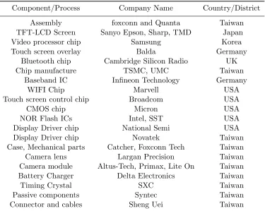
Table 1.1: Suppliers for Apple
Component/Process Company Name Country/District
Assembly foxconn and Quanta Taiwan
TFT-LCD Screen Sanyo Epson, Sharp, TMD Japan
Video processor chip Samsung Korea
Touch screen overlay Balda Germany
Bluetooth chip Cambridge Silicon Radio UK
Chip manufacture TSMC, UMC Taiwan
Baseband IC Infineon Technology Germany
WIFI Chip Marvell USA
Touch screen control chip Broadcom USA
CMOS chip Micron USA
NOR Flash ICs Intel, SST USA
Display Driver chip National Semi USA
Display Driver chip Novatek Taiwan
Case, Mechanical parts Catcher, Foxconn Tech Taiwan
Camera lens Largan Precision Taiwan
Camera module Altus-Tech, Primax, Lite On Taiwan
Battery Charger Delta Electronics Taiwan
Timing Crystal SXC Taiwan
Passive components Syntec Taiwan
Connector and cables Sheng Uei Taiwan
(Apple produces several components as well.) And then, all the components are assembled with respect to Apple’s design and regulations in the factories of Foxconn in China. We list a few main companies related to the i products in the table below. At the same time, each component is assembled by even smaller parts which may exist across different components, such as customized circuit chips, ram, diode, and capacitors made by different materials. These companies are not making everything by their own either. They need materials and even smaller subcomponents from upper stream suppliers, so that they can design and assembly them to manufacture the products Apple requires.
To properly model the assembly manufacturing network, we introduce some notations in Section 1.1, and define four different kinds of nodes in Section 1.2. Specifically, the “source nodes” are used for providing raw materials, “termination nodes” for collecting the final prod-ucts, “ordinary nodes” for the transition of flows and “combination nodes” for assembly or synthesis operations. A linear programming formulation is presented in Section 1.3. This al-lows us to develop a network simplex algorithm for the maximum flow problem in assembly manufacturing networks.
1.1
Preliminaries
In this section we introduce a few definitions and some notations of graph theory and optimiza-tion. For detailed information, please see Ahuja et al. [5], Bazaraa et al. [15], Bertsimas and Tsitsiklis [18], and Lawler [97].
Definition 1.1.1. A graphG= (N, A)is a structure consisting of a finite setN ={1,2, . . . , n}
of elements called nodes and a setA={(i, j),(k, l), . . . ,(s, t)}of unordered pairs of nodes called arcs.
Definition 1.1.2. A path between nodes sand t, or simply an(s, t) path, is a sequence of arcs of the form (s, i1), (i1, i2), . . . , (ik, t), in which the arcs and nodes are distinct.
Definition 1.1.3. An (s, t) path is open if s6=t and closed if s=t. A cycle is an (s, s) path
containing at least one arc, in which no node excepts is repeated.
Definition 1.1.4. Two nodesiand j are connected if there exists an (i, j) path. A graphGis said to be connected if all pairs of nodes are connected.
Definition 1.1.5. A graph G0= (N0, A0) is a subgraph of G= (N, A) if N0⊆N and A0 ⊆A. Definition 1.1.6. A graph is acyclic if it does not contain any cycle.
Definition 1.1.7. A tree in graph Gis a connected acyclic subgraph of G. A spanning tree of
graph Gis a tree that includes every node of the graph G.
When each of the arcs has a direction, we have similar definitions.
Definition 1.1.8. A directed graph G = (N, A) is a structure consisting of a finite set N =
Definition 1.1.9. In a directed graph, for an arc(i, j)∈A, we refer to nodeias the tail node
and j the head node. We say that the arc (i, j) emanates from node i and terminates at node
j. The arc(i, j) is an outgoing arc of nodei and an incoming arc of node j.
Definition 1.1.10. In a directed graph, when there exists an arc (i, j)∈A, we say that nodes
j andi are adjacent to each other and (i, j) is an adjacent arc of nodes i and j.
Definition 1.1.11. In a directed graph, for each nodei∈N, we define
E(i),{j ∈N|(j, i)∈A} (1.1)
to be the “entering” set of node i. The number of nodes in E(i) is the indegree of node i.
Similarly,
L(i),{j∈N|(i, j)∈A} (1.2)
is defined to be the “leaving” set of node i. The number of nodes in L(i) is the outdegree of
nodei. The degree of a node is the summation of its indegree and outdegree.
Definition 1.1.12. In a directed graph G, a directed path from node s to t is a sequence of
distinct arcs from stot, where thepth arc is incident to the same node from which the(p+ 1)st
arc is incident. That is, all arcs are directed from stoward t. A directed (s, t) path is open if
s6=t and closed if s=t. A directed cycle is a nonempty closed directed path.
Definition 1.1.13. A node i is said to be connected to node j if there exists a directed (i, j)
path. If an (i, j) path exists when ignoring the directions of all arcs in this directed graph, we
say nodes i and j are weakly connected. A closed path after ignoring the directions in this
directed graph is called a cycle. A directed graph Gis said to be weakly connected if all pairs of
nodes are weakly connected.
We assume all the graphs in our dissertation are weakly connected.
Definition 1.1.14. A simple directed graph is a directed graph having no multiple arc between
two nodes or loops (an arc emanates and terminates at the same node).
Unless stated otherwise, the term “directed graph” in this dissertation refers to a simple directed graph.
Definition 1.1.15. A direct graphG0 = (N0, A0) is a subgraph of directed graph G= (N, A) if
N0 ⊆N and A0 ⊆A.
Definition 1.1.17. A tree in a directed graph G is a weakly connected acyclic subgraph of G.
A spanning tree in a directed graph G is a tree that includes every node of G.
Definition 1.1.18. A directed graph that contains no cycle is a forest. Alternatively, a forest is a collection of trees.
With all these definitions, we start introducing the assembly network in Section 1.2.
1.2
Assembly manufacturing networks
Suppose that each arc (i, j) of a directed acyclic graphG= (N, A) is assigned a positive number uij, the capacityof (i, j). This capacity is the maximum amount of commodity that can “flow”
through the arc. Such a flow is permitted only in the indicated direction of the arc, i.e., fromi toj. Let
xij = the amount of flow through arc (i, j).
Then, clearly,
0≤xij ≤uij.
LetU be the vector consisting ofuij, ∀(i, j)∈A. We useG= (N, A, U) to represent a network
in which the flow values are between 0 and U.
To model the processes of an assembly manufacturing network, four different types of nodes are defined as follows:
1. Source node (S node for short).
As shown in Figure 1.1,S nodes are source nodes for raw materials. A manufacturing network Ghas at least one source node. EachS node represents one different raw material. We useNS
to denote the set of all S nodes. For each i∈ Ns, E(i) = ∅ and there is an associated input
flow of xi such that
xi=
X
j∈L(i)
xij, ∀i∈NS. (1.3)
We assume only one kind of raw material is allowed at each S node.
…
Figure 1.1: S node
We useNO to denote the set of ordinary nodes where flow balance is maintained, i.e.,
X
k∈E(i)
xki =
X
j∈L(i)
xij, ∀i∈NO. (1.4)
…
…
Figure 1.2: O node
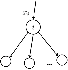
3. Combination node (C node for short).
LetNC denote the set of allC nodes, We can see that in Figure 1.3, for eachi∈NC,
L(i) = {i∗}, (1.5)
xji = kjixii∗, ∀j∈E(i), (1.6)
kji > 0, (1.7)
wherekji is the combination ratio between the incoming arc flow xji and the outgoing arc flow
from i. We denote i∗ as the leaving node of combination node i. For the analysis in later chapters, we call a C node a C= node if P
j∈E(i)kji = 1, a C
− node if P
j∈E(i)kji <1 and a
C+ node if P
j∈E(i)kji >1. Let NC= denote the set of all the C= nodes, NC+ denote the set of
all C+ nodes andNC− denote the set of allC− nodes. Naturally, NC =NC=∪N + C ∪N
−
C.
…
Figure 1.3: C node
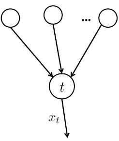
4. Termination node (T node for short).
T node is the termination for the final assembled product or final service supported by the whole network. A T node is shown in Figure 1.4. Our assembly network model has only one termination node. For the termination node t,L(t) =∅ and there associates an output flowxt
such that
xt=
X
i∈E(t)
xit. (1.8)
Similar toS nodes, only one kind of final product is allowed to flow out of a T node.
…
Figure 1.4: T node
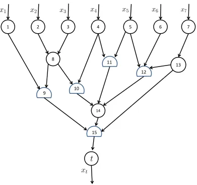
types of nodes. As shown in the figure, nodes 1, 2, 3, 4, 5, 6 and 7 are source nodes, each representing a resource entering the network. Nodes 8, 13 and 14 are the ordinary nodes where materials or semifinished products are transhipped. Nodes 9, 10, 11, 12 and 15 are the combination nodes where assembly or synthesis operations are conducted. Node t is the termination node from which final product exits the whole manufacturing network.
1.3
Model formulation
In an assembly manufacturing network with multiple S nodes and one unique T node, we say xt is the output flow value of the whole network. Our goal is to find the maximum output flow,
such that the capacity constraints on each arc and the ratio requirement at each combination node are satisfied.
Based on the previous descriptions of different types of nodes, our problem can be formulated as:
max xt
s.t.
xi =
X
j∈L(i)
xij, ∀i∈NS (1.9)
X
j∈E(i)
xji =
X
j∈L(i)
xij, ∀i∈NO (1.10)
xji = kjixii∗, ∀i∈NC, j ∈E(i), L(i) ={i∗} (1.11) xt =
X
i∈E(t)
2 3 4 5 6 7 1
12 8
13 11
9 10
14
15 15
0≤xi≤ui, ∀i∈NS
0≤xij ≤uij, ∀(i, j)∈A
0≤xt≤ut,
where for each i∈NS, ui is the maximum amount of raw material ithat source node i could
supply into the network,uij is the capacity of arc (i, j), andutis the capacity of the flow going
out of nodet.
This linear programming formulation contains most of the numerical information in our network; however, some nodes’ tails or heads have not been defined yet. In order to reduce the number of variables of the problem, we can aggregate a group of weakly connected C nodes into a singleCnode, and replace anyO node whose indegree and outdegree are both 1. We will provide specific approaches to standardize and compactify our network model in later chapters.
1.4
Outline of dissertation
Chapter 2
Literature Review
Networks are pervasive in various applications with different settings. Researchers started ana-lyzing network flows from physical networks which are the most common and readily identifiable classes of networks. Among physical networks, the “transportation network” was one of the closest domains to people’s lives and attracted attention of Kantorovich [86], Hitchcock [79], and Koopmans [96]. Their studies provided insight into a transportation problem which was a special case of the minimum cost flow problem and summarized an algorithmic approach. The advent of the simplex method by Dantzig in 1947 raised more interest in network flow problems and Dantzig himself specialized the algorithm for the transportation problem in 1951.
In the past decades, research on network flows was not limited to physical networks in transportation settings; they also involve several other scenarios from applied science and engi-neering, such as mathematics, chemistry, and electrical, communications, mechanical and civil engineering. When networks occur in these various disciplines, their nodes, arcs and flow values model numerous entities. For example, in the telecommunication network, nodes are the places where signals are generated or where the exchanging hubs are located, arcs denote copper or fiber optic cables connecting different nodes, and the flow would signify the transmission of signal or data packages.
Network flow problems also arise in surprising ways for problems that under the surface that might not appear to have any relation to physical networks at all. Problems such as the social network, the page ranking network for web sites searching and software development work flows do not have a physical network, but researchers can abstract the problems into network flow problems.
flow problem is the most fundamental and has numerous applications in practice. The maxi-mum flow problem seeks a feasible solution that sends the maximaxi-mum flow from a specified source nodesto another specified sink node t. In this chapter, we conduct a review of the algorithms for maximum flow problems in traditional network flows, and list a series of representative maximum “flow” applications in Section 2.1; then, in Section 2.2, we review the approaches for network flow problems based on the manufacturing network, which was introduced and defined by Fang and Qi [49].
2.1
Research of traditional maximum flow problem
The traditional maximum flow problem is stated as follows: in a capacitated network, we wish to send as much flow as possible between two special nodes, a source node s and a sink node t, without exceeding the capacity of any arc. We use m to represent the number of arcs, n the number of nodes and ¯U to indicate the maximum flow value. Although the maximum flow problem was posed half a century ago, it is still attractive to researchers seeking more efficient algorithms for its solution. In Section 2.1.1, we review some outstanding algorithms for solving the maximum flow problem, and in Section 2.1.2, a list of applications is provided with refer-ences. Section 2.2 reviews the previous research work related to manufacturing network and Section 2.3 summarizes literature on experimental design and instances generation.
2.1.1 Maximum flow algorithms
The earliest record was dated from 1956, when Ford and Fulkerson [51] formally stated the maximum flow problem. Later Fulkerson and Dantzig [57], Ford and Fulkerson [52] and Elias
et al.[46] gave solutions with proofs of their optimality. To solve the maximum flow problem,
by a sufficient large number.
Edmonds and Karp [45] proved that the labeling algorithm of Fulkerson and Dantzig [57] has a complexity ofO(mU¯) with trivial examples when all the capacities are integral. atahe number of steps cannot be bounded by a function that depends on the the total number of parameters. Edmonds and Karp fixed the original labeling algorithm in the same paper. By imposing the “first labeled first scanned” rule, which is essentially a “breadth first search” on the graph, the revised labeling algorithm augments through the shortest augmenting path, and the maximum flow in the n-node network is obtained after no more than 14(n3−n) augmentations. This new algorithm assured the polynomial computation time ofO(m2n) (in dense graph, m =O(n2)). They further showed that if each flow change is chosen to produce a maximum increase in the flow value, then with integral capacities, a maximum flow would be determined within at most
d1 + logM/(M−1)U¯esteps where M is the maximum number of arcs across a cut.
Independently of Edmonds and Karp, Dinic [43] also discovered the idea of using the short-est augmenting path. But in addition, he found a better platform to carry out this idea. His algorithm is formed by phases. In each phase an auxiliary network is constructed from the given network and the present flow. This network is recorded with layers V0, V1, . . . , Vk, in
whichV0 ={s},Vk={t}, and every one of its arcs goes from one layer to the next layer. v∈Vi
if the shortest augmenting path fromstovis of lengthi. Dinic used the layered network to find enough augmenting paths totwith lengthkuntil every path fromstotin the layered network contains a saturated edge. While Edmonds and Karp exhausted all the shortest augmenting paths in O(m2) steps, Dinic did it with the help of the layered network in O(mn) steps. The
reason is that Edmonds and Karp started from scratch in every iteration when looking for one of the shortest augmenting paths, while Dinic’s layered network helps to keep the information needed for finding one shortest augmenting path. The number of phases of Dinic’s algorithm is bounded by n because at the end of a phase no more augmenting path of lengthk exists, the shortest ones would have size larger than k.
increasing and original augmenting path algorithm into some basic operations. In each oper-ation, it sends maximum flow along one arc instead of the whole augmenting path. Though his algorithm suffers extra computation when excess flows are rerouted, it still beats Dinic’s because of more flow increasing steps in each phase.
Cherkasky [28] combined the methods of Dinic and Karzanov by partitioning the layers into blocks of consecutive layers which were called superlayers. Essentially, Cherkasky applied Karzanov’s preflow to the superlayers, and used Dinic’s method inside the superlayers. This new algorithm could be viewed as a “divide and conquer” strategy. With the advantages from the previous two algorithms, Cherkasky reduced the computation when rerouting the excess flows and came up with a total complexity of O(n2m1/2).
Galil [60] followed the same path with Cherkasky, but used different methods when dealing with the superlayers. For each superlayer, his algorithm maintains a forest, which consists of a collection of node-disjoint trees with roots in the front layer and leaves are exactly all open nodes in the rear layer. The role of the forest is to expedite the push of flow in case no edges are closed. Galil proved his algorithm had a complexity ofO(n5/3m2/3). The improvements of Cherkasky and Galil’s algorithms are the largest when the graph is sparse (n≈m).
Malhotra et al.[100] defined reference node and reference potential of each node so that in each phase of Dinic’s algorithm, the effort of finding the augmenting path is bounded byO(n2). Thus the maximum flow can be obtained with the complexity of O(n3), since there will be at mostn−1 such phases.
Galil and Naamad [61] described anO(mn(logn)2) algorithm improved over Dinic’s method by remembering the paths which were generated after deleting the saturated arcs. The path fragments are stored to save extra computation on path finding. Shiloach [123] came up with a similar result at the same time.
trees find and track the capacities within an O(mlogn) bound per general step. This new al-gorithm preserves additional information of the tree structure with the properties from biased 2-3 trees, which was mentioned in Bentet al. [16].
Shiloach and Vishkin [124] discovered an O(n3) sequential algorithm for maximum flow problem. During an iteration in the previously mentioned preflow-push algorithm, it performs a saturating push after examining a nodei. This nodeimay be still active (i.e., excess preflow can be pushed on layer forwards), the algorithm may choose any other active nodes to push the preflow. Shiloach and Vishkin brought a set LIST as a queue and selected a node i from the front of the LIST, performed pushes from this node, and added newly active nodes to the rear of the LIST. People later called their algorithm as FIFO (first in first out) implementation of the preflow-push algorithm. Besides the sequential result, they revealed a parallel algorithm for finding maximum flow in a directed flow network, and its complexity is O(n3(logn)/p), where p (p≤n) is the number of processors used.
One year later, Tarjan [128] proposed a simplification of Karzanov’s algorithm. He used stacks to contain unblocked, unbalanced and blocked nodes in an increasing order by level. Although the worst case bound remainedO(n3), Tarjan’s change might speed up the algorithm in practice.
While polynomial run time algorithms were constructed, pseudo-polynomial algorithms did not stop its evolving. Gabow [58] gave algorithms for network problems that work by scaling the numeric parameters. Assuming all parameters are integers, Gabow added a parameter ∆ and with respect to a given flow x, defined the ∆-residual network G(x,∆) as a network con-taining arcs whose residual capacity was at least ∆. The algorithm starts with ∆ = 2blog ¯Uc and halves its value in every scaling phase until ∆ = 1. Consequently, this algorithm performs 1 +blog ¯Uc =O(log ¯U) scaling phases. In the last phase, ∆ = 1, so G(x,∆) =G(x). Mixed with the shortest augmenting path algorithm, Gabow’s algorithm achieved a total complexity O(mnlog ¯U).
In 1989, Ahuja and Orlin [6] published their work on maximum flow problem. Their new algorithm performs log ¯U scaling iterations, and pushes flows from nodes with sufficiently large excesses to nodes with sufficiently small excessses while never allowing the excesses to become too large (bounded by the scaling parameter ∆). By doing so, the saturating pushes method has a complexity of O(nm) and the nonsaturating pushes method hasO(n2log ¯U).
Later, Ahuja, Orlin and Tarjan [2] collaborated to reduce the number of nonsaturating pushes again. They used ∆/kas the threshold to define the large excess and small excess, where kwas a constant. A phase consists of repeatedly applying the stack-push/relabel step to a large-excess active node of highest label; a phase ends when there are no large-large-excess active nodes. Their stack scaling algorithm incurs an over all running time ofO(nm+n2log ¯U /log log ¯U) with k= dlog ¯U /log log ¯Ue. With the same technique, they improved Tarjan’s previous wave algo-rithm toO(nm+n2(log ¯U)1/2), and modified the dynamic trees method toO(nm+ log(n2/m) + mlognU¯). Also in 1989, Goldberget al.[68] implemented Goldfarb and Hao [69] ’s network sim-plex algorithm solving maximum flow problem. Goldfarb and Hao managed to get the optimal solution in at most nm pivots and O(n2m) time. Goldberg used an extension of the dynamic tree data structure of Sleator and Tarjan, so that the complexity was reduced to O(nmlogn)
In 1990s, Cheriyan and Hagerup [27] creatively used randomization on maximum flow prob-lem and reduced the probprob-lem to executing a strategy in a certain two person combinatorial game where the payoff reflected the cost of the computation. Later, Alon [10] constructed a family of permutations with a certain pseudo-random property which could be used to derandomize Cheriyan and Hagerup’s algorithm for dense networks. Cheriyan absorbed Alon’s discovery and pushed the complexity from Alon’sO(nm+n8/3logn) toO(n3/logn).
King et al.[91] and King [92] pointed out that Alon’s algorithm paid a cost of a factor of
n2/3/logn on derandomizing the strategies. By slightly modified the rules of the game, they constructed a deterministic strategy which improved the bound on the payoff to within an n factor of the randomized version for any constant . In these two papers, the complexities of the algorithms become O(nm+n2+) and O(nmlogm/nlognn).
bounds using the unit length function. Finally, they gave the algorithm with a complexity of O(min(n2/3, m1/2)mlog(n2/m) log ¯U).
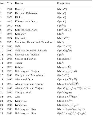
We summarized most of the algorithms and their complexities in the Table 2.1.
Generically, there are five major significant approaches for the maximum flow algorithm from 1950s:
(1) The concept of augmenting path keeps maintains flow balance constraints at every node of the network other than the source and sink nodes. Together with the max-flow min-cut theorem, it offers very natural thinking and mathematical proof for solving the maximum flow problem.
(2) Preflow-push and layered network are the most powerful techniques both theoretically and computationally, and brought the algorithms down to strongly polynomial complexity. They begin with flooding the network so that some nodes would have excesses. The flow decomposition theorem leads the flow to push from source node to sink node and update the distance labels to move the excess backwards.
(3) The dynamic trees data structure provides an efficient way to store and update the network structure. It is the first technique to reduce the computation of retrieval from polynomial order to O(logn).
(4) Scaling, introduced by Gabow [58], implements the pseudo-polynomial bounds for the maximum flow problem with integral capacities. In fact, scaling can be used both in capacities and excess flows. When the optimal value ¯U is polynomially bounded in n, scaling technique plays an important role to shorten the running time and reduce the complexity.
(5) The network simplex algorithm was originally developed by Dantzig in 1951 by specializing his simplex method in network. Although the method itself has a drawback that the worst case of running time can be exponential, researchers have found various ways to improve the rules during pivoting and accelerate it to polynomial complexity. There is also evidence that the network simplex algorithm is computationally among the best for some other network problems. We will include more details about this procedure in Section 2.2.
data structure for storing and operating the network parameters. Basically, it is rearranging parameters of the problem so that the algorithm could benefit from anO(logn) order reduction of the complexity. And it is effective only when implementing other algorithms. The scaling technique is designed for reducing the flow change “step length” by exponentially scaling down the flow capacities. Similar to the dynamic tree, scaling technique is an optional tool to further lower the complexity of an existing algorithm. The network simplex algorithm is a different approach. It has special properties that the graph corresponding to the basis preserves connec-tivity and maintains graphical structure during iterations. Most of the algorithms we described in Section 2.1 computationally benefited from keeping partial information from the previous iterations to avoid unnecessary work. This motivates us to develop an algorithm which could hold network information in each iteration so that we can use it later in more complicated scenarios.
Individually, each of these five major techniques would reduce the computation in a cer-tain phase but incur extra computation in some other aspects. Most of the recent maximum flow algorithms combined several of them and set up detailed strategies under different circum-stances. Thus the description of the algorithms is becoming more complicated while preventing the redundant computation.
The following section will briefly list a few maximum flow applications that researchers have modeled from real world problems. Some of them are mentioned in text books by Ahuja, Mag-nanti, and Orlin [5], Bazaraa et al. [15], and Lawler [97], and some are the ones in which we have great interest. Though the early work of solving the maximum flow problem is largely on transportation and other physical networks, transforming the hidden relationships into maxi-mum flow problems are widely seen in research papers.
2.1.2 Applications
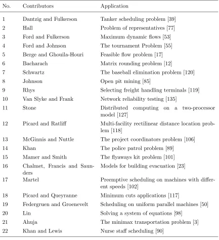
The maximum flow problem arises in a wide range of situations and in several forms. It may be a part of a more difficult network problem, such as the minimum cost flow problem or the generalized flow problem. It could also be related to problems like machine scheduling, assign-ment of computer modules to computer processors and online advertising. In this subsection, we will list a few such applications in Tables 2.2 and 2.3 with corresponding references.
Table 2.1: Complexities of the maximum flow algorithms
No. Year Due to Complexity
1 1951 Dantzig O(nmU)¯
2 1955 Ford and Fulkerson O(nm2)
3 1970 Dinic O(nm2)
4 1970 Edmonds and Karp O(nm2)
5 1970 Dinic O(n2m)
6 1972 Edmonds and Karp O(m2log ¯U)
7 1974 Karzanov O(n3)
8 1977 Cherkasky O(n2m1/2)
9 1978 Malhotra, Kumar and Maheshwari O(n3)
10 1980 Galil O(n5/3m2/3)
11 1980 Galil and Naamad; Shiloach O(nmlog2n) 12 1982 Shiloach and Vishkin O(n3)
13 1983 Sleator and Tarjan O(nmlogn)
14 1984 Tarjan O(n3)
15 1985 Gabow O(nmlog ¯U)
16 1986 Goldberg and Tarjan O(nmlog(n2/m)) 17 1988 Cheriyan and Maheshwari O(n2m1/2) 18 1989 Ahuja and Orlin O(nm+n2log ¯U) 19 1989 Ahuja, Orlin and Tarjan O(nm+n2plog ¯U)
20 1989 Ahuja, Orlin and Tarjan O(nmlog(nplog ¯U /(m+ 2))) 21 1990 Cheriyan et al. O(n3/logn))
22 1990 Alon O(nm+n8/3logn))
23 1992 King et al. O(nm+n2+)
24 1994 King et al. O(nmlogm/nlognn)
Table 2.2: Applications closely related to maximum flow problem.
No. Contributors Application
1 Dantzig and Fulkerson Tanker scheduling problem [39]
2 Hall Problem of representatives [77]
3 Ford and Fulkerson Maximum dynamic flows [53] 4 Ford and Johnson The tournament Problem [55] 5 Berge and Ghouila-Houri Feasible flow problem [17]
6 Bacharach Matrix rounding problem [12]
7 Schwartz The baseball elimination problem [120]
8 Johnson Open pit mining [85]
9 Rhys Selecting freight handling terminals [119]
10 Van Slyke and Frank Network reliability testing [135]
11 Stone Distributed computing on a two-processor
model [127]
12 Picard and Ratliff Multi-facility rectilinear distance location prob-lem [118]
13 McGinnis and Nuttle The project coordinators problem [106]
14 Khan The police patrol problem [89]
15 Mamer and Smith The flyaways kit problem [101] 16 Chalmet, Francis and
Saun-ders
Models for building evacuation [23]
17 Martel Preemptive scheduling on machines with differ-ent speeds [102]
18 Picard and Queyranne Minimum cuts applications [117]
19 Federgruen and Groenevelt Scheduling on uniform parallel machines [50]
20 Lin Solving a system of equations [98]
21 Ahuja The minimax transportation problem [3]
Table 2.3: Applications closely related to maximum flow problem, continued.
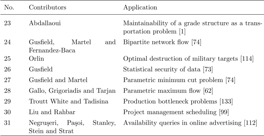
No. Contributors Application
23 Abdallaoui Maintainability of a grade structure as a trans-portation problem [1]
24 Gusfield, Martel and
Fernandez-Baca
Bipartite network flow [74]
25 Orlin Optimal destruction of military targets [114] 26 Gusfield Statistical security of data [73]
27 Gusfield and Martel Parametric minimum cut problem [74] 28 Gallo, Grigoriadis and Tarjan Parametric maximum flow [62]
29 Troutt White and Tadisina Production bottleneck problems [133] 30 Liu and Rahbar Project management scheduling [99] 31 Negru¸seri, Pa¸soi, Stanley,
Stein and Strat
Availability queries in online advertising [112]
in the traditional network flow may no longer exist, such as the max-flow min-cut theorem. However, researchers investigated the connectivity property and used network simplex algorithm to develop adaptive algorithms for manufacturing network flow problems.
2.2
Research on manufacturing networks
Under the settings of manufacturing network flow, the “max-flow, min-cut” theorem not longer holds due to the proportional constraints associated withC and Dnodes. The absence of this important property puts an obstacle when people are trying to use the augmenting path method to get the maximum flow from manufacturing network flow. Since the maximum flow problem is a special case of the minimum cost flow problem, most of the research on manufac-turing network flow is aimed at developing algorithms for minimum cost flow problem based on the network simplex algorithm.
A great advantage of the network simplex algorithm in traditional network is that the linear programming basis of the minimum cost flow problem is a spanning tree, and the algorithm can perform operations on the network itself, without maintaining the simplex tableau or invert-ing any matrices. The network simplex algorithm will always offer an optimal spanninvert-ing tree, which permits us to restrict our search for an optimal solution among spanning tree solutions. The algorithm maintains a spanning tree solution and successively transforms it into an im-proved spanning tree solution until it becomes optimal. A series of research papers confirmed that these tree property and pivoting procedures were able to be adapted from traditional net-work into manufacturing netnet-work structure and efficiently solved several netnet-work flow problems.
Fang and Qi [49] defined a minimum distribution cost problem for a specialized manufac-turing network flow model consisting of D nodes and conventional nodes in their paper. In this model, each D node i has an entering flow xi∗i on its incoming arc (i∗, i), and the flow distillation constraint restricts each flow on its distillation arc (i, j) to be proportional withxi∗i, i.e.,xij =kijxi∗i, wherekij is a constant between 0 and 1. Additionally,P
jkij = 1 and there is
no capacity constraint on each arc. A network simplex algorithm was also proposed in the same paper. However, their method is not complete in the sense that it only describes the algebraic structure of the basis. The procedure lacks detailed steps during flow pivoting. Especially after the identification of branches, the algorithm is still in need of graphical operations for obtaining the initial solution, and updating the flows and dual variables. Besides the minimum cost flow problem, the authors introduced a maximum flow problem for an assembly network, but they did not propose any algorithms to solve the problem.
where the pure network was referred to the traditional network and side constraints/activities were modeling the “subdivisions, refinery activities and assembly”. It is characteristic of their approaches that the pure network part was extracted from the basis. There is an interaction between the “transportation” part and the working basis. The working basis is not fixed, it is dynamic but kept as small as possible. Most of their procedures were conduced with matrix form but not in the network structure.
In particular, Koene [95] introduced a pure processing network containing refining, blend-ing and transportation nodes. Koene proposed his primal simplex method by partitionblend-ing the basis into a transportation forest and representative arcs from the processing nodes. His work revealed several important tree structures which will be used later in our analysis. He also showed that any linear programming problem can be transformed into a pure processing net-work problem and then solved with his primal simplex algorithm. His approach did not fully use the properties of trees and connectivity; relying on matrix multiplication, it still lacks graphical implementation. Chen and Engquist [25] described their primal simplex algorithm in 1986 for pure processing network and did not combine the procedures with network either.
In 1983, Gusfield [72] published his paper studying parametric combinatorial problems with independent parameters. Almost at the same time, Megiddo [107] gave a strong polynomial algorithm for linear programming problems with inequality constraints, where the objective function and each of the constraints depend on at most two variables. Cohen and Megiddo [34] later proved the algorithm to be adaptable to constrained flow problems where the bounds are parametric with fixed number of parameters. However they only showed the existence of such a strongly polynomial algorithm through the reduction from other problems instead of providing detailed operations. Therefore the manufacturing network flow problems are more general and difficult than the previously studied network flow problems and fixed ratio flow problems in the literature. Ahuja et al.[9] studied the simple equal flow problem, a variant minimum cost flow problem requiring each arc in a given subset of arcs must carry the same amount of flow in 1999. Calvete [22], in 2003, extended the simple equal flow problem to a general equal flow problem requiring the flows of arcs on some given sets of arcs to take on the same value. The technique he used is similar to the one from Koene’s paper. He characterized the basis as an (r+ 1)-forest, which included r+ 1 trees, where r indicated the number of the given sets, and finally modified the network simplex method into his primal simplex algorithm.
equals the total amount going out of it. This assumption is reasonable in many applications, especially transportation networks. Many other practical cases, however, violate this assump-tion. Generalized networks (Ahuja, Magnanti, and Orlin [5], Kennington and Helgason [88]) in which each arc has an associated positive multiplier with the flow on it are created to model some of the scenarios violating the arc conservation.
Lu et al. [76] was the first to study the node-conservation-violating case in the minimum
distribution cost flow problem. With the assumption of no capacity on each arc, their work was mainly focused on MDCF≤ and MDCF≥; the former is a minimum distribution cost flow
problem in which allD nodes satisfyingP
j∈L(i)kij ≤1 and the latter is the problem with all
D nodes satisfying P
j∈L(i)kij ≥1. They augmented the existing network by adding pseudo
arcs and nodes for D nodes and converted them into the nodes numerically satisfying flow balance equations. This modification is natural and smooth without scaling or changing the flow value in the existing network. The algorithm in their paper was modified from Fang and Qi’s, so similarly, it is in need of graphical implementations on the pivoting part. Almost at the same time, Sheuet al. [122] developed a type of depth-first-search algorithm using a multi-labeling method which counts and finds all unsaturated subgraphs for solving the maximum flow problem in the distribution network. An advance phase and a retreat phase were defined to find an augmenting structure (most of the time, it is not only a path) in the network. Then every O node whose degree is larger than two in this structure is cut into several sub-nodes to compute the flow increment. The authors did not provide a detailed proof of the algorithm and the complexity analysis is incomplete in the literature. Venkateshan et al.[136] discussed more about the graphical data structures and operations for solving the minimum assembly cost flow problem, and they presented a network-simplex-based algorithm. Their analysis of the problem starts by partitioning the network into suppliers, assemblers and customers layers. This partitioning actually can only represent a special case of assembly network. A concept of general tree was defined in their paper to help them to pivot the basis and change the flow value.
node-conservation-violating case, their framework was still handling the non-violating scenario. And node-conservation-violating examples can easily be made to show that it can not fit into their S-T framework after the transformation described in Luet al. [76].
2.3
Experiments design
Many operations research papers contribute algorithms addressing various applications. A com-mon problem when comparing several algorithms or heuristics is to determine the performance ranking and analyze the factors affecting the performance. There are mainly two points of view regarding to the performance of an algorithm.
1 Theoretical evaluation puts emphasis on the fundamental properties of the algorithms. Worst case analysis and average operations counts describe the limitations of the algo-rithm.
2 Empirical analysis involves programming the algorithm or heuristics in a computer and summarizing the numerical outputs obtained during or after running a group of preset experimenters. CPU time, operation counts are the most typical indices appearing in the literature.
Hall and Posner [78] explained an example that the Simplex method for linear programming has an exponential worst case running time due to Klee and Minty [93]. However, its average running time is polynomial.
Some other authors discuss what should be measured to determine the performance of a solution procedure. These include Crowder and Saunders [35], Hoffman and Jackson [81], Barr
et al.[14] and Ahuja et al.[5]. Hooker [82] made a persuasive case demanding rigorous
com-putational evaluation of algorithms. He suggested the problems be generated in a way that reveals the characteristics of the algorithm. Barret al.[14] commented that the algorithms and heuristics should be tested against the best competitive solution procedures.
Most research studies now use randomly generated problem instances for the testing of algorithms. With the aid from computer, neither the dimension nor the quantity of the exper-imental instances becomes a problem. However, there are no systematic guidelines to generate problems or conduct the evaluations. Independent researchers may come up with totally differ-ent mechanisms for generating instances. Some widely used instances may appear to be very specialized when they are used for algorithms with different objective functions.
Hall and Posner [78] and Amini and Racer [11] proposed some principles to consider when generating test problems.
1 Purpose: Generate data to satisfy the purposes of the experiment.
2 Comparability: Make computational tests comparable.
3 Unbiasedness: Avoid introducing unintended biases into the data. 4 Reproducibility: Make the generation scheme reproducible.
Since there is no previous literature providing numerical results related to the manufacturing network, we will follow these guidelines and generate nondegenerate instances by ourselves. The nondegenerate requirement limits the structure of the assembly manufacture network instances we can generate, thus our purpose is to compare different algorithms’ CPU time and number of iterations needed to reach optimal solution in our specialized assembly manufacturing network experiments.
2.4
Summary
This chapter reviews the literature, and we summarize the previous research work related to our problem. Some major techniques that used for the maximum flow problem in the traditional network were listed in Section 2.1. These studies find that preflow-push algorithms are faster than augmenting path algorithms. With the assistance from dynamic trees which maintain tree structure, algorithms could reduce their complexity at least by an order of log(n). Although the fundamental property “max-flow, min-cut” was not preserved in manufacturing network, it still turns out to be helpful to pivot the flows with respect to the graphical structure instead of barely relying on matrix calculation when deriving algorithm for the maximum flow problem in an assembly network.
in Chapter 7). We start with a standard form which combines the MDCF≤ and the MDCF≥
studied by Luet al.[76] in Chapter 3. And then we modify the network into an S-T circulation framework which was widely seen in the literature solving maximum flow problem in traditional network. Combining the partitioning techniques and the concept of extended cycles from Lu
et al.[75], we give our network simplex algorithm with detailed pivoting procedures in Chapter
5.
Chapter 3
Standard Form Formulation
Although we already have a mathematical formulation of the maximum flow problem in an as-sembly manufacturing network, this formulation is different from the conventional framework. The incoming arcs of the source nodes lack definitions of the tails and there is no head of the outgoing arc of the termination node.
In this chapter we have three objectives. First, in Section 3.1, we bring in two additional nodes and define a few extra arcs to modify the formulation into a traditional S-T circulation framework. Four procedures are provided to reduce the dimension of our problem and avoid the unnecessary computation. An additional procedure is proposed to transform the C− and C+ nodes into C=ones. Then, in Section 3.2, a standard linear programming form of our problem is presented. Section 3.3 uses a real example to illustrate the transformation and preprocessing procedures.
3.1
Transformation
To create an S-T circulation framework similar to the traditional maximum flow analysis, we take the following steps:
(i) add a pseudo source node s0 and an arc (s0, i) as shown in Figure 3.1 to connect s0 to
each source node i∈NS with a flow value capacity of us0i =ui. After taking this step, there is only one source nodes0 in our model, all the previous source nodes are modified
intoO nodes since each of them has the same type of flow balance equation as anOnode.
1 3
2
…
…
…
Figure 3.1: Add a pseudo source nodes0.
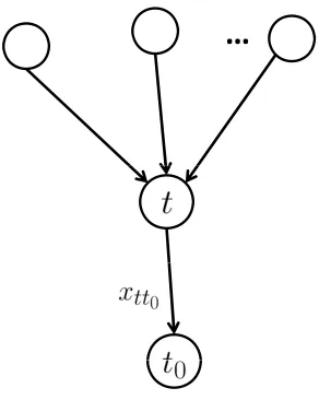
utt0 =ut. Similar to the previous step, nodetis modified to be another O node. We will have only one termination nodet0 from now on.
(iii) add an arc (t0, s0) whose capacity ut0s0 is set to be a sufficiently large number.
After taking these three steps, our model has the same S-T circulation framework as the traditional network. The model is constituted by one source node s0, one termination nodet0,
some ordinary nodes and combination nodes. Each arc in the network has its tail and head nodes well-defined. In the following, four preprocessing procedures are proposed to modify our problem. The Procedures I, II and III prevent unnecessary calculation and reduce the problem size. Procedure IV transforms all theC−and C+nodes intoC= ones by adding an extra adja-cent arc to the combination node together with an additional ratio constraint of the flow values. This transformation guarantees the connectivity property of the basic graph corresponding to a basis. Furthermore, the connectivity property is essential and helpful to develop our network simplex method.
Procedure I If anO nodeiwhose incoming and outgoing degrees are both equal to 1, we denote E(i) ={ie},L(i) ={il}. There are four scenarios that associate with the node type of
il and the status of (ie, il)∈A.
…
Figure 3.2: Add a pseudo sink nodet0.
(ie, i), (i, il) with a single arc connectingieandilwhose capacity is set to be min{uiei, uiil}.
(ii) When the nodeilis anO node and (ie, il)∈A, we remove the nodeiand its adjacent arcs
(ie, i), (i, il), update the capacity of the arc (ie, il) fromuieiltou
0
ieil =uieil+min{uiei, uiil}.
(iii) When the node il is a C node and (ie, il)∈/ A, similar to (i), we replace this node and its
adjacent arcs (ie, i), (i, il) with a single arc (ie, il) connecting ie and il whose capacity is
set to be min{uiei, uiil} and combination ratio is set to bekieil=kiil.
(iv) When the node il is a C node and (ie, il) ∈ A, we remove the node i and its
ad-jacent arcs (ie, i), (i, il), update the capacity of the arc (ie, il) from uieil to u
0
ieil =
min{uiei
kiil
,uiil
kiil
,uieil
kieil
}(kiil +kieil), and the combination ratio of arc (ie, il) is set to be
ki0
eil =kiil+kieil.
Cases (i) and (ii) of Procedure I are illustrated in Figure 3.3 while (iii) and (iv) are shown in Figure 3.4.
Procedure II When two C nodes c1, c2 are adjacent with c2 ∈ E(c1), we merge c2 into
c1 by combining the entering sets of c1 and c2, and update the capacity and the combination
ratio of each incoming arc of the newc1 as follows.
For i = 1,2, we use qi to denote the number of incoming arcs of ci, i.e., |E(c1)| = q1,
|E(c2)| = q2. Let dj, j = 1, . . . , q1−1, be the nodes in the entering set of c1 other than c2;
fj, j= 1, . . . , q2, be the nodes in the entering set ofc2 and E(c01) =E(c1)∪E(c2)\ {c2}. uic0 1 represents the new capacity from nodeito the new combination nodec01 (originalc1), and kic01
(i) (ii)
Figure 3.3: (i) and (ii) of Procedure I.
(iii) (iv)
(i) For a nodei that belongs toE(c1) but not inE(c2)∪ {c2}, let
kic0
1 =kic1 anduic 0
1 =uic1. (ii) For a nodei that belongs toE(c2) but not inE(c1),
kic0
1 =kic2kc2c1 and uic 0
1 =uic2. (iii) For a nodei that belongs to bothE(c1) and E(c2),
kic0
1 =kic1 +kic2kc2c1, uic0
1 = min
uic2
kic2kc2c1 , uc2c1
kc2c1 , uic1
kic1
(kic1+kic2kc2c1).
…
…
…
…
…
…
Figure 3.5: Combine adjacentC nodes.
Procedure II merges adjacentC nodes and reduces the total number of arcs in the network. The preprocessing work would reduce our network into a smaller one as shown in Figure 3.5
Procedure IV For aC nodeiwithP
j∈E(i)kji6= 1, we either add an incoming arc or add
an outgoing arc to make the total flows value coming into theC node equal to the total value going out.
(i) for a C− node i withP
j∈E(i)kji <1, as shown in Figure 3.6, let ks0i = 1−
P
j∈E(i)kji
and add an incoming arc (s0, i) with us0i = ks0iuii∗ +εs0i and an additional constraint xs0i = ks0ixii∗ in which L(i) = {i
∗}. The constant ε
s0i is a small positive real number to keep the arc (s0, i) in the basis. If εs0i = 0, we may have multiply choices when we are searching for the arc to pivot out from the basis, thus a positive εs0i can reduce the chance of degeneracy in pivoting procedures.
(ii) for a C+ node i with P
j∈E(i)kji >1, as shown in Figure 3.7, let kit0 =
P
j∈E(i)kji−1
and add an outgoing arc (i, t0) for node i with uit0 = kit0uii∗+εit0 and an additional constraint xit0 =kit0xii∗ in which {i
∗}=L(i)\ {t
0}. For the same purpose, we add the
positive constantεit0 to prevent degeneracy.
…
Figure 3.6: Modify the C− nodei.
With the Procedure IV, each C node i satisfies the flow balance constraint after the transformation, i.e., P
k∈E(i)xki =Pj∈L(i)xij. All theC− nodes have exactly the same
…
…
Figure 3.7: Modify the C+ nodei.
Each of them has two outgoing arcs and one of these two is an adjacent arc of t0. For
simplicity, we will useC= to specify the originalC= nodes together with transformedC− nodes. Thus in the rest of this thesis, we will only have two types of C nodes, C= and C+, and NC =NC=∪NC+.
3.2
Standard form
After the transformations are conducted in Section 3.1, our network looks like Figure 3.8.
…
…
…
…
max xtt0 s.t.
xt0s0 =
X
i∈L(s0)
xs0i (3.1)
X
j∈E(i)
xji =
X
j∈L(i)
xij, ∀ i∈NO (3.2)
xji = kjixii∗, ∀ i∈NC, j∈E(i), L(i) ={i∗} (3.3) xit0 = kit0xii∗, ∀ i∈N
+
C, L(i) ={i
∗, t
0} (3.4)
X
j∈E(t0)
xjt0 = xt0s0 (3.5)
0≤ xij ≤uij, ∀(i, j)∈A (3.6)
where equations (3.1), (3.2), (3.5) define the flow balance at the nodes0, theO nodes and the
node t0, equation (3.3) is the flow combination ratio constraint associated with each C node
and (3.4) is the additional outgoing flow constraint for the C+ nodes. The constraint (3.6) defines the arc flow bounds. For convenience, we setut0s0, the capacity of arc (t0, s0) equal to
P
i∈L(s0)us0i+ in the modified network, where is a very small positive real number. The summation is slightly more than the maximum flow value permitted to enter the network at the pseudo nodes0. Note that after modification, eachCnode holds the flow balance equation,
which means that equation (3.5) can be derived from other equations and thus it is removable.
With the removal of equation (3.5), a simpler form could be written as max xtt0
s.t.
1 cs0 0 O˜ 0 C˜
x = 0 (3.7)
0≤xij ≤uij ∀(i, j)∈A
wherex= (xt0s0, . . . , xij, . . . , xtt0)
T,
cs0 represents the coefficient vector of the constraint in (3.1), ˜
O is the coefficient matrix regarding to O nodes (including the original source nodes and node t),
˜
C is the coefficient matrix regarding toC nodes, uij is the upper bound for the flow value on arc (i, j).
flow balance equations and then derive pivoting rules in the development of a network simplex algorithm.
3.3
Example
In this section, we use an example to illustrate the preprocessing and transformation in steps. In Figures 3.9, 3.10, 3.11 and 3.12, the number on each arc stands for its capacity, the ratio on the side of the combination node represents the kji values associated with that C node i.
In the left part of Figure 3.9, nodes 1 and 2 are the source nodes, node 3 is an ordinary node and nodes 4, 5, 6 are the combination nodes while at node 4, each unit of product on arc (4,6) requires 23 units of semifinished product from arc (3,4) and 13 unit of semifinished product from arc (2,4); at node 5, each unit of product on arc (5,7) requires 16 unit of semifinished product from arc (1,5) and 12 unit of semifinished product from arc (2,5) and at node 6, each unit of product on arc (6,7) requires 1 unit of semifinished product from arc (4,6) and 23 units of semifinished product from arc (2,6). Node 7 is the termination node. We will continue using these notations when demonstrating our algorithm.
24/5
21/5 21/5 24/5
1 2 21/5 1 2 24/5 21/5 3 4 2 3 2 3 3 4 2 16/5 2 4 16/5 2/3:1/3 5 4 2/3:1/3 16/5 5 4 5 2/3:1/3 6 1:2/3 4 4 5 2/3:1/3 6 1:2/3 1/6:1/2 1/6:1/2 6 4 6 33/10 6
1:2/3 1:2/3 6 6
33/10 7 8 7 8 8
Figure 3.9: Add nodes and arcs to form an S-T framework,M is the capacity of arc (t0, s0).
equa-21/5 21/5 1 2 1 2 24/5 21/5 24/5 21/5 3 4 2 2 3 4 2 3 2 4 16/5 2/3:1/3 4 16/5 2/3:1/3 5 4 5 2/3:1/3 6 1:2/3 4 4 5 2/3:1/3 6 1:2/3 4 1/6:1/2 1/6:1/2 6 33/10 6 1:2/3 6 33/10 6 1:2/3 7 8 7 8
Figure 3.10: Replace ordinary node 3; merge combination nodes 4 and 6.
21/5 21/5 24/5
1 2 1 2
24/5 21/5 21/5 2+ 3 4 3 3 4 3 6’ 16/5 2/3:1 6’ 16/5 2/3:1 6 5 2/3:1 33/10 1/6:1/2 6 5 2/3:1 33/10 1/6:1/2 2/3 6 6 11/5+ 7 8 7 8 11/5+
1 24/5
21/5 21/5 24/5
1 2 2 11/5 3
21/5 21/5 2+ 3 4 3 3 4 3 56/5 6’ 16/5 2/3:1 4 16/5 2/3:1 6 5 2/3:1 33/10 1/6:1/3:1/2 4 5 2/3:1 33/10 1/6:1/3:1/2 2/3 2/3 6 / 6 12/5 7 8 11/5+ 6 8 7
Figure 3.12: Set ε60t
0 =εs05= 1/5,ut0s0 = 56/5 and relabel all the nodes.
tion and each arc has well-defined head and tail nodes. In the linear programming form of our modified problem, our goal is to maximize the “output” value on flow xt0s0 =x67, and
x = {x71, x12, x13, x15, x24, x25, x34, x35, x46, x47, x56, x67},
u = (565 ,215,245,115,3,4,3,165,3310,125 ,6,8). cs0 = (1−1−1−1 0 0 0 0 0 0 0 0)
T, ˜ O =
1 0 0 −1 −1 0 0 0 0 0 0
0 1 0 0 0 −1 −1 0 0 0 0
0 0 0 0 0 0 0 1 0 1 −1
, ˜ C =
0 0 0 1 0 0 0 −2
3 0 0 0
0 0 0 0 0 1 0 −1 0 0 0 0 0 0 0 0 0 0 −2
3 1 0 0
0 0 0 0 1 0 0 0 0 −1
6 0
0 0 1 0 0 0 0 0 0 −1
3 0
0 0 0 0 0 0 1 0 0 −1
are all the parameters in our network problem. In the next chapter, we analyze the connectivity property in our network problem and derive the optimality conditions as the fundamental of our algorithm in Chapter 5.
3.4
Summary
Chapter 4
Optimality Conditions
Following the preprocessing steps described in Chapter 3, now we may transform the original as-sembly network flow problem into its standard form, in which every node holds the flow balance equation and the termination node is connected to the source node to constitute a traditional S-T circulation framework. If we skip the process of transforming the C− and C+ nodes into theC= ones, the network would not have sufficient flow balance equations to construct an S-T
circulation framework. Although Wang and Lin [139] introduced a new way to transform their network flow problem into an S-T circulation framework by adding a new arc (s0, t0) instead of
the arc (t0, s0), the basic feasible graph may no longer be weakly connected when a C+ node
is involved in their framework. Once we lose the connectivity property, decomposing the basis becomes difficult, especially for pivoting. With the flow balance equation at eachCnode in our modified network, we prove the connectivity of the subgraph corresponding to a basic feasible solution of (3.7) in Section 4.1. Section 4.2 then derives the optimality criteria based on the K-K-T optimality conditions for our problem.
4.1
Connectivity and properties
In the traditional maximum flow problem, a basis of a feasible solution corresponds to a span-ning tree so that the network simplex algorithm can easily pivot from one spanspan-ning tree to another. In our problem, the basis is more than just a spanning tree. The basic feasible flow x constitutes a subgraph GB(x) which is composed of a spanning tree and several incoming arcs
of the C nodes. Each arc in the basic feasible flow x is called a basic arc. Suppose there are p nodes inNC and eachC nodeihasqi incoming arcs, withq=Pi∈Ncqi. We say a node is idle,
if no positive flow goes through it. Otherwise, it is active. A subgraph GB(x) constituted by
Now we introduce some properties of the basic feasible graph.
Lemma 4.1.1. Let x be a basic feasible solution of (3.7) andGB(x) be the basic feasible graph
corresponding to x, in which |N|= n, |NC|=p, |NC=|=p=, |NC+|=p+, |E(i)|= qi for each
i∈NC and q+ =Pi∈NC+qi, q= =
P
i∈N=
C qi. We have the following facts:
(i) The number of basic arcs is n+q−p=−1.
(ii) Each C= node i has either q
i or qi+ 1 adjacent basic arcs, and each C+ node j has
either qj+ 1 or qj+ 2 adjacent basic arcs.
(iii) GB(x) is weakly connected and spans all the nodes.
(iv) Any undirected cycle of GB(x) includes at least one C node.
(v) After removingqi−1 basic arcs for eachC= nodeiand removing qj basic arcs for each
C+ node j, GB(x) can be reduced to a spanning tree of G.
Proof. (i) The rank of the constraints in our problem is the sum of the rank of (3.1), which is
1 plus the ranks of matrices ˜O and ˜C. The rank of ˜O is the total number of O nodes in the problem. Since the number of C nodes is p and s0, t0 are neither inNC nor in NO, the rank
of ˜O isn−p−2. Each C= node hasqi combination ratio constraints in the problem but each
C+ node j has q
j + 1 combination ratio constraints. Hence the rank of ˜C is q= +q++p+.
Therefore, in total we have n−p−2 +q=+q++p++ 1 =n+q−p=−1 basic arcs.
(ii) Each C= node i has q
i incoming arcs and one or two outgoing arcs. If two of these arcs
are not in the basis, there are two cases: (a) one of these two is arc (i, i∗), (b) neither of these two is arc (i, i∗). For case (a), in the basis matrix ˜B, the row corresponding to the other arc has no nonzero element, which contradicts the fact that ˜B is nonsingular. As for (b), in the basis matrix ˜B, the two rows corresponding to these two arcs contain one nonzero element in the same column, which contradicts the fact that ˜B is nonsingular. The proof is the same for C+ nodes. Therefore, each C node ihas at most 1 adjacent nonbasic arc.
(iii) Because nodes s0 and t0 are active, all active nodes are weakly connected to s0 and t0
inGB(x). Now assume that some idle nodes are not weakly connected tos0 and t0 in GB(x).
By rearranging the rows and columns, the basic matrix corresponding to x can be written as:
˜
B= B˜1 0 0 B˜2
!
where the square matrix ˜B1 corresponds to the nodes and basic arcs weakly connected to s0
arcs and nodes appear in the rows of ˜B2 would not appear in ˜B1. It is clear that ˜B2 does not
contain the rows corresponding to the adjacent arcs of s0 or t0. And there are two cases for
˜
B2, (a) ˜B2 involves noC node, (b) ˜B2 involves at least oneC node.
(a) If all the nodes involved in ˜B2 are O nodes, each basic arc in the subgraph associated
with ˜B2 would appear twice in the matrix ˜B2, one with coefficient 1 and the other with
coefficient−1. Therefore, the summation of all the rows of ˜B2 is 0, which contradicts the
fact that ˜B is nonsingular.
(b) If at least one C nodei is involved in ˜B2, there are three cases for thisC node.
(b-1) If node i is a C+ node and its adjacent arc (i, t0) is not in the basis, the row that
corresponds to arc (i, t0) has only one nonzero element taking valuePj∈E(i)kji−1
at the column that corresponds to the arc (i, i∗). We multiply this row by −1, so that after the multiplication when summing up the rows of ˜B2 into a row vector, all
the columns associating with the adjacent arcs of nodeiwould be zero.
(b-2) If node i is a C= node without any adjacent nonbasic arc, after summing up the rows of ˜B2 as a row vector, all the columns associated with the adjacent arcs of node
iwould be zero due to the flow balance equation.
(b-3) If nodeiis aC=node with an adjacent nonbasic arc, similar to (b-2), after summing up the rows of ˜B2 as a row vector, all the columns associating with the adjacent arcs
of nodeiwould be zero due to the flow balance equation as well.
This C node i could not be a C+ node with (i, t0) being a basic arc at the same time,
otherwise it is weakly connected witht0 inGB(x).
After the basic row operations on matrix ˜B2, its row sum becomes zero. This also
con-tradicts the fact that ˜B is nonsingular.
According to (ii), all of the C nodes are in GB(x). If GB(x) does not span all the nodes,
there would exist an O node not weakly connected with GB(x). Thus in the basis matrix, the
row corresponding to this node only contains zeros, which again makes ˜B singular.
(iv) Suppose that there is an undirected cycle inGB(x) that contains no C node. Consider the
submatrix ˜BC of ˜B corresponding to the arcs in this undirected cycle. Note that the rows of
˜
BC corresponding to the combination ratio constraints are all zeros. Hence, the columns of ˜BC
are linearly dependent, which contradicts that ˜B is nonsingular.
one C node. Since each C= node i has at least qi adjacent basic arcs and each C+ node j
has at least qj + 1 adjacent basic arcs, if we remove qi−1 basic arcs for each C= node i and
remove qj basic arcs for each C+ node j from GB(x), then the remaining subgraph contains
n−1 basic arcs and remains weakly connected without any undirected cycle. The remaining subgraph becomes a spanning tree of thesen nodes.
Although Lemma 4.1.1 appears similar to the properties proposed by Fang and Qi [49], they are not identical in the following sense: We generalized the results from uncapacitated case to the capacitated one, and suggest a transformation and a mathematical model to keep the connectivity and handle the situation when there are no flow balance equations with C nodes. The description of properties (iv) and (v) will help us derive the optimality conditions in Section 4.2 and design the algorithm in Chapter 5.
As an example, a basic feasible graph of the example we showed in Chapter 3 is displayed in Figure 4.1.
1
3 2
4 5
6
7 7