Comparison of SGA and RGA based Clustering Algorithm for Pattern Recognition

Comparison of SGA and RGA based Clustering

Algorithm for Pattern Recognition

Kumar Dhiraj,

Dept of Computer science and Engineering,

National Institute of Technology Rourkela Rourkela, Orissa, INDIA

Email id: [email protected]

Santanu Kumar Rath

Dept of Computer science and Engineering,

National Institute of Technology Rourkela Rourkela, Orissa, INDIA

Email id: [email protected]

Abstract--- In this paper Genetic Algorithm based clustering Algorithm has been studied for pattern recognition. The searching capability of genetic algorithms is exploited in order to search for appropriate/optimal cluster as well as cluster’s center in the feature space such that inter-cluster distance (Homogeneity) and intra-cluster distances (Separation) are optimized. We use H-S ratio for computation of fitness function. We use Anderson’s IRIS data to illustrate our method. We have implemented six clustering algorithm (k-means, Hierarchical, GLVQ, SOM, FCM and GA-based clustering algorithm) and compare clustering accuracy using IRIS data.

Index Terms—K-means, Hierarchical clustering, GLVQ, SOM, FCM, GA, Homogeneity and Separation, Iris.

I. INTRODUCTION

Genetic algorithm (GA) is inspired by Darwin’s theory of evolution. A GA works with a population of individuals each of which represents a potential solution to the problem to be solved. A typical individual is a binary string on which the problem solution is encoded. Problem representation is one of the key decisions to be made when applying a GA to a problem. How a problem is represented in a GA individual determines the shape of the solution space that a GA must search. As a result,

different encodings of the same problem are essentially different problems for a GA [1]. The application of Gas for solving problems of pattern recognition appears to be appropriate and natural. Research articles in this area have started to come out [2], [3]. An application of GAs has been reported in the area of (supervised) pattern classification in RN for designing a GA-classifier [4], [5]. When the data available are unlabelled (i.e. test data or Reference data are not available), the classification (supervised) are referred to as unsupervised classification i.e. clustering. Clustering [6-9] is an important unsupervised classification Techniques which has been described in the next section in details. GA based Clustering algorithm has been also reported in the previous work [10].

In this paper we have presented GA with a four different representation scheme. We use binary representation (SGA-Simple Genetic Algorithm) as well as floating-point representation (RGA-Real coded Genetic Algorithm) for GA. It is important to note that

efficiency of a GA based algorithm mainly depends on two factors: first representation scheme and Fitness function computation [11], [12]. The way we have represented a chromosome in GA and use of a novel fitness function (H-S ratio) makes it different from previous approaches and results in a highly efficient algorithm.

II. CLUSTERING

The clustering problem is defined as the problem of classifying n objects into K clusters without any a priori knowledge. Let the set of n points be represented by the set S and the K clusters be represented by C ,C , … , C

.

ǿ

1,2, … , ,

Ǿ 1, … , , 1, … ,

.

In recent years, a number of clustering methods have been proposed [9], [13], [14], [15]. In this section, we will explain about five different techniques and how we can exploit it for data clustering.

A.K-Means

The K-means algorithm [8], one of the most widely used clustering techniques. The steps of the K-means algorithm are described in brief as follows:

Note that in case the process does not terminate at Step 4 normally, then it is executed for a maximum "fixed number of iterations”. It has been shown in Ref. [16] that K-means algorithm may converge to values that are not Step 1: Choose initial cluster centers , , … , randomly from the points , , … , .

Step 2: Assign point , 1,2, … , . to cluster , .

Є 1,2, … , , ,

1,2, … , , . Ties are resolved arbitrarily.

Step 3: Compute new cluster centers , , … , as follows: ∑ Є 1,2, … , ,

Where = is the number of elements belonging to cluster . Step 4: If = , , i=1,…,K then terminate. Otherwise repeat from step 2.

270 

optimal. Also global solutions of large problems cannot be found with a reasonable amount of computation effort [17]. It is because of these factors that several approximate methods are developed to solve the underlying optimization problem.

In the next section we will discuss a clustering methodology which will not assume any particular un-derlying distribution of the data set being considered and it should be conceptually simple like the K-means algorithm. On the other hand, it should not suffer from the limitation of the K-means algorithm which is known to provide sub optimal clustering’s depending on the choice of the initial clusters [16], [17].

III. CLUSTERING USING GENETIC ALGORITHM

A. Basic principle

The searching capability of GAs has been used in this article for the purpose of appropriately determining a "fixed number K” of cluster centers in RN; thereby suitably clustering the set of n unlabelled points. The clustering metric that has been adopted is the Euclidean distances of the points from their respective cluster centers. Mathematically, the clustering metric μ for the K clusters C , C , … , C is given by, μ , , … ,

=

∑

∑

||

||

The task of the GA is to search for the appropriate cluster centers z , z , … , z

B. GA Based Clustering Algorithm

The basic steps of GAs, which are also followed in the GA-clustering algorithm, are now described in details in this section. In this section we will discuss about four different representation schemes for encoding of a chromosome.

Representation 1(R1): BGA (Binary coded Genetic Algorithm)

Each chromosome is a sequence of binary numbers representing the clusters. For m data-point of N-dimensional space and ‘K’ number of clusters, the length of a Chromosome will be m*K bits/positions, where the first m positions represent the first cluster the next m positions represent those of the second cluster, and so on. Note that in a cluster if a bit position is “1” (It is said to be in ON state), it means that the data point is present and “0” (It is said to be in OFF state) means data point is absent. As an illustration for the above representation, let us consider the following example.

Example 1.

Consider Iris data [150 x 4], we have m=150, N"4 and K"3, i.e., the space is four dimensional and the number of clusters being considered is three. Therefore, the size of the Chromosome will be 450 (i.e. m*K). Then the Chromosome/String representation will be:

First Cluster Second Cluster Third Cluster

100001... upto150 bits 011000... upto150 bits 000110... upto150 bits

Fig. 3.2.1. Encoding of chromosome using representation 1

According to above chromosome representations (Fig. 3.2.1): since in first cluster index 1 and 6 are one. Therefore, Data point 1 and Data point 6 are presents in First Cluster. Similarly Second Cluster contains Data point 2 and Data point 3, Third Cluster contains Data point 4 and Data point 5, and so on.

Representation 2(R2): RGA (Real coded Genetic Algorithm)

Each Chromosome is a sequence of real numbers representing the centers of K clusters. For m data-point of N-dimensional space, the length of a Chromosome will be N*K bits/positions, where the "first N positions (or, genes) represent the "center of first cluster, the next N positions represent those of the centre of second cluster, and so on. Note that cluster center is of N-dimensional space. As an illustration for the above representation, let us consider the following example.

Example 2.

Consider the same Iris data again. The size of the Chromosome in this case will be twelve (i.e. N*K=12). Then the Chromosome/String representation will be

Center of First Cluster Center of Second Cluster Center of Third Cluster

5.2 4.1 1.5 0.1 5.3 3.7 1.5 0.2  5.7 2.9 4.2 1.3 

Fig. 3.2.2. Encoding of chromosome using representation 2

C. Population initialization

The K clusters encoded in each chromosome are initialized as stated in representation section of chromosome. The chromosome initialization can be done randomly or we can use any greedy or intelligent method to explore it. This process is repeated for each of the P chromosome in the population, where P is the size of the population.

D.Fitness Evaluation

This is the one of the most important part of our method. The fitness function evaluation is based on Homogeneity and separation value. It is based on the principle “objects within one cluster are assumed to be similar to each other, while objects in different clusters are dissimilar”. Fitness computation process consists of two steps: in first step, we calculate Homogeneity value and Separation value and in second step we define H-S ratio. H-S ratio is nothing but ratio of homogeneity to separation.

The homogeneity of a cluster is defined by some measure which quantifies the similarity of data objects in the cluster C. For example,

∑ _{Є ,} .

This definition represents the homogeneity of cluster C by the average pair-wise object similarity within C.

271 

Cluster separation is analogously defined from various perspectives to measure the dissimilarity between two clustersC , C . For example,

,

∑ _{Є Є} .

Since these definitions of homogeneity and separation are based on the similarity between objects, the quality of C increases with higher homogeneity values within C and lower separation values between C and other clusters. Once we have defined the homogeneity of a cluster and the separation between a pair of clusters, for a given clustering result C ,C , … , C , we can define the homogeneity and the separation of C. For example, Sharan et al. [19] used definitions of

H

∑ _Є .

and

∑ . ∑ . ,

to measure the average homogeneity and separation for the set of clustering results C. now we define H-S ratio as ratio of Homogeneity to separation, H S ratio H

S . It is important to note that higher the H-S ratio value, the good is the clustering algorithm.

E. Selection

The selection step in Genetic Algorithm selects chromosome from the mating pool and follows “the survival of the fittest” concept of Darwin’s natural genetic system. In this article, a proportional selection strategy has been adopted. Roulette wheel selection is one common technique that implements the proportional selection strategy. According to this, a chromosome is assigned a number of copies, which is proportional to its fitness in the population that goes into the mating pool for further genetic operations.

F. Crossover

It is a type of genetic operations, which is used to create new child chromosomes from parent chromosomes after exchanging information between them. It is based on probabilistic model. Several variants of Cross-over has been discussed in past. In this article single-point crossover with a fixed crossover probability Pc is used. For chromosome of length

c

the crossover point, is generated in the range [2,

c

The portions of the chromosome lying to the right of the crossover point are exchanged to produce two offspring. G. Mutation

Each chromosome undergoes mutation with a fixed probability, pm. For binary representation of a chromosome we do mutation by flipping its bit position(or gene) value i.e. if a bit position is 1 we have

made 0 and vice versa. For Real coded Genetic algorithm we have done mutation as follows [10]: A random number η in the range [0, 1] is generated with uniform distribution. If the value at a gene position is , after mutation it becomes 1 2 η . One may note in this context that similar sort of mutation operators for real coding have been used mostly in the realm of evolutionary strategies [20].

H.Termination criterion

In this article the processes of fitness computation, genetic operation is executed for a maximum number of iterations.

The next section provides the experimental result performed using GA based clustering algorithm. We have also shown its comparison with K-means algorithm for iris datasets. In last we have shown the percentage of accuracy obtained for iris data using both algorithms.

IV. EXPERIMENTAL WORK

To validate the feasibility and performance of the propose approach, we implemented the approach in MATLAB 7.0(Intel C2D processor, 2.66GHz, 2 GB RAM) and applied it to iris data.

A.Experimental Setup 

Iris data

The IRIS data set [18] is a well known and well used benchmark data set used in the machine learning

community. The dataset consists of three varieties of Iris, Setosa, Virginica and Versicolor. The size of the data is [150 x 4].The characteristic of this data is it’s having some overlap between classes 2 and 3. The original data can be obtained from UCI repository websites

(http://archive.ics.uci.edu/ml/datasets/Iris).

B. Parameter used for GA 

We use crossover probability in the range 0.6 to 0.8 and mutation probability in the range .001 to .01. We also use number of iteration to complete GA in the range 15 to 50.

C.  Results and Discussion 

Table 4.1 summarizes result of all six clustering algorithm for IRIS data. It also represents the best case analysis of four representation schemes used for GA based clustering algorithm. Note that for IRIS data a clustering algorithm which gives less than 18 count errors considered to be a good clustering algorithm [14]. We have achieve count error in the range {0 – 10}. We can easily infer from Table 4.1 that GA based clustering algorithm performs better than all other algorithm for IRIS data. It is important to note that Representation 3 based GA–clustering algorithm can achieves 100 percent accuracy in its best case analysis. It can be easily infers from the table 4.1 that GA based clustering algorithm performs better than other non-GA based clustering algorithm for IRIS data.

TABLE 4.1

  272  Algorithm Coun t Error Percentage error Percentage Accuracy Hierarchical 48 32 68 SOM 22 14.67 85.33 K-Means 17 11.33 88.67 GLVQ 16 10.76 89.33 FCM 14 9.33 90.67 GA(Representation 1) 10 6.67 93.33 GA(Representation(2) 6 4 96

Table 4.2 describes the result obtained by representation 1 based GA. It shows the initial cluster (randomly taken from initial population) as well as final clusters. We have got count error as 10(i.e. percentage accuracy is 93.33%).

Table 4.3 describes the details of Details of Data points wrongly clustered by representation 1 based Ga-Clustering algorithm. Here clustering result for IRIS-setosa is 100 percent whereas in case of Iris-versicolor and Iris-virginica number of data points wrongly clustered is 1 and 9 respectively. Datapoint {78} which should be in versicolor is wrongly clustered into Iris-virginica and datapoint {102, 107, 114, 120, 122, 134, 139, 143, 147} which should be in Iris-virginica is wrongly classified into Iris-versicolor.

TABLE 4.2

INITIAL AND FINAL CLUSTER FOR REPRESENTATION R1 Initial cluster

Cluster1 Cluster2 Cluster3

1 2 3 4 5 6 7 8 9 10 11 12 13 14 15 16 17 18 19 20 21 22 23 24 25 26 27 28 29 30 31 32 33 34 35 36 37 38 39 40 41 42 43 44 45 46 47 48 49 50 53 78 101 103 104 105 106 108 109 110 111 112 113 116 117 118 119 121 123 125 126 129 130 131 132 133 135 136 137 138 140 141 142 144 145 146 148 149 51 52 54 55 56 57 58 59 60 61 62 63 64 65 66 67 68 69 70 71 72 73 74 75 76 77 79 80 81 82 83 84 85 86 87 88 89 90 91 92 93 94 95 96 97 98 99 100 102 107 114 115 120 122 124 127 128 134 139 143 147 150 Final Cluster

Cluster1 Cluster2 Cluster3

51 52 53 54 55 56 57 58 59 60 61 62 63 64 65 66 67 68 69 70 71 72 73 74 75 76 77 79 80 81 82 83 84 85 86 87 88 89 90 91 92 93 94 95 96 97 98 99 100 101 103 104 105 106 108 109 110 111 112 113 115 116 117 118 119 121 123 124 125 126 127 128 129 130 131 132 133 135 136 137 138 140 141 142 144 145 146 148 149 150 1 2 3 4 5 6 7 8 9 10 11 12 13 14 15 16 17 18 19 20 21 22 23 24 25 26 27 28 29 30 31 32 33 34 35 36 37 38 39 40 41 42 43 44 45 46 47 48 49 50 Count error= 10 Accuracy = 93.33 % TABLE 4.3

RESULT OF IRIS DATA USING GENETIC ALGORITHM R1

Iris-setos a Iris-versi color Iris-virginica Total The right number of data point 50 50 50 150 Details of Data points wrongly clustered NIL 78 102 107 114 120 122 134 139 143 147 78 102 107 114 120 122 134 139 143 147 number of data point wrongly clustered 0 1 9 10 number of data point correctly clustered 50 49 41 140 Accuracy (%) 100 98 82 93.33

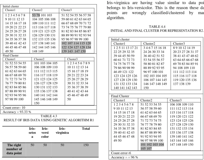
Table 4.4 to Table 4.5 describe the result obtained by representation 2 based genetic algorithms. Table 4.4 show the details of the cluster obtained before and after GA run. Count error we have got as 6. We have achieved 100 % accuracy for cluster Iris-setosa and Iris-versicolor whereas for Iris-virginica we have achieved 88%. The wrongly clustered data points are {101, 102, 103, 104, 105, and 107}. In actual practice, all these data points belong to Iris-virginica but they have wrongly clustered into Iris-versicolor.

Another very important point to be note is that data point {102, 107} is wrongly clustered by both representation R1 and R2. These data point are highly non-separable. Data point 102 is having feature value {5.8, 2.7, 5.1, 1.9} and Data point 107 is having feature value {4.9, 2.5, 4.5, 1.7}. these data point which are in Iris-virginica are having value similar to data point belongs to Iris-versicolor. This is the reason these data points are wrongly classified/clustered by many algorithm.

TABLE 4.4

INITIAL AND FINAL CLUSTER FOR REPRESENTATION R2. Initial cluster

Cluster1 Cluster2 Cluster3

1 2 5 11 13 17 21 22 25 29 32 35 39 44 45 50 59 60 61 71 72 73 74 75 76 77 78 79 86 90 98 99 46 49 121 122 123 124 125 126 127 128 129 130 131 132 133 134 140 141 142 143 3 4 6 7 15 16 18 24 26 30 33 34 36 40 42 51 52 53 54 55 56 57 58 80 81 82 87 88 89 92 93 95 96 97 100 101 102 103 104 105 106 107 144 145 146 147 148 149 150 8 9 10 12 14 19 20 23 27 28 31 37 38 41 43 47 48 62 63 64 65 66 67 68 69 70 83 84 85 91 94 108 109 110 111 112 113 114 115 116 117 118 119 120 135 136 137 138 139 Final Cluster

Cluster1 Cluster2 Cluster3 1 2 3 4 5 6 7 8 9 10 11 12 13 14 15 16 17 18 19 20 21 22 23 24 25 26 27 28 29 30 31 32 33 34 35 36 37 38 39 40 41 42 43 44 45 46 47 48 49 50 51 52 53 54 55 56 57 58 59 60 61 62 63 64 65 66 67 68 69 70 71 72 73 74 75 76 77 78 79 80 81 82 83 84 85 86 87 88 89 90 91 92 93 94 95 96 97 98 99 100 101 102 103 104 105 107 106 108 109 110 111 112 113 114 115 116 117 118 119 120 121 122 123 124 125 126 127 128 129 130 131 132 133 134 135 136 137 138 139 140 141 142 143 144 145 146 147 148 149 150 Count error=6 Accuracy = = 96 %

273  TABLE 4.5

RESULT OF IRIS DATA USING GENETIC ALGORITHM R2.

Iris-setos a Iris-versic olor Iris-virginic a Total

The right number of

data point 50 50 50 150 Details of Data points wrongly clustered NIL NIL 101 102 103 104 105 107 101 102 103 104 105 107 number of data point wrongly clustered 0 0 6 6

The number of data point correctly clustered

50 50 44 144

Accuracy (%) _{100 100 88 96}

Table 4.6 describe the result obtained by representation 3 based genetic algorithms. It shows the details of the generated cluster before as well as after GA run. In this case we achieve 100% accuracy.

We have run GA for all representations 20 times and Summary of results obtained have been shown in Table 4.7.

TABLE 4.7

ANALYSIS OF BEST CASE, AVERAGE CASE AND WORST CASE FOR GA

Representation R1

Best case Average Case Worst case

Count error 10 12 14

Accuracy (%) 93.33 92 90.67

Representation R2

Best case Average Case Worst case

Count error 6 6 6

Accuracy (%) 96 96 96

V. CONCLUSIONS

The GA-based clustering algorithm is a distinct improvement from the non GA-based clustering algorithm. Its ability to cluster independent of the data sequence provides a more stable clustering result. When compared to other known clustering algorithms such as the k-means, Hierarchical, GLVQ, SOM, and FCM, GA based clustering algorithm is superior. As seen from the IRIS data experiments, the GA based clustering algorithm was able to provide the highest accuracy and generalization results. It is also important to note that RGA Performs better compare to SGA.

REFERENCES 

[1]. K. Mathias and L. D. Whitley, “Transforming the search space with gray coding,” in Proc. IEEE Int. Conf. Evolutionary computation, pp. 13–518, 1994.

[2]. E.S. Gelsema (Ed.), Special Issue on Genetic Algorithms, Pattern Recognition Letters, vol. 16(8), Elsevier Sciences Inc., Amsterdam, 1995.

[3]. S.K. Pal, P.P. Wang (Eds.), Genetic Algorithms for Pattern Recognition, CRC Press, Boca Raton, 1996.

[4]. S. Bandyopadhyay, C.A. Murthy, S.K. Pal, “Pattern classification using genetic algorithms”, Pattern Recognition Lett. 16, 801-808, 1995.

[5]. S.K. Pal, S. Bandyopadhyay, C.A. Murthy, Genetic algorithms for generation of class boundaries, IEEE Trans. Systems, Man Cybernet. 28, 816-828, 1998.

[6]. M.R. Anderberg, Cluster Analysis for Application, Academic Press, New York, 1973.

[7]. J.A. Hartigan, Clustering Algorithms,Wiley, New York, 1975

[8]. A.K. Jain, R.C. Dubes, Algorithms for Clustering Data, Prentice-Hall, Englewood Cliffs, NJ, 1988.

[9]. J.T. Tou, R.C. Gonzalez, Pattern Recognition Principles, Addison-Wesley, Reading, 1974.

[10].Maulik, U. and Bandyopadhyay, S., “Genetic Algorithm-Based Clustering Technique,” Vol. 33, pp. 1197-1208, 2002.

[11].A. Clark and C. Thornton, “Trading spaces: Computation, representation, and the limits of uninformed learning,” Behavioral and Brain Sciences, vol. 20, pp. 57–90, 1997. [12].T. Jones and S. Forrest, “Fitness distance correlation as a

measure of problem difficulty for genetic algorithms,” in Proc. 6th Int. Conf. Genetic Algorithms, L. J. Eshelman (ed.), 1995.

[13].T.Kohonen, ”Self-organization and Associative Memory,” Berlin, Germany:Springer Verlag, 1989, 3rd ed:.

[14].N.R.Pa1, J. C. Bedzek and E. C. -K. Taso, ”Generalized Clustering Networks and Kohonen’s Self- Organizing Scheme,” IEEE Trans. on Neural Networks, Vol. 3, No. 4, pp.546-557, July 1993.

[15].J. C. Bezdek, E. C. K. Taso and N. R. Pal, ”Fuzzy Kohonen Clustering Theorem,” Proceeding of IJCNN, pp.1035-1041, 1992.

[16].S.Z. Selim, M.A. Ismail, K-means type algorithms: a generalized convergence theorem and characterization of local optimality, IEEE Trans. Pattern Anal. Mach. Intell. 6, 81-87, 1984.

[17].H. Spath, Cluster Analysis Algorithms, Ellis Horwood, Chichester, UK, 1989.

[18].E. Anderson, “The IRISes of the Gaspe Penisula,” Bulletin of the American IRIS society, vol. 59, pp. 2-5. 1939. [19].Shamir, R. and Sharan, R. Click: A clustering algorithm

for gene expression analysis. In Proceedings of ISMB '00, pages 307-316, 2000.

[20].Z. Michalewicz, Genetic Algorithms+Data Structures" Evolution Programs, Springer, New York, 1992.