CONSCIOUS AWARE ROUTING PROTOCOL FOR MOBILE WIRELESS SENSOR
NETWORKS
Vijayasathana.K
M.E(Computer Science and Engineering) KPR Institute of Engineering and Technology
Arasur,Coimbatore.
Vishnukumar.k,Ph.D., Computer Science and Engineering KPR Institute of Engineering and Technology
Arasur,Coimbatore.
Abstract— Conscious aware routing protocol is a novel
solution to routing. improving route discovery, network performance and reducing the mobility of the node . For data transmission, the network topology is the major significant for selecting the route to transmits the data packets to reach the destination . The greatest challenges were raised in network topology of mobile wireless sensor networks to route the data from source to destination. Therefore, the routing protocols should have the location information of the nodes and less energy consumption and latency. In this paper, conscious aware routing protocol is proposed for improving the network performance. conscious score of each node is calculated by trust value, link quality, remaining energy and variation based distance metric-Mahalanobis distance. The link quality of the node is estimated by using RSSI technique which is utilized for reducing the packet loss. Finally, the results proves that the network performance is improved.
Keywords – Route discovery , Location information,Trust aware routing, Conscious score, Trust value, Network performance.
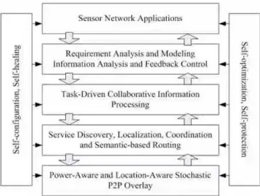
1) INTRODUCTION
The topic of wireless sensor networks (WSNs) has recently gained a lot of research interest due to the availability of low cost, low power transmitters, making it cost effective to create small networks of sensors. These sensors are typically radio enabled nodes with simple transducers connected to a microcontroller. Sensor networks use numerous small, inexpensive nodes that can sense, compute, and communicate with each other to interact with the physical world. sensor network configuration may require consideration of aspects of the physical environment. For these reasons, automatic configuration of a sensor network is both essential and challenging. Nodes in sensor networks interact closely with their surrounding environment, and one of the most important parameters in many sensor network applications is location. Introduce two main innovations, which work cooperatively to respond to attacks in the wireless network: a lightweight solution for accurate localization information based on range-free techniques (for radio access networks where only the RSSI information is available), and an innovative trust-aware routing approach called Ambient Trust Secure Routing (ATSR) protocol which is based on the geographical routing principle and incorporates a distributed trust model to defend against routing attacks. Accurate localization information is necessary both for application layer Intrusion Detection
Systems (to identify/locate the intruders) and for secure routing since the proposed location-based routing requires trustable localization information. It is worth pointing out that a geographical routing approach has been adopted to efficiently cope with the large network.
2) REVISED OPTIMIZATION TECHNIQUE FOR TRUST AWARE ROUTING:
2.1) Ad-hoc on-demand distance vector routing protocol
Adhoc On Demand Distance Vector Routing AODV a novel algorithm for the operation of such adhoc networks. Each Mobile Host operates as a specialized router and routes are obtained as needed on demand with little or no reliance on periodic advertisements. Their new routing algorithm is quite suitable for a dynamic self starting network as required by users wishing to utilize adhoc networks AODV provides loop free routes even while repairing broken links.Their main objective of this work is to broadcast discovery packets only when necessary. Then distinguish between local connectivity management neighborhood detection and general topology maintenance.
2.2) A geographically opportunistic routing protocol
Geographically Opportunistic Routing protocol (GOR) is designed. In GOR, the bounded sensor area is divided into unchangeable grids at the initialization of a network. Each grid has its priority according to its distance to the sink. All nodes having received the packet determine their priorities according to which grid they lie in and the starting grid included at the head of the packet. Then they listen to ACK for this packet and wait for their turns. In the packet forwarding to the next candidate, the information of the starting grid is updated. This process is repeated until the packet reaches the sink. For each transmission, once several nodes in the same grid have received the packet, they compete to be the only forwarding node.
2.3) Energy efficient communication protocol
LEACH (Low-Energy Adaptive Clustering Hierarchy), a clustering-based protocol that utilizes randomized rotation of local cluster base stations (cluster-heads) to evenly distribute the energy load among the sensors in the network. LEACH uses localized coordination to enable scalability and robustness for dynamic networks, and incorporates data fusion into the routing protocol to reduce the amount of information that must be transmitted to the base
station. Thus, communication between the sensor nodes and the base station is expensive, and there are no “high-energy” nodes through which communication can proceed.
2.4) Self-organization routing protocol
The basic idea in LEACH-Mobile is to confirm whether a mobile sensor node is able to communicate with a specific cluster head, as it transmits a message which requests for data transmission back to mobile sensor node from cluster head within a time slot allocated in TDMA schedule of a wireless sensor cluster.
Figure 2.1- self optimization routing protocol
The LEACH-Mobile protocol achieves definite improvement in data transfer success rate as mobile nodes Proceedings of increase compared to the non-mobility centric LEACH protocol. Mobility centric protocol for wireless sensor network that support mobile nodes for typical environment of 'hot area'.
2.5) Mobility-based clustering protocol
The proposed protocol will take an estimated connection time into account in order to build a more reliable path depending on the stability or availability of each link between a non-cluster-head sensor node and a cluster head node. In the MBC protocol, a node elects itself as a cluster head based not only on its residual energy but also on its mobility in order to achieve balanced energy consumption among all nodes and thus longer lifetime of the network. The non-cluster-head nodes send data packets according to the time schedule. It will broadcast a joint request message in order to join a new cluster and avoid more packet loss.
3) LOCALIZATIONTECHNIQUESUSEDINWSN
3.1) Location aware routing protocols for WSN
Location aware routes are set by node locations. The space is divided into quadrants. Each node knows its position in space (e.g., GPS). To focus the physical coordinates of a gathering of sensor nodes in a wireless sensor network (WSN).
Because of application context, utilization of GPS is unrealistic; consequently, sensors need to self-organize a coordinate system. All in all, just about all the sensor network localization algorithms impart principally three basic stages. They are:
Distance Estimation Position Computation Localization Algorithm
In location-based protocols, sensor nodes are simply addressed by their means of locations. In sensor networks, location information for nodes is necessary. To estimate energy consumption, all the routing protocols should calculate
the distance between two particular nodes. We present a brief about location-aware routing protocols in WSNs.
3.2) Geographic Random Forwarding (GeRaF):
GeRaF uses geographic routing where a sensor acting as relay is not known a priori by a sender. There is no guarantee that a sender will always be able to forward the message toward its ultimate destination, that is, the sink. This is the reason that GeRaF is said to be best effort forwarding. GeRaF assumes that all sensors are aware of their physical locations, as well as that of the sink. Although GeRaF integrates a geographical routing algorithm and an awake-sleep scheduling algorithm, the sensors are not required to keep track of the locations of their neighbors and their awake-sleep schedules. When a source sensor has sensed data to send to the sink, it first checks whether the channel is free in order to avoid collisions. If the channel remains idle for some period of time, the source sensor broadcasts a request-to-send (RTS) message to all of its active (or listening) neighbors. This message includes the location of the source and that of the sink. Note that the coverage area facing the sink, called forwarding area, is split into a set of NP regions of different priorities such that all points in a region with a higher priority are closer to the sink than any point in a region with a lower priority. When active neighboring sensors receive the RTS message, they assess their priorities based on their locations and that of the sink. The source sensor waits for a CTS message from one of the sensors located in the highest priority region. In GeRaF, the best relay sensor the one closest to the sink, thus making the large advancement of power topology, which it contains only minimum power paths from each sensor node to the sink. In case that the L-Usource does not receive the CTS message, implies that the highest priority region is empty. Hence, it sends out another RTS polling sensors in the second highest priority region. This process continues till the source receives the CTS message, which means that a relay sensor has been found. Then, the source sends its data packet to the selected relay sensor, which in turn replies back with an ACK message. The relay sensors will action the same way as the source sensor in order to find the second relay sensor. The same procedure repeats until the sink receives the sensed data packet originated from the source sensor. It may happen that the sending sensor does not receive any CTS message after sending NP RTS messages. This means that the neighbors of
the sending sensor are not active. In this case, the sending sensor backs off for some time and retries later. After a certain number of attempts, the sending sensor either finds a relay sensor or discards the data packet if the maximum allowed number of attempts is reached.
3.3) Network creation
Assume there are N sensor nodes that are distributed in M×M square field. The application of terrain mapping requires nodes to autonomously gather topographical information and report this to the sink. The data will need to be accompanied by some form of location information so that it can be mapped. This may be in the form of GPS, although the addition of GPS for every node requires significant cost and power. However, the dead reckoning localization for mobile sensor networks technique proposed in provides a localization solution, which does not require all nodes to be equipped with a GPS module, yet still allows the nodes to move freely.
3.4) Location Aware Routing Protocol
LASeR takes advantage of the available location information in order to route packets. In addition, it is likely that the nodes will be deployed to map an area for a certain time period. This means that as long as each node has enough power to last for the duration of the mission, the number of nodes will remain fixed. The traffic rate will also be relatively periodic as nodes will generate data based on a given resolution. The packet structure used in this work, which n is the total number of sensor nodes, L is the length of one side of the square network area and QL is the quantization level in meters. L data is the number of data bits required by the application and the total packet length is given as Lp.
1.Gradient metric
The location information can be from any available geographic positioning technique, which may be application specific. Though it should be noted that some of these techniques require significant energy cost and their accuracy can be unreliable. For the purposes of this work the location information is assumed to be perfect. This is to isolate the routing protocol such that its performance may be analyzed without the added effects of an imperfect localization technique. Each node‟s distance from the sink is quantized, such that an integer value can be used as a gradient. Conceptually, this creates radial bands emanating from the sink node.
2.Forwarding data
LASeR uses blind forwarding to transmit packets, which means that the decision to forward a packet is made by the receiving node, rather than the transmitting node. Hence, when a node receives a packet it stores it in a queue until its next opportunity to transmit. Then the node will decide if any
of the packets in the queue should be forwarded. If so, it will blindly transmit the packet to all of its one-hop neighbors, otherwise it will drop the packet.
3.Packet priority
Packets with the priority bit set are designated as priority packets, whereas packets with the priority bit cleared are designated as diversity packets. A diversity packet is one that has been forwarded by a node with the same location index as the one that transmitted it.
4.General operation
The protocol initially determines whether it should be transmitting or listening to the medium. This is based on information passed up from the MAC layer. It then either queues any data it hears from other nodes or selects a packet to forward. Packet selection is done on a first come first serve (FCFS) basis, where priority packets are always given precedence over diversity packets. In other words, the oldest packet with the highest priority is always transmitted first. 5.MAC layer
The choice of MAC layer is an important aspect of this protocol; since LASeR uses blind forwarding it is likely that multiple neighbors will hear a node‟s broadcast and decide to forward the packet. This can cause significant MAC layer problems, especially when considering the hidden node problem. One of the most popular MAC layers is the 802.11 DCF MAC, which uses the technique of Carrier Sense Multiple Access (CSMA) with collision avoidance (CA). This technique requires a node to first listen to the channel; if it is clear then the packet can be sent, else it should wait for a random amount of time before trying again. Using CSMA/CA in LASeR, a node may transmit to all of its neighbors, and then each of them will listen to the medium. In LASeR, since multiple nodes receive the data, more than one node may respond with an ACK. These ACKs are likely to collide and potentially cause the unnecessary retransmission of a packet. A similar problem occurs with the handshake. This suggests that LASeR would be better served with a collision free MAC layer rather than a contention based one.
3.5) Conscious Aware Routing Protocol
In that conscious score of each node we calculate by trust value, link quality, remaining energy and variation based distance metric-Mahalanobis distance.
𝜌 𝑝, 𝑞 = 𝜌 − 10𝛼 log𝑜 10
𝑑(𝑝, 𝑞) 𝑑0
+ 𝑒
Where ρo is the mean received power (in dBm) at a
reference distance d0 (typically 1m), α is the path-loss
exponent (which depends onthe environment), and e is the measurement error (represented as a zero-mean Gaussian random variable). Therefore, the additive error in logarithmic
scale (dBs) affects distance measurements as a multiplicative random variable (log-normal shadowing).
d(p, q) ≡ ||p – q|| is the Euclidean distance between
two arbitrary network nodes at positions p and q. ρ(p, q) is the RSS in dBm measured at the receiver of node q for a signal transmitted by node p. in that received signal strength indication we calculate the link quality of the node q.
Mahalanobis distances
𝐷2= 𝑥 − 𝑚 𝑇𝐶−1 𝑥 − 𝑚Where D2- Mahalanobis distance 𝑥 − Vector of data
𝑚 − Vector of mean values of independent variables 𝐶−1− Inverse covariance matrix of independent variables
T- Indicate vector should me transposed
3.6) The Distributed Trust Aware Routing
The detection of routing attacks in a large WSN, we have designed a fully distributed trust model which mandates that each node combines direct trust information and indirect trust information to define the trustworthiness of all its one-hop distance neighbors. We first present the collection of trust measurements and how the direct trust values are reached and then we proceed to the indirect trust information (reputation) exchange procedure. One of the most important issues during the trust model design is to define the set of behavior aspects/metrics against which each node is evaluated. On each sensor node, a trust repository is used to store trust information per neighbor and trust metric. The monitored trust metrics include the following.
Packet Forwarding:
To detect nodes that deny to or selectively forward packets, each time a source node transmits a packet for forwarding; it enters the promiscuous mode and overhears the wireless medium to check whether the packet was actually forwarded by the selected neighbor.
Network Layer Acknowledgements (ACK):
To detect nodes that collude with other adversaries (which possibly drop packets) disrupting the network operation, we suggest that each source node.
𝐷𝑇𝑖,𝑗 = 𝑊 𝑚∗ 𝑇𝑚
𝑖,𝑗 6
1
Where Wm stands for the weight of trust metric m. All weights sum up to 1 so that the total direct trust value ranges from 0 to 1 limit. the amount of communicated data (overhead) and economize resources, since the reputation exchange is mainly implemented to assist nodes with no or limited (direct) trust knowledge to reach a more reliable conclusion for the trustworthiness of nodes they are interested in, a requested node provides its opinion for its neighbors only if it is confident about the direct trust value it has calculated. This is decided upon the so-called confidence factor Ci,j of node i considering node j, which is calculated
based on the following equation:
𝐶𝑖,𝑗 = 𝑛𝑜𝑖
𝑛𝑜𝑖 + 1
𝑇𝑇𝑖,𝑗 = 𝐶𝑖,𝑗∗ 𝐷𝑇𝑖,𝑗+ 1 − 𝐶𝑖,𝑗 ∗ 𝐼𝑇𝑖,𝑗
where Ci,j is the confidence factor described previously. It is
obvious that as the number of interactions (and thus the confidence factor, C) increases, the direct trust value becomes more significant than the reputation information.
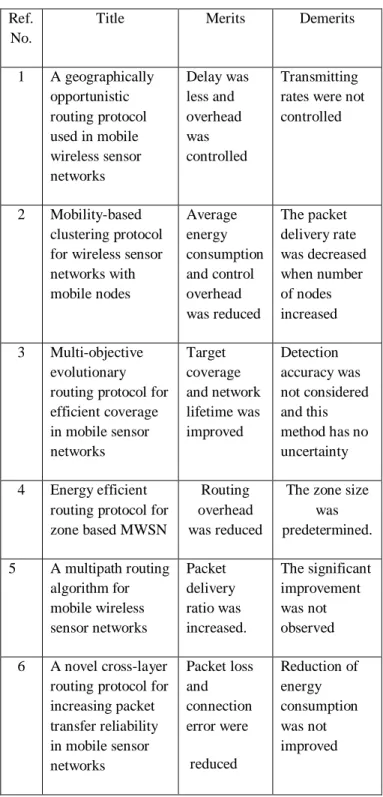
Table 3.1 Comparison of routing protocols used in WSNs Ref.
No.
Title Merits Demerits
1 A geographically opportunistic routing protocol used in mobile wireless sensor networks Delay was less and overhead was controlled Transmitting rates were not controlled
2 Mobility-based clustering protocol for wireless sensor networks with mobile nodes Average energy consumption and control overhead was reduced The packet delivery rate was decreased when number of nodes increased 3 Multi-objective evolutionary routing protocol for efficient coverage in mobile sensor networks Target coverage and network lifetime was improved Detection accuracy was not considered and this method has no uncertainty 4 Energy efficient
routing protocol for zone based MWSN
Routing overhead was reduced
The zone size was predetermined. 5 A multipath routing algorithm for mobile wireless sensor networks Packet delivery ratio was increased. The significant improvement was not observed 6 A novel cross-layer
routing protocol for increasing packet transfer reliability in mobile sensor networks Packet loss and connection error were reduced Reduction of energy consumption was not improved
7 Cluster based routing protocol for mobile nodes in wireless sensor network Data delivery rate was increased The average delay was not reduced 8 Multi-objective mobile agent-based sensor network routing using MOEA Path loss was reduced and data accuracy was improved The latency was not reduced 9 Trust opportunistic routing protocol in multi-hop wireless networks High throughput and security High routing overhead 10 Localized geographic routing to a mobile sink with guaranteed delivery in sensor networks Message cost was reduced
The QoS was not improved
11 Reliable location-aware routing protocol for mobile wireless sensor network Energy consumption was reduced End-to-end delay was not reduced 12 Location aware sensor routing protocol for MWSN Energy consumption was reduced The packet loss was high due to priority
4) COMPARISON OF LASER AND CASER
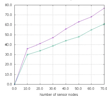
4.1) PACKET DELIVERY RATIO
Packet delivery ratio is defined as the ratio of packets that are successfully delivered to a one node compared to the number of packets that have been sent out by another node. The comparison of packet delivery ratio between proposed and existing method is shown in figure shows that Packet delivery ratio comparison between LASER and proposed CASER scheme in terms of percentage values. Packet delivery ratio means that the ratio of number of packets received divided by number of packets successfully transmitted. In this graph the number of sensor nodes are taken
from x axis and PDR in % is taken for y axis. To reduce the delay time of network the packet transmission and reception are improved so that system provides higher packet delivery ratio than the existing PDR of a network is increased.The result shows that the proposed technique.
Fig 4.1- Comparison of PDR
4.2) END-TO-END DELAY
End-to-end delay is defined as the maximum time taken by the packets to travel from one node to another node. The comparison of end-to-end delay is shown in figure.4.2.
Fig 4.2 - Comparison of End-to-End Delay
Figure 4.3shows that end to end delay comparison between LASER and proposed CASER method in terms of delay time values. In that graph we take number of sensor nodes in x axis
and delay time in y axis. The time delay is calculated as if node sends a packet to another node the time duration of difference between packets received time to packets send time. For entire network we calculate delay time in proposed system we reduce the delay time. The result shows that the proposed system provides lower delay time than the existing technique.
4.3) THROUGHPUT
It is defined as the amount of data transferred over a period of time. Its unit is kilobits per second (kpbs).
𝑇𝑟𝑜𝑢𝑔𝑝𝑢𝑡 =𝑁𝑢𝑚𝑏𝑒𝑟 𝑜𝑓 𝑝𝑎𝑐𝑘𝑒𝑡𝑠 𝑠𝑒𝑛𝑡 𝑇𝑖𝑚𝑒 𝑡𝑎𝑘𝑒𝑛 The comparison of throughput is shown in figure.6.3.
Fig 4.3- Comparison of Throughput
It shows that throughput comparison between LASER and proposed CASER scheme. The number of sensor nodes taken in x axis and in y axis throughput value is taken in bits/sec. The result shows that the proposed system provides higher throughput than the existing technique.
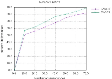
4.4) Network lifetime
The lifetime of the network is defined as the operational time of the network during which it is able to perform the dedicated task. The comparison of the network lifetime is shown in figure.4.4. Figure 4.4 shows that network lifetime comparison between LASER and proposed CASER scheme. The number of sensor nodes taken in x axis and in y axis network lifetime is taken in sec. The result shows that the proposed system provides higher network lifetime than the existing technique.
Fig 4.4- Comparison of Network Lifetime 5) CONCLUSION
There were several routing protocols developed for reliable data transmission in mobile wireless sensor networks (MWSN). In this work design a secure routing protocol suitable for large WSN to meet the market trends for high WSN penetration. A conscious aware routing protocol to increase the network performance. In that conscious score of each node we calculate by trust value, link quality, remaining energy and variation based distance metric-Mahalanobis distance. In this method is used for detecting attackers in a network by calculating trust value of each node. The attackers have lower trust value. On each sensor node, a trust repository is used to store trust information per neighbour and trust metric. Each node is characterized by its coordinates and packets are forwarded to the neighbouring node which is the closest to the destination based on geographical information. If we calculate trust value it will help for link quality of node. The link quality of a node is estimated RSSI technique. That energy take in to the account to extends the network lifetime. REFERENCES
[1] A. A. Pirzada and C. McDonald, “Trusted greedy
perimeter stateless routing,” in Proceedings of the 15th IEEE International Conference on Networks (ICON ‟07), pp. 206–211, Adelaide, Australia, November 2007.
[2] A.H. Sayed, A. Tarighat, andN. Khajehnouri,
“Network-basedwireless location: challenges faced in developing techniques for accurate wireless location information,” IEEE Signal Processing Magazine, vol. 22, no. 4, pp. 24– 40, 2005.
[3] Ahmed, U., Hussain, F „Energy efficient routing protocol
for zone based mobile sensor networks‟. Proc. Seventh Int. Wireless Communications and Mobile Computing Conf. (IWCMC), Istanbul, Turkey, July 2011, pp. 1081– 1086
[4] Aronsky, A., Segall, A.: „A multipath routing algorithm
for mobile wireless sensor networks‟. Proc. Third Joint IFIP Wireless and Mobile Networking Conf., Budapest, Hungary, October 2010, pp. 1–6
[5] Attea, B., Khalil, E., Cosar, A.: „Multi-objective evolutionary routing protocol for efficient coverage in mobile sensor networks‟, Soft Comput., 2015, 19, (10), pp. 2983–2995
[6] B. Karp and H. T. Kung, “GPSR: greedy perimeter
stateless routing for wireless networks,” in Proceedings of the Annual International Conference onMobile Computing and Networking (MobiCom ‟00), pp. 243– 254, Boston, Mass, USA, August 2000.
[7] B. Sun, L. Osborne, Y. Xiao, and S. Guizani, “Intrusion
detection techniques in mobile ad hoc and wireless sensor networks,” IEEE Wireless Communications, vol. 14, no. 5, pp. 56–63, 2007.
[8] C. Liu, K. Wu, and T. He, “Sensor localization with ring
overlapping based on comparison of received signal strength indicator,” in Proceedings of the IEEE International Conference on Mobile Ad-Hoc and Sensor Systems, pp. 516–518, October 2004.
[9] Cakici, S., Erturk, I., Atmaca, S., et al.: „A novel
cross-layer routing protocol for increasing packet transfer reliability in mobile sensor networks‟, Wirel. Pers. Commun. J., 2014, 77, (3), pp. 2235–2254
[10] D. Liu, P. Ning, and W. K. Du, “Attack-resistant locatio
estimation in sensor networks,” in Proceedings of the 4th International Symposium on Information Processing in Sensor Networks (IPSN ‟05), pp. 99–106, April 2005.
[11] Deng, S., Li, J., Shen, L.: „Mobility-based clustering
protocol for wireless sensor networks with mobile nodes‟, IET Wirel. Sens. Syst., 2011, 1, (1), pp. 39–47
[12] G. Theodorakopoulos and J. S. Baras, “On trust models
and trust evaluation metrics for ad hoc networks,” IEEE Journal on Selected Areas in Communications, vol. 24, no. 2, pp. 318–328, 2006.
[13] Han, Y., Lin, Z.: „A geographically opportunistic routing
protocol used in mobile wireless sensor networks‟. Proc. Ninth IEEE Int. Conf. Networking, Sensing and Control (ICNSC), Beijing, China, April 2012, pp. 216–221
[14] Heinzelman, W., Chandrakasan, A., Balakrishnan, H.: „Energy efficient communication protocol for wireless micro sensor networks‟. Proc. 33rd Hawaii Int. Conf. System Sciences (HICSS ‟00), Maui, USA, January 2000, p. 8020
[15] K. D. Kang, K. Liu, and N. Abu-Ghazaleh, “Securing geographic routing in wireless sensor networks,” in Proceedings of the 9th Annual NYS Cyber Security Conference: Symposium on Information Assurance, Albany, NY, USA, June 2006.
[16] K. Wu, C. Liu, J. Pan, and D. Huang, “Robust range-free
localization in wireless sensor networks,”Mobile Networks and Applications, vol. 12, no. 5-6, pp. 392–405, 2007.
[17] K.-S. Hung, K.-S. Lui, and Y.-K. Kwok, “A trust-based
geographical routing scheme in sensor networks,” in Proceedings of the IEEE Wireless Communications and Networking Conference (WCNC ‟07), pp. 3125–3129, Hong Kong, March 2007.
[18] Kim, D., Chung, Y.: „Self-organization routing protocol
supporting mobile nodes for wireless sensor network‟. Proc. First Int. Multi-Symposiums on Computer and Computational Sciences (IMSCCS „06), Hanzhou, China, June 2006, pp. 622–626
[19] Kumar, G., Vinu, M., Athithan, P., et al.: „Routing
protocol enhancement for handling node mobility in wireless sensor networks‟. Proc. IEEE Region 10 Conf. (TENCON), Hyderabad, India, November 2008, pp. 1–6
[20] L. Lazos and R. Poovendran, “SeRLoc: secure
rangeindependent localization for wireless sensor networks,” in Proceedings of the ACM Workshop on Wireless Security (WiSe ‟04), pp. 21–30, October 2004.
[21] Li, Y., Jin, D., Su, L., et al.: „Performance evaluation of routing schemes for energy-constrained delay/fault-tolerant mobile sensor networks‟, IET Wirel. Sens. Syst., 2012, 3, (3), pp. 262–271
[22] M. Garc´ıa-Otero, F. A´ lvarez-Garc´ıa, and F. J. Casaju´
s-Quiro´s, “Securing wireless sensor networks by using location information,” in Proceedings of the 16th International Conference on Systems, Signals and Image Processing (IWSSIP ‟09), June 2009.
[23] Moses, and N. S. Correal, “Locating the nodes:
cooperative localization in wireless sensor networks,” IEEE Signal Processing Magazine, vol. 22, no. 4, pp. 54– 69, 2005.
[24] N. Bulusu, J. Heidemann, and D. Estrin, “GPS-less
low-cost outdoor localization for very small devices,” IEEE Personal Communications, vol. 7, no. 5, pp. 28–34, 2000.
[25] N. Patwari, A. O. Hero III, M. Perkins, N. S. Correal, and R. J. O‟Dea, “Relative location estimation in wireless sensor networks,” IEEE Transactions on Signal Processing, vol. 51, no.8, pp. 2137–2148, 2003.
[26] N. Patwari, J. N. Ash, S. Kyperountas, A. O. Hero III, R.
L.
[27] Perkins, C., Royer, E.: „Ad-hoc on-demand distance
vector routing‟. Proc. Second IEEE Workshop on Mobile Computing Systems and Applications (WMCSA „99), New Orleans, USA, February 1999, pp. 90–100
[28] S. Ganeriwal, L. K. Balzano, and M. B. Srivastava, “Reputationbased framework for high integrity sensor networks,” ACM Transactions on Sensor Networks, vol. 4, no. 3, pp. 1–37, 2008.
[29] Soliman, H., AlOtaibi, M.: „An efficient routing approach
over mobile wireless Ad-Hoc sensor networks‟. Proc. Sixth IEEE Consumer Communications and Networkng Conf. (CCNC ‟09), Las Vegas, USA, January 2009,pp.262–271
[30] T. S. Rappaport, Wireless Communications, Principles and Practice, Prentice-Hall, Upper Saddle River, NJ, USA, 2nd edition, 2002.
[31] T.He, C. Huang, B. M. Blum, J. A. Stankovic, and T. Abdelzaher, “Range-free localization schemes for large scale sensor networks,” in Proceedings of the 9th Annual International Conference on Mobile Computing and Networking (MobiCom ‟03), pp. 81–95, September 2003.
[32] Y. Sun, Z. Han, and K. J. Ray Liu, “Defense of trust
management vulnerabilities in distributed networks,” IEEE Communications Magazine, vol. 25, no. 2, pp. 112– 119, 2008.
[33] Z. Li, W. Trappe, Y. Zhang, and B. Nath, “Robust
statistical methods for securing wireless localization in sensor networks,” in Proceedings of the 4th International Symposium on Information Processing in Sensor Networks (IPSN ‟05), pp. 91–98, April 2005.