Railway Expansion Joint Gaps and Hooks Detection Using Morphological Processing, Corner Points and Blobs

(1)

1 | P a g e

Railway Expansion Joint Gaps and Hooks

Detection Using Morphological Processing,

Corner Points and Blobs

Samiul Islam

ID: 12301053

Rubayat Ahmed Khan

ID: 11301026

Supervisor

RubelBiswas

Department of Computer Science & Engineering

April 2014

(2)

2 | P a g e

Abstract

Rail inspection is an essential task in railway maintenance. It is periodically needed for preventing dangerous situations and ensuring safety in railways. In Bangladesh it has been seen many train accidents occur due to over gapping between rail lines and also due to missing of hooks which attach the tracks to the ground. At present, this task is operated manually by a trained human operator who periodically walks along the track searching for visual anomalies. This manual inspection is lengthy, laborious and subjective.

This thesis presents a machine vision-based technique to automatically detect the presence of rail line hook and measure the gaps between each line to check whether the gap is safe or not. This inspection system uses real images acquired by a digital line scan camera installed under an automatic vehicle. Data are processed according to a combination of image processing and pattern recognition methods to achieve high performance automated detection.

The scope of this project is strictly limited to the development of a machine vision based program capable of detecting the presence of parts of interest in rail tracks, from given rail track images.

(3)

3 | P a g e

ACKNOWLEDGEMENT

Our deep thanks to our thesis supervisor Mr. RubelBiswas and to our co supervisor Mr. Md. Jahangir Alam for their generous guidance and continuous support throughout the work.

We are extremely thankful to our parents, family members and friends for their support and encouragement.

Finally we thank BRAC University for giving us the opportunity to complete our BSc. Degree in Computer Science and Engineering.

Supervised By

(4)

4 | P a g e

List of Figures

1.1 Expansion joint gaps 12

1.2 Rail line without expansion joint gaps 12

1.3 Hooks Present 13

1.4 Hook Absent 13

Chapter 1: Expansion Joint Gap Detection and Measurement

2.1 Structuring Element (Disk shaped) 21

3.1 Dilation of a binary image 24

3.2 Dilation of a Grayscale image 25

3.3 Structuring Element (Diamond shaped) 27

3.4 Structuring Element containing 25 neighbors 28

3.5 Structuring Element containing 41 neighbors 30

3.6 Flat STREL with 5 N 31

3.7 Flat STREL with 4 N 32

3.8 Flat STREL with 4 N (Sequence 3)

3.9 Dilating an image 33

3.10 Eroding an image 34

3.11 Repeated dilation of marker constrained by mask 37

3.12 Image complement 39

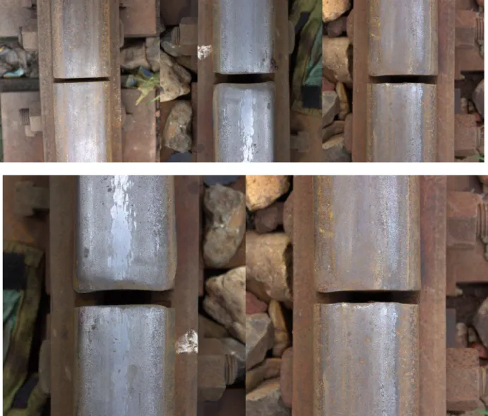
4.1 Sample Images 45

4.2 Grayscale conversion of RGB 46

4.3 Image Erosion & Reconstruction 47

4.4 Image Dilation & Reconstruction 48

4.5 Edge Detected and Enhanced 49

4.6 Enhanced portion of Interested 50

4.7 Processed Image in an Ideal Situation 51

4.8 Partitioning in terms of pixel density 52

4.9 Rail with no Expansion Gap 53

4.10 Expansion gap falls between two frames 54

(8)

8 | P a g e

Chapter 2: Rail Track Hook Detection

3 RGB Model 65 4.1 RGB Image 66 4.2 Red Channel 67 4.3 Green Channel 67 4.4 Blue Channel 68 5 Grayscale 69 6 SURF 73 7 Hook 75 8.1 Unconsidered situation 76 8.2 Unconsidered situation 76 9.1 Before Cropping 77 9.2 After Cropping 77

10 Sample of Train Images 78

11 Shi &Tomasi Points 79

12 Undetected Points 80 13 SURF Points 80 14.1 Positive Images 81 14.2 Negative Images 82 15 Matching Features 82 16 Hook Detection 83 17 Harris-Stephen Points 84 18 Undetected Points 85 19 SURF Points 86 20 Matching Features 87 21 Hook Detection 88

(9)

9 | P a g e

List of Tables

Table 1 Rules of Grayscale Dilation and Erosion 20

Table 2 Rules of padding images 26

Table 3 Sobel Operator vs. Canny Operator 41

Table 4 Result Analysis 56

Table 5 Experimental Results of Shi &Tomasi and SURF 89

Table 6 Experimental Results of Harris-Stephen and SURF 94

(10)

10 | P a g e

Abbreviation

MM - Mathematical Morphology RGB - Red Green Blue (Color Model) SE - Structuring Elements

FAST - Features from Accelerated Segment Test MSER - Maximally Stable External Regions SVM - Support Vector Machine

(11)

11 | P a g e

1.

Introduction

Railway transportation system is a very common medium of public transportation and goods or cargo shipping in North America, Europe, Australia and Asia. This popular transportation line use metallic rail tracks or lines which are fasten to the railway sleepers by using special type of metallic hooks or anchors. Railway sleepers are rectangle shaped support which helps to hold the rail lines still. These were previously wooden made and currently most of them have been replaced with pre-stressed concrete support which increase the durability and strength of the tracks. Still in many countries, we are facing railway accidents caused by collisions, derailments, fire in trains, running into obstructions etc. If we consider the situation of Bangladesh Railway, from 1998-2012 there was 4666 train accidents occur in total where 4287 were because of derailments [1]. So, almost 92% of overall accidents are caused by derailments which show its frequency is quite high. Derailment occurs due to vulnerable expansion joint gaps, missing of railway hooks, poor rail tracks etc.

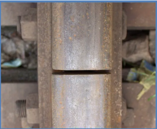
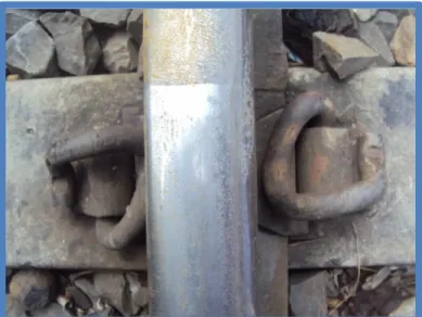
Expansion joint gaps are the gaps which are deliberately left between the rail ends to allow for expansion of the rails in hot weather. These gaps have a prefer length of 7.5mm~8mm and anything beyond this range is considered as risk. These gaps are found after each 20 m (66 feet) of rails. Railway hooks are the metallic hooks which fastens the rails with the sleepers. The conditions of these gaps, hooks and rails quality are inspected manually by a team of railway employees and engineers travelling along the track. Therefore it is very much time consuming and the quality and efficiency of work differs from person to person. In order to speed up the process, provide constant good quality and to minimize the human errors this paper aims to find a solution through software that will monitor the gaps, anchors and rail tracks quality using image processing and determine whether they are in good condition or not.

The workflow of this paper can be divided into parts. One is expansion joint gaps detection, measurement & rail lines quality check; another is railway hooks or anchors detection and security check whether those are missing or not. Approaches for these two are different in terms of processing techniques.

(12)

12 | P a g e

FIG: 1.1 Expansion joint gaps

(13)

13 | P a g e

In the first part, where the identification of expansion gaps and rail lines quality check implemented, the main techniques are used basically image segmentation, information extraction and checking and measurement. The first and most important thing of these three is image segmentation. It’s a fundamental step which is used to partition an image into separate regions and these ideally correspond to different real world objects [2]. So, basically, image segmentation is the process of partitioning a digital image into multiple segments where the goal is to simplify and/or change the representation of an image into something that is more meaningful and easier to analyze based on our specific requirements. There are many ways of image segmentation. Here we use morphological operation to segment. Before applying that, we tried many other ways of image segmentation like, Threshold based methods such as Otsu’s method, Color-based Segmentation such as K-means clustering etc. to compare and find out the best match for our work which gives us more accuracy than others. Thus we get the approach of morphological processing as it deals with the shapes of objects mainly to transform it and we can get a better view of gaps and rail lines with it. Morphological Processing is also known as mathematical morphology (MM). Such operators (like MM) consist in accordance to some proximity criterion, in selecting for each point of the analyzed image, a new grey level between two patterns (primitives) [4], [5]. Even though morphological contrast has been largely studied, there are no methodologies, from the point of view MM, capable of simultaneously normalizing and enhancing the contrast in images with poor lighting. On the other side, one of the most common techniques in image processing to enhance dark regions isthe use of nonlinear functions, such as logarithm or power functions ; otherwise, a method thatworks in the frequency domain is the homomorphism filter. However, the main disadvantage of histogram equalization is that the global properties of the image cannot be properly applied in a local context, frequently producing a poor performance in detail preservation. In a method to enhance contrast is proposed; the methodology consists in solving an optimization problem that maximizes the average local contrast of an image [3]. So, according to this explanation we can establish that, MM will work in different weather condition to provide us the expected results for this particular research. After processing the image we take as input, we get the correctly segmented output which is ready for information extraction. Once the segmentation is done successfully we applied Canny’s edge detection and Sobel edge detection. We then compare among these two outputs and choose the best one for further processing. Lastly we use another layer of MM to complete

(14)

14 | P a g e

the final extraction. Then we calculate and measure the image to know whether there is any gap or not. If there is gap present in the image, we have to calculate the length for security checking and in the mean time we do the calculation to detect damage rail lines.

FIG: 1.3 Hooks Present

FIG: 1.4 Hook Absent

We have used two techniques to detect hooks and have compared their accuracy. The steps involved in both these techniques are feature point preprocessing, detection, extraction and matching. Preprocessing is very important as it is in this stage where different types of noise are removed and the focused area is enhanced. After preprocessing came the interest point detection,

(15)

15 | P a g e

feature extraction and matching. Features of an image are pieces of information which are extracted by applying neighborhood operations. Neighborhood operations contain a square or circular neighborhood of size N with a function f and centered at p. This matrix is iterated over every pixel of the image and a value is calculated at the centre using the function f.The features we have used to detect hooks are corner points and blobs.

Corners refer to points where edges intersect. Blobs refer to regions of an image where properties like color, brightness vary within a fixed set of values. Feature detectors include BRISK, FAST, Harris-Stephen, Shi & Thomas, etc. which are used to detect corners and for detecting blobs there are MSER and SURF algorithms. In our paper we have used Harris-Stephen and Shi &Thomasi algorithms separately along with SURF, as a helper, to identify the presence or absence of anchors. Each pair of detectors (Harris-Stephen, SURF) and (Shi & Thomas, SURF) is applied over a set of sample/training images and a set of test images. Later the accuracy of identification has been compared and analyzed.

(16)

16 | P a g e

1.1 Proposed System

The purpose of our thesis is to detect rail line expansion joint gaps & anchors from static images and prepare results based on security checking. Different segmentation, feature detection algorithms mentioned above is used to detect compare the accuracy levels of the results. Images were acquired using digital camera from five locations in Dhaka city – Kamalapur Railway Station, Airport Railway Station, Khilgaon, Malibagh and Cantonment area.

As we are doing two different types of detection, we divided our work on two brunches. Both can be driven individually and independently. In the first part, our objective is to detect the expansion joint gaps and damaged lines. Then we check and formulate a result based on the given specifications. For that, we take static images as input and resize and convert it to gray-scale from RGB. The principle reason for this conversion is to reduce a 3 channel color (R = red, G = green, B = blue) to a 2 channel color (black and white). There are 256 gray levels in an 8 bit storage with the intensity of each pixel ranging from 0 – 255 [6]. On the other hand in 8 bit storage the intensity of each pixel of a RGB image is 24 bits [6]. Therefore processing a Gray-Scale image will take significantly less space and time. The second reason is image parameter of the detectors requires a Gray-Scale image. Then we segment each image using MM and pass it for information extraction. Application of edge detection algorithms and a layer of morphological operation ensure a better result image for final checking and result calculation. For the second phase, where we detect the hooks and compare the results, we select a group of images randomly for sampling and other will be preserved for testing. At first the images are cropped using a [x] window to remove stones on both horizontal sides. Here, the RGB to Gray-Scale conversion is also done for the same reason as above. The RGB images are then converted to Gray-Scale. After the conversion is done corners are detected and features are extracted from the set of sample images and stored. The third step is the detection of corners and the extractions of the features of the test images and match with the ones of the sample images. The final step is to run these steps on the same set of sample and test images using different algorithms and compare the results.

(17)

17 | P a g e

1.2 Thesis Outline

Chapter 1

Section 2 describes the previous work and basic review. Section 3 describes technical overview of image morphology and edge detection. This is followed by system design, section 4, where how we implemented ours system for detecting expansion gap is summarized. Section 5 describes the results, analysis and accuracy.

Chapter 2

Section 2 describes the previous work done on rail components. Section 3 describes grayscale and RGB images and the conversion. This is followed by technical review, section 4, where the mechanism of the algorithms we have used is described. Section describes the whole procedure, how we have detected hooks using the algorithms mentioned above. Section 6 and 7 deals with the result and comparison.

(18)

18 | P a g e

(19)

19 | P a g e

2. Background of Research

2.1 Previous Work

There are many thesis reports were published in past couple of years and many researches were conducted on different topics of railway. Mainly those were based on machine vision learning, image processing, hardware implementation and analysis to detect hooks or anchors, sleeper quality check, vegetation situation handling etc. There was no work on expansion gaps detection explicitly. So, approaching with this problem was very challenging. As rail-lines have a fixed shape and if there is a gap, surely, there will be a change in the shape. From this thought, we went through shape based different approaches of image processing and finally reached to morphological image processing. As we didn’t have any related papers, we looked through the other works to get the idea of different types of mathematical morphology. Research work of Krishan Kumar and Rajender Kumar fromShri Mata Vaishno Devi University (SMVDU), Kakryal, Katra, India was on image segmentation using MM which helps us to know about morphological operations precisely [2]. The idea of transformations using MM was studied mainly from the thesis paper documented by K. Sreedhar and B. Panlal from Department of Electronics and communication Engineering, VITS (Sreedhar) &VCE (Panlal) Karimnagar, Andhra Pradesh, India [3]. Our MM approaches were applied on Gray-Scale rather than RGB for faster calculations and speed-up processing. Theory behind this conversion is collected from the work of Professor Tarun Kumar and Karun Verma [6].

2.2 Review of Image Segmentation

This section describes some approaches of image segmentation in brief. As we are using MM or Morphological Processing, the approaches are summarized below are based on MM.

(20)

20 | P a g e

Morphology is a technique of image processing based on shapes. The value of each pixel in the output image is based on a comparison of the corresponding pixel in the input image with its neighbors. By choosing the size and shape of the neighborhood, you can construct a morphological operation that is sensitive to specific shapes in the input image.

This section describes morphological functions which can be used to perform common image processing tasks, such as contrast enhancement, noise removal, thinning, skeletonization, filling, and segmentation. Topics those are covered by this include Terminology, Dilation and Erosion, Morphological Reconstruction, Distance Transform, Watershed Segmentation, Objects, Region and Feature Measurement and Lookup Table Operations. Here, for this paper we need to know Dilation & Erosion, Structuring Elements, Dilating an Image, Eroding an Image, Morphological Reconstruction etc. brief introduction of each of these are given below.

2.2.1.1 Dilation and Erosion

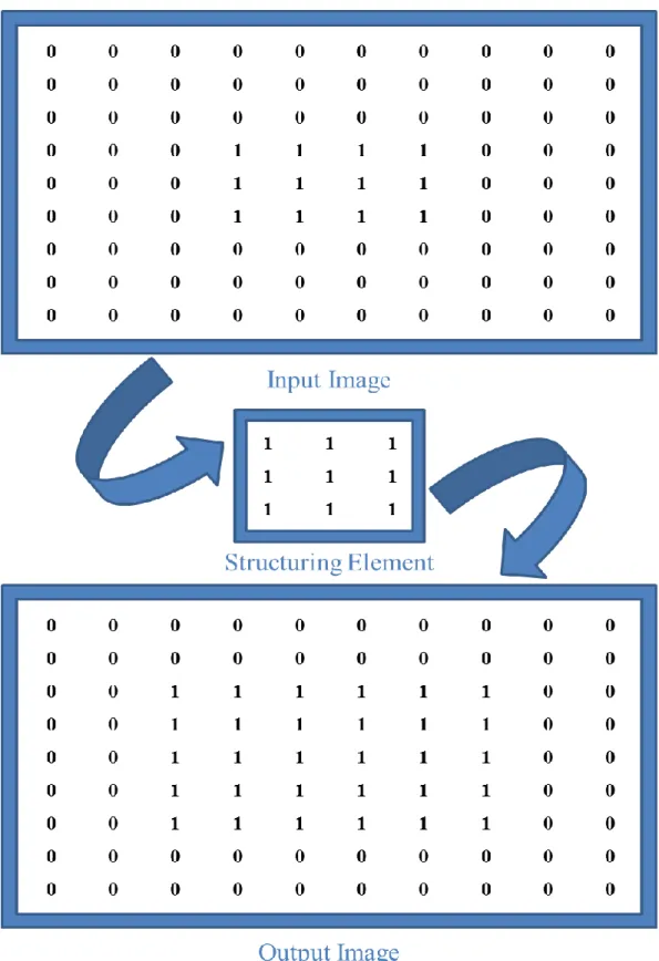
Dilation and erosion are two fundamental morphological operations. Dilation adds pixels to the boundaries of objects in an image, while erosion removes pixels on object boundaries. The number of pixels added or removed from the objects in an image depends on the size and shape of the structuring element used to process the image.

Table 1

Rules for Gray scale Dilation and Erosion

Operation Rule

Dilation The value of the output pixel is the maximum value of all the pixels in the input pixel's neighborhood. In a binary image, if any of the pixels is set to the value 1, the output pixel is set to 1.

Erosion The value of the output pixel is the minimum value of all the pixels in the input pixel's neighborhood. In a binary image, if any of the pixels is set to 0, the output pixel is set to 0.

(21)

21 | P a g e

2.2.1.2 Structuring Elements

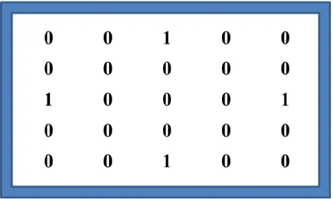
An essential part of the dilation and erosion operations is the structuring element used to probe the input image. Two-dimensional, or flat, structuring elements consist of a matrix of 0's and 1's, typically much smaller than the image being processed. The center pixel of the structuring element, called the origin, identifies the pixel of interest--the pixel being processed. The pixels in the structuring element containing 1's define the neighborhood of the structuring element. These pixels are also considered in the dilation or erosion processing. Three dimensional, or non-flat, structuring elements use 0's and 1's to define the extent of the structuring element in the x- and y-plane and add height values to define the third dimension.

FIG: 2.1 Structuring Element (Disk Shaped)

2.2.1.3 Dilating and Eroding an Image

Dilating means the application of dilation on an image using a predetermined structuring element. Eroding is same as that just the application of erosion will happen. In both cases, the input image must be in grayscale or binary or packed binary format. Without these three, any other input images will not work for such operation. Other format images must be converted to any of these three types before applying dilation and erosion.

(22)

22 | P a g e

2.2.1.4 Morphological Reconstruction

Morphological reconstruction is another major part of morphological image processing. Based on dilation, morphological reconstruction has these unique properties:

Processing is based on two images, a marker and a mask, rather than one image and a structuring element

Processing repeats until stability; i.e., the image no longer changes

Processing is based on the concept of connectivity, rather than a structuring element. Morphological reconstruction processes one image, called the marker, based on the characteristics of another image, called the mask. The high-points, or peaks, in the marker image specify where processing begins. The processing continues until the image values stop changing.

2.3 Review of Edge Detection

Edge detection is an important step in digital image processing and is mainly used in the application of feature extraction. One major application of edge detection is in the field of medical image processing. Edge detection is basically the process of detection of those regions in the image where there is an abrupt change in the brightness of the image. In this paper, we use two types of edge detection techniques; Sobel edge detector and Canny Edge Detector.

2.3.1 Sobel Edge Detector

The Sobel operator, sometimes called Sobel Filter, is used in image processing and computer vision, particularly within edge detection algorithms. It is named after Irwin Sobel, who presented the idea of an "Isotropic 3x3 Image Gradient Operator" at a talk at the Stanford Artificial Intelligence Project (SAIL) in 1968 [7]. Technically, it is a discrete differentiation operator, computing an approximation of the gradient of the image intensity function. At each point in the image, the result of the Sobel operator is either the corresponding gradient vector or the norm of this vector. The Sobel operator is based on convolving the image with a small, separable, and integer valued filter in horizontal and vertical direction and is therefore relatively inexpensive in terms of computations. On the other hand, the gradient approximation that it produces is relatively crude, in particular for high frequency variations in the image. The Kayyali operator for edge detection is another operator generated from Sobel operator.

(23)

23 | P a g e

2.3.2 Canny Edge Detector

The Canny edge detector is an edge detection operator that uses a multi-stage algorithm to detect a wide range of edges in images. It was developed by John F. Canny in 1986. Canny also produced a computational theory of edge detection explaining why the technique works.

Canny's aim was to discover the optimal edge detection algorithm. In this situation, an "optimal" edge detector means:

Good detection – the algorithm should mark as many real edges in the image as possible.

Good localization – edges marked should be as close as possible to the edge in the real image.

Minimal response – a given edge in the image should only be marked once, and where possible, image noise should not create false edges.

To satisfy these requirements Canny used the calculus of variations – a technique which finds the function which optimizes a given functional. The optimal function in Canny's detector is described by the sum of four exponential terms, but it can be approximated by the first derivative of a Gaussian.

(24)

24 | P a g e

3. Technical Review

3.1 Understanding Dilation and Erosion

In the morphological dilation and erosion operations, the state of any given pixel in the output image is determined by applying a rule to the corresponding pixel and its neighbors in the input image. The rule used to process the pixels defines the operation as a dilation or an erosion. Table 1 lists the rules for both dilation and erosion [10].

The following figure shows the dilation of a binary image. In the figure, note how the structuring element defines the neighborhood of the pixel of interest, which is circled. The dilation function applies the appropriate rule to the pixels in the neighborhood and assigns a value to the corresponding pixel in the output image. In the figure, the morphological dilation function sets the value of the output pixel to 1 because one of the elements in the neighborhood defined by the structuring element is on.

(25)

25 | P a g e

The following figure illustrates this processing for a grayscale image. The figure shows the processing of a particular pixel in the input image. Note how the function applies the rule to the input pixel's neighborhood and uses the highest value of all the pixels in the neighborhood as the value of the corresponding pixel in the output image.

FIG: 3.2 Morphological Processing (Dilation) of a Grayscale Image

3.1.1 Processing Pixels at Image Borders

Morphological functions position the origin of the structuring element, its center element, over the pixel of interest in the input image. For pixels at the edge of an image, parts of the neighborhood defined by the structuring element can extend past the border of the image [10].

To process border pixels, the morphological functions assign a value to these undefined pixels, as if the functions had padded the image with additional rows and columns. The value of these "padding" pixels varies for dilation and erosion operations. The following table details the padding rules for dilation and erosion for both binary and grayscale images.

(26)

26 | P a g e

Table 2

Rules for Padding Images

Operation Rule

Dilation Pixels beyond the image border are assigned the minimum value afforded by the data type.

For binary images, these pixels are assumed to be set to 0. For grayscale images, the minimum value for uint8 images is 0.

Erosion Pixels beyond the image border are assigned the maximum value afforded by the data type.

For binary images, these pixels are assumed to be set to 1.

For grayscale images, the maximum value for uint8 images is 255.

By using the minimum value for dilation operations and the maximum value for erosion operations, the toolbox avoids border effects, where regions near the borders of the output image do not appear to be homogeneous with the rest of the image. For example, if erosion padded with a minimum value, eroding an image would result in a black border around the edge of the output image.

3.2Structuring Elements

An essential part of the dilation and erosion operations is the structuring element used to probe the input image. Two-dimensional, or flat, structuring elements consist of a matrix of 0's and 1's, typically much smaller than the image being processed. The center pixel of the structuring element, called the origin, identifies the pixel of interest--the pixel being processed. The pixels in the structuring element containing 1's define the neighborhood of the structuring element. These pixels are also considered in the dilation or erosion processing. Three dimensional, or nonflat, structuring elements use 0's and 1's to define the extent of the structuring element in the x- and y-plane and add height values to define the third dimension [10].

(27)

27 | P a g e

3.2.1 The Origin of a Structuring Element

The morphological functions use this code to get the coordinates of the origin of structuring elements of any size and dimension.

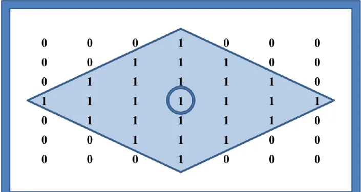
Origin = floor ((size (neighborhood) +1) /2) For example, the following illustrates a diamond-shaped structuring element.

FIG: 3.3 Structuring Element (Diamond Shaped)

3.2.2Creating a Structuring Element

According to our specific need, we create different structuring elements. The shape we want to identify, we use a SE of the same size most of the time. If our theme is to find a line from an input image, we choose an SE of line shape to detect that. There are several built-in shapes are available in MATLAB and we can use it via STREL method which will generate the SE for us. And we can also build our own SE of a particular shape [10].

(28)

28 | P a g e

We typically choose a structuring element the same size and shape as the objects we want to process in the input image. For example, to find lines in an image, we create a linear structuring element.

For example, this code creates a flat, diamond-shaped structuring element.

se = strel('diamond',3)

se =Flat STREL object containing 25 neighbors.

Decomposition: 3 STREL objects containing a total of 13 neighbors

Neighborhood:

(29)

29 | P a g e

3.2.3Structuring Element Decomposition

To enhance performance, the strel function may break structuring elements into smaller pieces, a technique known as structuring element decomposition.

For example, dilation by an 11-by-11 square structuring element can be accomplished by dilating first with a 1-by-11 structuring element, and then with an 11-by-1 structuring element. This results in a theoretical speed improvement of a factor of 5.5, although in practice the actual speed improvement is somewhat less.

Structuring element decompositions used for the 'disk' and 'ball' shapes are approximations; all other decompositions are exact. Decomposition is not used with arbitrary structuring elements, unless it is a flat structuring element whose neighborhood is all 1's.

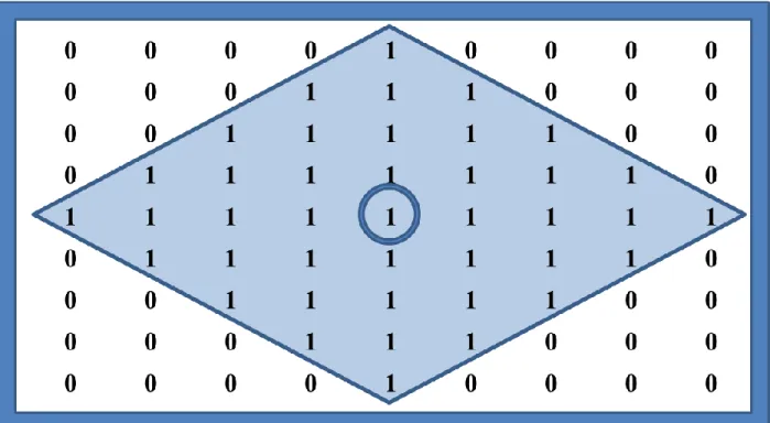
To view the sequence of structuring elements used in a decomposition, use the STREL getsequence method. The getsequence function returns an array of the structuring elements that form the decomposition. For example, here are the structuring elements created in the decomposition of a diamond shaped structuring element [10].

sel = strel('diamond',4) sel =

Flat STREL object containing 41 neighbors.

(30)

30 | P a g e

Neighborhood:

FIG: 3.5 9x9 Structuring Element containing 41 neighbors

seq = getsequence(sel) seq =

3x1 array of STREL objects

seq(1) ans =

(31)

31 | P a g e

Neighborhood:

FIG: 3.6Flat STREL object containing 5 neighbors (Sequence 1) seq (2)

ans =

Flat STREL object containing 4 neighbors.

Neighborhood:

FIG: 3.7Flat STREL object containing 4 neighbors (Sequence 2)

seq(3) ans =

(32)

32 | P a g e

Neighborhood:

(33)

33 | P a g e

3.3Dilating an Image

(34)

34 | P a g e

3.4Eroding an Image

(35)

35 | P a g e

3.5Morphological Reconstruction

Morphological reconstruction processes one image, called the marker, based on the characteristics of another image, called the mask. The high-points, or peaks, in the marker image specify where processing begins. The processing continues until the image values stop changing [10].

To illustrate morphological reconstruction, consider this simple image. It contains two primary regions, the blocks of pixels containing the value 14 and 18. The background is primarily all set to 10, with some pixels set to 11.

To morphologically reconstruct this image, perform these steps:

Create a marker image. As with the structuring element in dilation and erosion, the characteristics of the marker image determine the processing performed in morphological reconstruction. The peaks in the marker image should identify the location of objects in the mask image that you want to emphasize.

One way to create a marker image is to subtract a constant from the mask image, using imsubtract.

(36)

36 | P a g e

marker = imsubtract(A,2) marker =

Call the imreconstruct function to morphologically reconstruct the image. In the output image, note how all the intensity fluctuations except the intensity peak have been removed.

(37)

37 | P a g e

3.5.1

Understanding Morphological Reconstruction

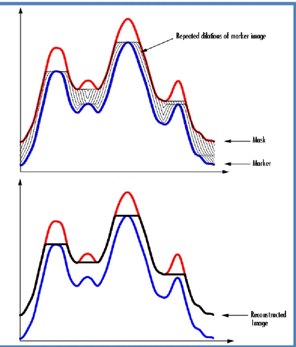
Morphological reconstruction can be thought of conceptually as repeated dilations of the marker image until the contour of the marker image fits under the mask image. In this way, the peaks in the marker image "spread out", or dilate.

This figure illustrates this processing in 1-D. Each successive dilation is constrained to lie underneath the mask. When further dilation ceases to change the image, processing stops. The final dilation is the reconstructed image. The figure shows the successive dilations of the marker.

(38)

38 | P a g e

3.6Image Complement

Image complement is basically applying a negation on an image. Negation is an operation on one

FIG: 3.12 Image Complement

FIG: 3.12 (a) Original Image

FIG: 3.12 (b) Binary Image

(39)

39 | P a g e

logical value, typically the value of a proposition that produces a value of true when its operand is false and a value of false when its operand is true [9].

New complemented image will consume the same size of the input image. In the complement of a binary image, zeros become ones and ones become zeros; black and white are reversed. In the complement of an intensity or RGB image, each pixel value is subtracted from the maximum pixel value supported by the class (or 1.0 for double-precision images) and the difference is used as the pixel value in the output image. In the output image, dark areas become lighter and light areas become darker.

3.7Understanding Sobel Edge Detector

Sobel is the well-known simple conventional edge detection technique in which 3x3 convolution masks are used for detection of the edges in x and y directions. These two 3×3 kernels which are convolved with the original image to calculate approximations of the derivatives - one for horizontal changes, and one for vertical [11]. If we define A as the source image, and Gx and Gy are two images which at each point contain the horizontal and vertical derivative approximations, the computations are as follows:

Where * here denotes the 2-dimensional convolution operation.

Since the Sobel kernels can be decomposed as the products of an averaging and a differentiation kernel, they compute the gradient with smoothing. For example,

G

xcan be written as

(40)

40 | P a g e

3.8 Understanding Canny Edge Detector

Canny is another well-known conventional edge detection algorithm which is popular due to its optimum performance. It is basically an optimization problem with constraints. Three different criteria are addressed in this detector i.e. localization, low error rate and single response to the single edge. These parameters were implemented by using the canny operator [11].

5.1 Steps in Canny Edge Detector:-

5.1.1 Convert to Gray scale: - First convert the image to gray scale using some type of RGB to gray scale conversion.

5.1.2 Noise Reduction: - Noise reduction implies some sort of blurring operations. Gaussian filter is usually used to reduce noise. Commonly used filter is 5 × 5 filter.

5.1.3 Compute Gradient Magnitude and Angle: - The derivatives (Dx(x, y) and Dy(x, y)) of the image in both x and y directions are calculated. Then the angle of the gradient and the gradient magnitude are also calculated. The angle of gradient is computed as follows:-

𝜃 = 𝑎𝑟𝑐𝑡𝑎𝑛

𝐷𝑥(𝑥, 𝑦)

𝐷𝑦(𝑥, 𝑦)

5.1.4 Non-Maximum Suppression: - The “non-maximal suppression” keeps only those pixels on an edge which have the maximum gradient magnitude. The maximal magnitudes should always occur right at the edge boundary, and then the gradient magnitude should always fall off with distance from the edge.

So, three pixels in a 3 × 3 around pixel (x, y) are examined:

If θ(x, y) = 0◦, then the pixels (x + 1, y), (x, y), and (x − 1, y) are to be considered. If θ(x, y) = 90, then the pixels (x, y + 1), (x, y), and (x, y − 1) are to be considered.

If θ(x, y) = 45◦, then the pixels (x + 1, y + 1), (x, y), and (x − 1, y − 1) are to be considered.

If θ(x, y) = 135◦, then the pixels (x + 1, y − 1), (x, y), and (x − 1, y + 1) are to be considered.

If pixel (x, y) has the highest gradient magnitude out of all the three pixels which are considered, it is kept as an edge. If one of the other two pixels has a higher gradient magnitude, then pixel (x, y) is not on the “center” of the edge, thus, should not be considered as an edge pixel.

(41)

41 | P a g e

Table 3

Sobel Operator Vs. Canny Operator

Operator Advantages Disadvantages

Classical operators like Sobel operator

Simplicity Inaccurate, sensitive to

noise Gaussian operators

like Canny

Improved signal to noise ratio, Shows better detection in the noise conditions

Complex computations, Takes more time.

(42)

42 | P a g e

3.9 Technical View of Expansion Gap

For single rail fish-plated track, the width of expansion gaps depends on the length of the separate rail, temperature at the time of linking the track and the maximum annual rail temperature. The expansion gap should correspond to the linking temperature. If the gap is less than required, the track may buckle in hot weather. Contrariwise, if the gap is more than required, the rail ends may get damaged. Expansion gaps are kept in such a way that even at maximum rail temperature the rail ends have a gap of 1 mm [8]. Expansion gaps at other temperatures are calculated by the formula as follows:

e = L a t * 10^3

e = expansion in mm

L = length of the rail in m (say 20m)

a = coefficient of expansion of rail steel, which is equal to 0.00001152 per degree centigrade t= change in temperature in centigrade.

Assuming a maximum rail temperature of 70oC, the expansion gap at 40oC will be:

= 1mm + (70-40) * 0.00001152 *20 * 10^3 = 1mm +6.912

(43)

43 | P a g e

4. System Design

4.1 Tools, algorithms and methodology

Tools we used are MATLAB R2013a and Image Processing Toolbox Algorithms we used are Sobel Edge Detection, Canny Edge Detection etc.

Methodology we followed are image dilation, image erosion, morphological reconstruction, image complements, a custom partitioning system for efficient information extraction and risk calculation etc.

(44)

44 | P a g e

(45)

45 | P a g e

4.3 Data Collection

In the field of image processing, data collection is the most crucial part because if the images are not precise & accurate, we will not get expected output. In our paper, the sample images are collected from different parts of Dhaka city to compare the result and to ensure of building such a method which will work on any parts of Bangladesh. We do consider different weather situation and images we collected was from different times through-out the day. We resized those images to a lower matrix for faster processing without risking image details those are needed for ensuring a correct output. There are few sample images are shown below:

(46)

46 | P a g e

4.4 Morphological Processing of Input Image

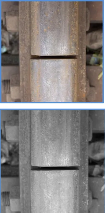
In our workflow, first of all we convert the acquired RGB input image to grayscale image for a better and faster processing as we do not use color based segmentation for our information gathering.

(47)

47 | P a g e

After that, we process that image through several processing techniques of image morphology. We use image erosion on the grayscale image to identify the lowest pixels as the gap is most of the time contains black (close to zero in grayscale) region. Those black regions we obtain can be an actual gap or noises. To refine it more precisely, we reconstruct our raw grayscale using the erosion output which ensures the darken regions in the output.

(a)

(b)

(48)

48 | P a g e

Now we have an image where the black regions are marked and if there is gap it will fall in that region. Problem is, for human eyes this is quite fine to detect the gap from this step but, if we run edge detection or pixel value calculation to know the exact position, width, length of the expansion gap, we need to filter it in a more concise manner. To do that, we are using image dilation which will create an image with the highest pixel values from its neighbors.

(a) (b)

(c) (d)

FIG: 4.4 (a) Image Dilation, (b) Complement of dilated image (c) Complement of previous reconstruction (d) Reconstruct from b & c

(49)

49 | P a g e

As we have the second phase of reconstruction which is more categorized to emphasize the gap, we are applying edge detection now to take the information out the image. We are using mainly sobel which is fast in terms of processing but sensitive to noise. As long as we are having decent results using a simple method, we need not to go for complex processing. After the edge detection, we ran a simple dilation with line structuring elements to emphasize each pixel more and actually this dilated image has the more positive (value with 1 in a binary image) pixels corresponding to the input ensures us an efficient calculation of gap. As our camera height and view is strictly fixed in a certain position, we can eliminate portions in which there is no rail. So, ultimate image will be like below:

(50)

50 | P a g e

FIG: 4.6 Enhanced portion of interest

This is our final processed part before calculating the presence of gap, width and security checking procedure.

(51)

51 | P a g e

4.5 Identifying Partitions and Checking

Soon we are finished with morphology and edge detection; we will have images ready like 4.6. We implemented a partition system for further processing to identify and measure the length of the gap. For an ideal scenario, we will have an image as posted as in below:

FIG: 4.7 Processed image in the ideal situation

This image shows how a line with a certain gap will look like after the morphological processing.

(52)

52 | P a g e

FIG: 4.8 Partitioned image in terms of pixel frequency

Here is the detailed processed image with their pixel frequency in each region. We have broken the image (with gap) into 5 parts where the each part has a definite pixel frequency for each of their rows. Pixel frequency of (180-210) indicates that it is a starting of a gap and from that line or row we are counting the length of the gap until we reach to a portion which have the same pixel frequency as before denotes the end of the gap.

It is obvious that, in each frame there will not be each of these 5 regions. Suppose, if we have an image with a continuous line and no expansion gap, then our program should be in the region 1 for the entire checking period of that frame. That is why, we are also checking whether the finds the starting condition or not. If not, we are recording this as a NO GAP DETECTED frame.

(53)

53 | P a g e

FIG: 4.9 Rail with no expansion gap

It is also not ensured that, each time we will get a frame (image) in which the expansion gap will be somewhere in the middle. It might be at the end or beginning of a frame and it might be partially captured. Any calculation based on a single frame at that time might produce misleading information as the actual gap length is now distributed in two distinguish frame. It will be a common scenario when we will start the phase 2 of our project for real time computation. To overcome this issue, we introduce a global variable accessible for each frame which will keep the value of the gap from previous frame. If there is no gap or a gap which ended successfully in the previous frame, the value of the variable will be set to zero. It will contain the gap value only if there is an unfinished gap in the previous frame. In that case, the gap value of the current frame will be added to the previous value for the entire length of gap.

(54)

54 | P a g e

(55)

55 | P a g e

FIG: 4.11 Frame rate issue

PrevGapVal – Value of a gap which is not ended of an immediate previous frame; otherwise 0 CurrGapVal – Value of gap in a current frame which is started right after a frame with PrevGapVal

So,

(56)

56 | P a g e

5. Experiment and result analysis

The experimental results are shown in the table 4 below:

Image Gap Presents Situations ExperimentalResult

1. T Normal Daylight 2. T Sunny 3. F Normal Daylight 4. F Sunny 5. T Normal Daylight 6. T Normal Daylight 7. T Sunny 8. T Sunny 9. T Sunny 10. T Low Light 11. T Normal Daylight 12. T Normal Daylight 13. F Low Light 14. T Low Light 15. T Low Light 16. T Low Light 17. T Low Light 18. T Normal Daylight 19. T Normal Daylight 20. T Normal Daylight 21. T Low Light

(57)

57 | P a g e 22 T Low Light 23 T Low Light 24 T Normal Daylight 25 T Sunny 26 F Normal Daylight 27 F Sunny 28 T Normal Daylight 29 T Normal Daylight 30 T Sunny 31 T Sunny 32 T Sunny 33 T Low Light 34 T Normal Daylight 35 T Normal Daylight 36 F Low Light 37 T Low Light 38 T Low Light 39 T Low Light 40 T Low Light 41 T Normal Daylight 42 T Normal Daylight 43 T Normal Daylight 44 T Low Light 45 T Low Light 46 T Low Light

(58)

58 | P a g e 47 T Normal Daylight 48 T Low Light 49 T Low Light 50 T Normal Daylight 51 T Sunny 52 T Sunny 53 T Sunny 54 T Normal Daylight 55 T Normal Daylight 56 T Normal Daylight 57 T Sunny 58 T Sunny 59 T Sunny 60 T Low Light 61 T Normal Daylight 62 T Normal Daylight 63 F Low Light 64 T Low Light 65 T Low Light 66 T Low Light 67 T Low Light 68 T Normal Daylight 69 T Normal Daylight 70 T Normal Daylight 71 T Normal Daylight

(59)

59 | P a g e 72 T Sunny 73 T Sunny 74 T Sunny 75 T Low Light 76 T Normal Daylight 77 T Normal Daylight 78 F Low Light 79 T Low Light 80 T Low Light 81 T Low Light 82 T Low Light 83 T Normal Daylight 84 T Normal Daylight 85 T Normal Daylight 86 T Normal Daylight 87 T Sunny 88 T Sunny 89 T Sunny 90 T Low Light 91 T Normal Daylight 92 F Normal Daylight 93 T Sunny 94 F Sunny 95 T Normal Daylight

(60)

60 | P a g e 96 T Normal Daylight 97 T Normal Daylight 98 T Sunny 99 T Sunny 100 T Sunny

5.1 Accuracy Calculation

Table 5

Test Image Classification based on Presence of Gap

Image Type Test Image Correct Output

Image with expansion gap 90 79

Image with expansion gap 10 10

Total Image 100 89

Table 6

Test Image Classification based on light

Image Type Test Image Correct Output

Sunny 27 22

Low Light 33 30

Normal Daylight 40 37

(61)

61 | P a g e

Image with expansion gap:

𝐶𝑜𝑟𝑟𝑒𝑐𝑡 𝑂𝑢𝑡𝑝𝑢𝑡

𝑇𝑒𝑠𝑡 𝐼𝑚𝑎𝑔𝑒 ×100%

=79

90 x 100%

= 87.78%

Image without expansion gap:

𝐶𝑜𝑟𝑟𝑒𝑐𝑡 𝑂𝑢𝑡𝑝𝑢𝑡 𝑇𝑒𝑠𝑡 𝐼𝑚𝑎𝑔𝑒 ×100% =10 10 x 100% = 100% Sunny condition: 𝐶𝑜𝑟𝑟𝑒𝑐𝑡 𝑂𝑢𝑡𝑝𝑢𝑡 𝑇𝑒𝑠𝑡 𝐼𝑚𝑎𝑔𝑒 ×100% =22 27 x 100% = 81.48%

(62)

62 | P a g e

Low Light Condition:

𝐶𝑜𝑟𝑟𝑒𝑐𝑡 𝑂𝑢𝑡𝑝𝑢𝑡

𝑇𝑒𝑠𝑡 𝐼𝑚𝑎𝑔𝑒 ×100%

=30

33 x 100%

= 90.91%

Normal Daylight Condition:

𝐶𝑜𝑟𝑟𝑒𝑐𝑡 𝑂𝑢𝑡𝑝𝑢𝑡 𝑇𝑒𝑠𝑡 𝐼𝑚𝑎𝑔𝑒 ×100% =37 40 x 100% = 92.50% Overall accuracy: 𝐶𝑜𝑟𝑟𝑒𝑐𝑡 𝑂𝑢𝑡𝑝𝑢𝑡 𝑇𝑒𝑠𝑡 𝐼𝑚𝑎𝑔𝑒 ×100% = 89 100 x 100% = 89.00%

(63)

(64)

64 | P a g e

(65)

65 | P a g e

2. Previous Work

Many machine vision techniques have been developed which deal with railway components but not many are there that focus directly on hooks. The paper from the IBM T.J. Watson Research Centre [20], worked on railway components like anchors/hooks, plates, etc. It has detected hooks based on Adaboostclassifier. Multiple classifierswere run simultaneously but the detection results were selected based on one classifier which had the highest detection in the last 50 frames. 50 was the threshold used in this paper.

Paper [21] by YohannRubinsztejn, University of Manchester, proposed to detect rail anchors by using Viola-Jones object detection framework. This framework uses integral image technique to compute the Haar Wavelet features, used Adaboost as the learning algorithm and lastly it uses a cascade of classifiers. A set of positive and negative images were used to construct the dataset. Then a set of feature template was built from it. The training set along with the feature template was fed to Adaboost. This was how the detector was created. Then it was applied on rail images to detect true and false instances of anchors.

Paper [23] also worked on a number of railway components and detection of hooks was a part. In this paper correlation was used. Although correlation is neither scale nor orientation invariant it could be applied using filters at multiple orientation and scales and then merging the correlation results. Of many correlation techniques Optimal Tradeoff Maximum Average Correlation Height (OT – MACH) technique was used. A set of images were collected and categorized into classes and were then trained using the algorithm. This method was used for detecting grounded hooks. In order to find the missing ones two approaches were taken. Firstly the OT_MACH algorithm itself but it was not very accurate and secondly by measuring the average interval and deviation between anchors. When anchors were detected the gap was smaller than the gap which arose due to the presence of a missing anchor.

In our paper we are proposing to detect anchors using feature detection algorithms combined with a blob detection algorithm. We believe that using features would be a simpler technique rather than using different kinds of classifiers and trainig algorithms. The algorithms we have used are scale and orientation invariant. Moreover we are showing a quantitative analysis of accuracy of the different algorithms we have used.

(66)

66 | P a g e

3. RGB vs.Grayscale Overview

3.1.1 RGB Color Model

The RGB color model is color model where red (R), green (G) and blue (B) colors are merged together to produce a range of colors. As 3 colors define the RGB model, the geometric representation is a three dimensional cube. Each node of the cube represents a particular color. Each color has three components – red, green and blue and each component ranges from 0 – 1. Therefore any color is represented by R, G or B where the presence of a component is denoted by 1 and the absence is denoted by 0. White is represented by (1, 1, 1) whereas black is represented by (0, 0, 0).

Figure 3: RGB Color Model

3.1.2 RGB Images

RGB images consist of three channels and they are red (R), green (G) and blue (B). In a 24-bit image each channel contains 8 bits. The whole RGB image is composed of three images one for each channel. Each image stores pixel with brightness ranging from 0 to 255. The figure

(67)

67 | P a g e

4.1shows RGB image with all the 3 components present, figure 4.2only has the red channel on, figure 4.3 and figure 4.4 show green channel and blue channel respectively.

Figure 4.1 RGB Image

(68)

68 | P a g e

Figure 4.3 Green Channel

(69)

69 | P a g e

3.2 Grayscale Images

Grayscale images are images whose pixels carry only the intensity information. It does not carry any color component. The intensity ranges from black (darkest) to white (brightest). Grayscale images are also called monochromatic. The intensity information is represented in 3 ways.

1. Total black is represented by 0 and white is represented by 1. The different intensity gray colors between them are represented as fractions.

2. Percentage representations where 0% denotes black and 100% denotes white. The colors between then are denoted by integers in percentage.

3. Pixel depth representation. For an 8 bit per pixel image 0 is black and 255 is white and for a 16 bit per pixel image 0 is black and 65535 is white.

Figure 5 Grayscale Image

3.3RGB to Grayscale Conversion

The main reason for this conversion is to reduce space and processing time. RGB consists of three channels whereas grayscale consists for one. The conversion is done by calculating the weighted sum in a linear RGB space.

The linear Y is calculated by .2989 R + .5870 G + .1140 B in MATLAB, the toolbox we have used in our work.

(70)

70 | P a g e

4. Technical Review

4. 1 Overview of Harris Stephen

The Harris Stephen algorithm was developed to recognize image sequences from a moving camera by extracting and tracking image features. Matching images using just edges work when the camera is still but when it comes to a camera in motion just edges are not enough. The algorithm was developed based on two image sequences which contained corners and edges. Edge matching worked poor due to difference in fragmentation in sequences. Therefore the solution was to detect both corners and edges from an image. To detect corners the Moravec’s corner detector was modified.

Moravec’s corner detector operates by using a local window in the image. The window shifts by small amount in various directions and calculate the average change in the intensity. Moravec’s algorithm has the following cases:

i) If the intensity of the image within the window is consistent then the shifts will result in small change.

ii) If the window finds and edge, moving the window along it will bring a small change and moving it perpendicular will bring a large change.

iii) If the windowed image is a corner or an isolated point, then every shift will result in a large change. Thus a corner can be detected when the change is large.

This is the mathematical representation

Ex,y= 𝑢.𝑣wu,v | Ix+u, y+v– Iu,v|2

Where w is the image window, (x,y) are the shifts. The Moravec’s detector has the following drawbacks.

i) Due to the discrete number of shifts at every 45 degrees the response is anisotropic. ii) As the window is rectangular and binary, the response in noisy.

iii) The detector responds edges more as the minimum of E is taken into account. The Harris Stephens algorithm solves this problem.

(71)

71 | P a g e

i) Through performing analytical expansion about the shift origin all possible shifts can be covered.

ii) Using a Gaussian circular window can reduce noise

iii) Reformulating the corner measure can avoid the edge response Based on the third solution, the change E, can be written as,

E(x,y) = (x,y) M (x,y)T

Where M is a 2x2 symmetric matrix.

M = 𝐴 𝐶 𝐶 𝐵

If α and β are the Eigen values of M then they will be proportional to the principal curvatures of the local autocorrelation function [13]. The following cases can be drawn.

i) If both α and β are small then the images within the window is of consistent intensity. ii) If α is high β is low, it indicates an edge.

iii) If α and β are high it indicates a corner.

The measure of the corner and the edge, the response, was used to select isolated corner pixels. The corner response is indicated by,

R = Det – kTr2

WhereDet = αβ and Tr = α + β. R is positive in corner detection and negative in edge detection. A corner is detected if the corner region pixel is an eight way local maxima. An edge detected if the response of an edge pixel is negative and local minima in either x or y direction.

4.2 Overview of Shi &Tomasi (Minimum Eigen)

Shi and Tomasi detector detects corner points by measuring the feature dissimilarity between the first frame and the current frame in a motion. The idea of the algorithm is when the divergence of the features of the two frames is very large they are abandoned. The paper [24] proved that pure translation is not adequate but linear warping and translations are. This algorithm also detects features which are best for tracking.

(72)

72 | P a g e

When a camera moves, the points in an image change in a very complex way. The amount of motion is called the displacement at a point X(x,y). X is any point in an image with the coordinates x and y. The displacement vector is represented in the following way

 = DX + d where D is the deformation matrix represented by

D = 𝑑𝑥𝑥 𝑑𝑥𝑦 _𝑑𝑦𝑥 _𝑑𝑦𝑦

d is the translation of the feature window’s centre. Xmeasured with respect to the window’s centre. During motion a point Xin the image I gets into a new point AX+ d in a new image J where is 1 + D:

I(X) = J (AX+ d)

Given two images I and J and a window size in I, tracking is finding out the 6 parametres in D. Although small window size is preferred but a small window size means tracking is harder as the changes noticed will be very less. While tracking the deformation matrix D is likely to be small so therefore it is safe to set D to the zero matrix. Regardess of the methods used for tracking every information of an image is not contained in all parts of an image. In order to solve this problem researchers have proposed to track corners or windows with a high spatial frequency content. But the problem with these points are they are based on an uninformed idea hence they are not assured to be the best for tracking.

Z is a symmetric matrix derived while computing image motion in [24].

Z = _gxgyg2x gxgy_g2x

If both eigen values of Z is large it can represent a corner. If both eigen values are small it means a coarse intensity profile within a window and one small and one large value means an undirectional texture pattern.

(73)

73 | P a g e

A feature with a high texture can be a bad feature. For exmaple, a scenarion in an image might appear in such a way that shows an edge but in not in reality. The measure of the dissimilarity by this algorithm will identify this issue.

4.3 Overview of SURF (Speeded Up Robust Features)

SURF is a scale and rotation invariant detector and descriptor. It is in fact a robust and a distinct detector. In order to be rotation invariant it identifies a reproducible orientation for the interest points. This is done by calculating Haar Wavelet responses in the x and y direction, which is a circular neighborhood with a radius of 6s around the interest point. S is the scale at which the interest point is detected [25]. Six calculation are required to calculate the Haar response in the x or y direction.

After the responses are calculated they are weighted with a Gaussian filter of  = 2.5s. The responses are arranges as vectors. The orientation window covers an angle of𝜋₃. The horizontal and vertical responses within the window are added and a new vector is created. The longest vector provides its orientation to the interest point.

In order to extract the descriptor the first step is to build a square region of size 20s around the point of interest. The square window is subdivided into 4x4 squares. For each sub region simple features are detected. dx = Haar wavelet response in horizontal direction and dy = Haar wavelet response in vertical direction. The dx and dy are weighted with Gaussian filter of  = 3.3s centered at the interest point. The responses dx and dy are added up over each sub region. The absolute values dx and dy are also added to extract information about the polarity of the intensity images. Therefore each sub region has a 4 dimensional descriptor v

v = (Σdx, Σdy, Σ dx , Σ dy )

Figure 6 shows the properties of the descriptor from three different intensity structures within a sub region.

(74)

74 | P a g e

Figure 6

The first square is a homogeneous region and its corresponding values are low. The second square is a region with an increasing frequency in the x direction. As a result it has a high Σ dx . The last square is a region where the intensity is increasing in the x direction and its Σdx and Σ dx values are high.

(75)

75 | P a g e

5. System Design

5.1 Tools

To build the proposed system we have used MATLAB R2013A.

Algorithms used are Shi and Tomasi corner detector, Harris-Stephen corner detector and SURF blob detector. 5.2 Methodology Yes No RGB images acquired Preprocessing Conversion to grayscale RGB images acquired

Training set Test set

Corner points and blobs detected Corner points and blobs detected

Training set

If

matches>threshold

Hook missing Hook detected

(76)

76 | P a g e

5.3 Data Collection

For this very experiment we could not find any universal image set. Therefore we had to go to the rail tracks physically and collect the images. The pictures were taken with a twelve mega pixel digital camera. In the papers we have studied so far related to rail way components [20], [21] and [22], all have used a vehicle with cameras mounted on it that ran on the rail line to take the images. As this paper is only concerned with detection and comparison of accuracy levels of two algorithms, we have saved the vehicle factor for future work which will be discussed in section 6. Hence we have taken the images manually holding the camera at a height of one and a half feet (approximately) perpendicular to the hooks. One and a half feet is a decent height. This is because increasing it would make the object of interest move further away plus noise like stones would be more visible in the image frame. Lower than one and a half feet would bring the object closer but as we are using a regular digital camera blurring became an issue.

For this paper we have only considered totally visible hook plates and the lighting condition was daylight as shown in Figure 7.

Figure 7

In the rail tracks we have discovered many scenarios where the hooks are completely or partially covered by stone layers or other objects. The following figures show such scenarios. We will not be dealing with such situation in this paper.

(77)

77 | P a g e

Figure 8.1

Figure 8.2

(78)

78 | P a g e

We have taken pictures from three different locations in Dhaka city and they are Khilgaon, Malibagh and Cantonment. After the images were acquired the first step of the experiment was preprocessing.

5.4 Pre Processing

In the preprocessing phase every image obtained were resized to 200 x 200 pixels. Reducing the image size to 200 x 200 decreases processing time and space. Then they were cropped by a window of 197 x 62. The reason behind the cropping was to reduce the stone noise which was visible in the image frame. The following diagram shows the image before and after cropping.

Figure 9.1 Before Cropping

(79)

79 | P a g e

5.5 Detection of Hooks Using Shi &Tomasi Minimum Eigen Detector and SURF Detector

After preprocessing all the images taken were divided into 2 sets – (i) training images and (ii) test images. Images for training and testing have been chosen randomly. The following dropbox links will lead you to the train and test images respectively. Two hundred images were chosen for training and one hundred images were used for testing.

Figure 10 Samples of training images (after prepro