Intelligence in 5G networks

Academic year 2018-2019 (796 )

Department of Information Engineering (DEI) Doctoral thesis in Information Engineering

Intelligence in 5G networks

Over the past decade, Artificial Intelligence (AI) has become an important part of our daily lives; however, its application to communication networks has been partial and unsystematic, with uncoordinated efforts that often conflict with each other. Providing a framework to integrate the existing studies and to actually build an intelligent network is a top research priority. In fact, one of the objectives of 5G is to manage all communications under a single overarching paradigm, and the staggering complexity of this task is beyond the scope of human-designed algorithms and control systems.

This thesis presents an overview of all the necessary components to inte-grate intelligence in this complex environment, with a user-centric perspec-tive: network optimization should always have the end goal of improving the experience of the user. Each step is described with the aid of one or more case studies, involving various network functions and elements.

Starting from perception and prediction of the surrounding environment, the first core requirements of an intelligent system, this work gradually builds its way up to showing examples of fully autonomous network agents which learn from experience without any human intervention or pre-defined behav-ior, discussing the possible application of each aspect of intelligence in future networks.

1 Introduction 5

2 A review of machine learning techniques 9

2.1 Prediction techniques . . . 10

2.1.1 Graphical Bayesian models . . . 10

2.1.2 Support Vector Machines . . . 12

2.1.3 Linear regression techniques . . . 14

2.1.4 Random Forest and k-Nearest Neighbors . . . 15

2.1.5 Neural Networks . . . 15

2.1.6 Kalman filters . . . 17

2.2 Reinforcement Learning . . . 19

2.2.1 Markov Decision Processes . . . 21

2.2.2 Q-learning . . . 22

2.2.3 Deep Q-learning . . . 25

3 Prediction and anticipatory networking 29 3.1 Predicting the wireless channel . . . 30

3.1.1 State of the art . . . 30

3.1.2 Studied scenario . . . 32

3.1.3 Learning parameters and results . . . 34

3.2 Predicting battery usage in smartphones . . . 38

3.2.1 State of the art . . . 39

3.2.2 Data analysis . . . 40

3.2.3 Results . . . 45

3.3.3 Parameter optimization and results . . . 54

4 A predictive approach to providing Quality of Service 59 4.1 State of the art . . . 63

4.1.1 Single-path latency-minimization protocols . . . 63

4.1.2 Multi-path aggregation protocols . . . 66

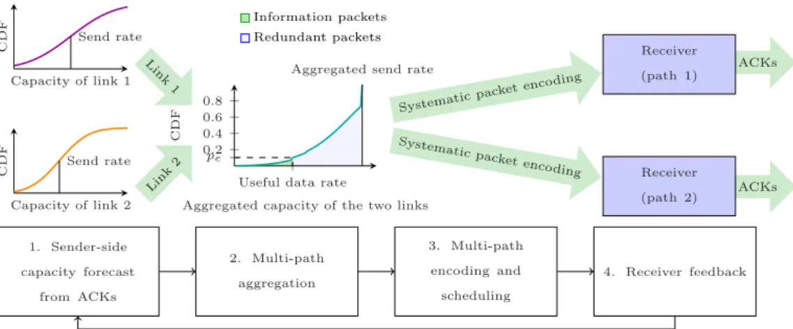
4.2 The LEAP protocol . . . 67

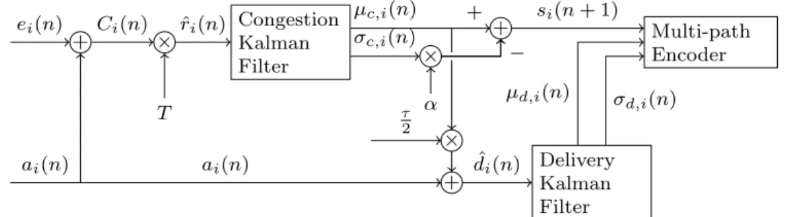
4.2.1 Congestion control on a single path . . . 70

4.2.2 Integrating single-path congestion control and multi-path coding . . . 74

4.2.3 Aggregating flows through coding . . . 75

4.2.4 Scheduling and retransmission . . . 77

4.2.5 Computation of the combined capacity in the two-path Gaussian case . . . 78

4.2.6 Implementation considerations . . . 82

4.3 Experimental results . . . 83

4.3.1 Combining the traces . . . 84

4.3.2 Single-path congestion control . . . 84

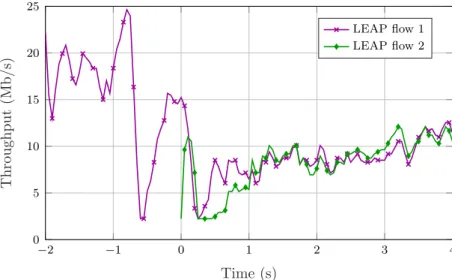
4.3.3 Combining multiple paths . . . 90

5 Providing Quality of Experience guarantees with Reinforce-ment Learning 95 5.1 State of the art . . . 97

5.1.1 Reinforcement Learning and DASH . . . 100

5.2 System model . . . 101

5.2.1 Video streaming model . . . 101

5.2.2 Reward function . . . 103

5.2.3 Defining the Markov Decision Process . . . 104

5.3 Deep Q-learning for DASH adaptation . . . 105

5.4 Simulation and results . . . 107

5.4.4 Summary of performance . . . 122

6 Optimizing Smart City services with data-driven techniques125 6.1 Bike sharing in Smart Cities . . . 127

6.2 State of the art . . . 130

6.2.1 Rebalancing bike sharing systems . . . 131

6.2.2 User incentives and pricing . . . 133

6.3 System model . . . 135

6.3.1 The bike sharing system as a network . . . 135

6.3.2 Downtime at a station . . . 137

6.3.3 Expected number of system failures . . . 140

6.3.4 The incentive problem . . . 140

6.3.5 The incentive model . . . 141

6.3.6 Solving the incentive problem . . . 144

6.4 Dynamic rebalancing . . . 147

6.4.1 Preliminaries . . . 148

6.4.2 System-wide rebalancing problem . . . 149

6.4.3 Single-vehicle optimization . . . 151

6.4.4 Multi-vehicle optimization . . . 154

6.4.5 Simulation settings and analysis . . . 155

6.5 Results . . . 160

6.5.1 Performance . . . 160

6.5.2 Rebalancing effort . . . 162

6.5.3 Cost analysis . . . 163

7 Exploiting Smart City data to optimize the network 167 7.1 Smart Cities and networks . . . 168

7.2 The SymbioCity concept . . . 170

7.3 Analyzing traffic data . . . 175

7.4 State of the art . . . 178

7.6 Adaptive vMME Allocation . . . 188 8 Conclusion 195 8.1 Published works . . . 196 Bibliography 199 List of Acronyms 221 Acknowledgments 227

Introduction

Although Artificial Intelligence (AI) is already an important part of our daily lives, seamlessly performing tasks such as speech processing and image recog-nition without us even noticing, defining exactly what intelligence means is still a controversial question, particularly so when computers are involved: machines have already overcome humans’ performance in well-defined tasks with limited and consistent environments, but replacing humans when cre-ativity and adaptability are required is a more ambitious proposition. In order to solve this problem, we need a coherent definition of intelligence which can be applied to both biological and artificial agents, providing a framework for research on the theory and applications of AI.

In a 2007 review [1] of the use of the term in psychology, philosophy and AI research, Legg and Hutter came up with this definition:

Intelligence measures an agent’s ability to achieve goals in a wide range of environments.

Although the definition is still very broad, it can be formulated mathemati-cally [2] and it is extremely useful in understanding the trends in the appli-cation of AI in communiappli-cation networks and protocol design [3].

An obvious example is Self-Organized Networking (SON) [4], a set of statistical and learning techniques that is already applied in 4G cellular networks. SON’s use cases are organization, optimization and self-healing: the network needs to be able to provide the best possible service

un-der changing propagation and traffic demand conditions, while saving power and optimizing several of its parameters without human intervention. The similarity between SON’s goals and the definition of intelligence above should be clear to the reader: a complex modern cellular network can forgo human intervention and optimize itself only by being intelligent.

While SON represents a first step towards intelligence in networks, the various techniques that fall under the definition are not integrated and are often blind to one another, causing conflicts and suboptimal network set-tings [5]; while several ad hoc algorithms have been proposed to solve this issue [6, 7], these efforts are still partial and unsystematic. However, moving towards a more integrated and functional network intelligence is one of the major goals of 5G, the new generation of cellular networks [8], which puts a greater emphasis on AI techniques and network awareness [9] to deal with the increased network complexity.

Several factors contribute to the complication of communication net-works. Firstly, the ever-growing demand for mobile data traffic, which has already increased 4,000 fold in the past 10 years [10] and is expected to con-tinue doing so at a steady rate, strains cellular networks’ capabilities and requires ever more optimized strategies. The wide variety of applications and services that 5G will need to support is another major complicating fac-tor: applications such as live video conferencing, Augmented Reality (AR), or vehicular networking impose strict latency and throughput requirements that strain the network’s capabilities. The integration of the Internet of Things (IoT) and Smart City paradigms into 5G also contributes to make the network harder to manage, since supporting both human-type and Ma-chine to MaMa-chine (M2M) communications [11] is a complex problem. The densification of cellular networks by deploying small cells [12] also opens new possibilities to optimize the access network, but it makes the burden of com-plexity even heavier, as does the integration of new radio technologies such as mmWave [13].

The combination of these factors makes it very likely that intelligence will not only be an improvement for the 5G network, but a vital necessity, and the vision of a cognition-based network is becoming closer to reality [14].

decisions with high-level objectives, integrating different technologies and supporting the demands of very different applications organically. In other words, network elements will be able to see the big picture and optimize users’ Quality of Experience (QoE) instead of maximizing a simpler Quality of Service (QoS) metric [17], thanks to their awareness of the environment [18].

In this work, we present our first steps towards the definition of such a network, providing case studies showing how intelligence can benefit differ-ent aspects of communication networks. Chapter 2 presdiffer-ents the theoretical background of this thesis, describing several machine learning algorithms in the fields of prediction, regression and RL, while the following chapters describe our work in applying these techniques to future networks and ap-plications. First, Chapter 3 shows how networks can benefit from prediction and data-driven approaches by presenting three case studies of prediction of network variables, which may then be exploited by the network to provide user-centric optimized services. In Chapter 4, we combine that prediction with traditional optimization algorithms , showing how this anticipatory ap-proach can lead to more intelligent decisions on the Transport layer. Going back to the definition of intelligence, we can state that such a system satisfies the criteria, and is therefore intelligent, but something is still missing: the intelligent behavior is designed and pre-programmed into the system, and the design effort is considerable and needs to be repeated for every problem, con-sidering all possible aspects and performing extensive testing and theoretical work. In Chapter 5, we present a use case of RL as a possible way to avoid this work: RL agents learn optimal behavior by trial and error without any predefined model, and although they are still not a one-size-fits-all solution, their performance when dealing with uncertainty in networking scenarios is impressive. In Chapter 6, we present Smart Cities as one of the main com-ponents of the 5G system. Bike sharing, one of the most important Smart City services, is used as an example to show how the introduction of data an-alytics and intelligence can improve the performance of this kind of systems. Chapter 7 takes the concept a step further, and presents the idea for a

symbi-otic relationship between the Smart City and the underlying communication network; more specifically, the sensors in a Smart City can provide data to optimize the network in an intelligent way. As in all the previous chapters, we provide case studies and examples showing the benefits of intelligence in realistic settings. Finally, we draw our conclusions in Chapter 8.

A review of machine learning

techniques

In this chapter, we present a review of the machine learning techniques we use in later chapters; several prediction techniques are described, along with a review of the theory of RL and the recent developments in the field. The algorithms we present are commonly used in the literature [3, 19], but this is by no means an exhaustive survey of the prediction techniques in the literature [20, 21].

Perception is a critical component of intelligence [22]: an agent cannot develop intelligent strategies to act and accomplish goals in an environment if it is not aware of the environment’s nature and the effects an action might have on it. A natural extension of the concept of perception is prediction [23]: an intelligent agent does not just passively register the environment through its sense organs or artificial sensors, but it builds a model of reality and expects certain things to happen in the immediate future.

In a networking context, the possible benefits of predicting factors such as the future traffic demand or the location of users are clear: considering a stochastic knowledge of the future can improve the performance of network optimization algorithms, as the additional information enables more intelli-gent choices. The concept ofanticipatory networking [24] is gaining traction in the research community, as the highly volatile nature of wireless networks

requires foresightedness. Since a prediction might be required at different layers of the networking stack and for processes with different statistics, it might have different timescales and dimensions, involving vastly different amounts of data.

RL represents a further step in the evolution of intelligence in commu-nication networks: while prediction techniques can be useful in the design of classical optimization algorithms, RL agents can autonomously learn how to interact with the environment without the need for an explicitly pre-programmed behavior. This approach reduces the necessary design effort, enabling agents to act without a human designing its responses [25], learning how to make its own decisions like a biological brain [26].

2.1

Prediction techniques

In this section, we describe a variety of prediction tools from the literature; in Chapter 3 we will use them in a series of case studies of prediction of network parameters, using different datasets and timescales. Our objective is to showcase the techniques and how they can be applied in a more systematic fashion in future networks, automatically generating predictions of all the relevant network variables and providing a full awareness of the present and future environment so that each network element can act intelligently in it.

2.1.1

Graphical Bayesian models

The Graphical Bayesian (GB) model can be represented by the graph shown in Figure 2.1. As the Bayesian model only works for discrete attributes, the dynamic interval of any continuous process needs to be discretized into M

classes. The memory-n Bayesian model uses the pastn samples as features, resulting in Mn _{possible combinations of the input vector. The predictor is} essentially a classifier, in which the future sample of the random process is the correct class.

The multimodal classifier is implemented by a Dirichlet distribution [27] over the M-dimensional simplex, which is parameterized by a real

non-x

x

x

x

Fig. 2.1: Representation of the graphical Bayesian model with 3-state mem-ory. negative vector α: P(x= (x1, . . . , xM)|α) = 1 B(α) M ∏ i=1 xαi−1 i , (2.1)

where the normalizing constant B(α) is the multivariate Beta function [28]. The random vector x = (x1, . . . , xM) is a probability distribution over the

M classes, such that Xi represents the probability that the given sample is in thei-th class, with i∈ {1, . . . , M} (i.e., the probability distribution of the next sample of the studied process). The first and second moments ofX are given by: E[xi] = αi ∑M j=1αj (2.2) Var[xi] = αi ∑ j̸=iαj (∑M j=1αj)2( ∑M j=1αj + 1) (2.3)

Intuitively, E[xi] is a measure of how probable the classi is with respect to the totality of the classes, and Var[xi] measures the uncertainty on that probability. The conjugate distribution of the Dirichlet distribution is the Dirichlet-multinomial distribution; Bayesian inference can be performed by generating a new parameter vector α′, defined as

α′_i =αi+ni, (2.4)

where ni is the number of observed transitions to class i. The prediction can be performed by taking the expected probability distribution of the next

sample, given by P(i) = α ′ i ∑M j=1α ′ j . (2.5)

The predicted class then corresponds to the maximum probability value.

2.1.2

Support Vector Machines

Support Vector Machines (SVMs), also called Support Vector Regressions (SVRs) when used for regression, [29,30], are learning machines that minimize the following cost function:

C =∑ i

Eε(fw(x(i))−x(t+1i) ) +λ||w|| 2

, (2.6)

where fw is a function taking as input a memory-n feature vector x(i) =

(xt−n+1, . . . , xt) and predicting a future sample ˆxt+1, for a given training

examplei. The error z between this predicted sample and the actual sample at timet+ 1, xt+1, is then fed to an ε-insensitive error function

eε(z) = ⎧ ⎨ ⎩ |z| −ε if |z|> ε 0 otherwise , (2.7)

so thatfw is constrained to have a maximum absolute prediction error lower

than a given constant ε for all the training data. The second term in (2.6) accounts for regularization: the trade-off between the minimization of the two terms is governed by the constantλ (the reader can refer to [31, 32] for more details). In (2.6), all the training examples are assumed to lie in an “ε-tube” (see Figure 2.2). However, this is not verified in general, and (2.6) can be modified so as to allow for some tolerance in the prediction errors. Therefore, for each training example x(i), it is possible to introduce slack variables ξi and ξ_i∗, where ξi > 0 is related to a point for which (xt(+1i) −fw(x(i))) > ε,

and ξ_i∗ >0 is related to a point for which (fw(x(i))−x

(i)

t+1)< −ε. Training

Fig. 2.2: Graphical representation of an ε-tube with slack variables.

that the corresponding slack variables are positive: this condition can be formulated as

−ε−ξ_i∗ ≤x(_ti₊₁) −fw(x(i))≤+ε+ξi. (2.8) The SVR problem then becomes

min w ∑ i (ξi+ξi∗) +λ||w|| 2 , (2.9)

subject to the constraints ξi, ξi∗ ≥ 0, and (2.8). It can be seen that only the examples outside the ε-tube contribute to the cost, with deviations being linearly penalized. Computing the dual formulation of (2.9), exploiting the Karush-Kuhn-Tucker conditions [33, 34], and assuming that fw is simply a

linear function of the inputs, i.e.,fw(x(i)) =wx(i)+b, it can be found that

w=∑

i

(µi−µ∗i)x

(i)_{, (2.10)}

were µi and µ∗i are the Lagrange multipliers. The prediction function then becomes

fw(x) =

∑

i

In (2.10), the weight vector w is a function of the training examples x(i); however, only those examples such that µi−µ∗i ̸= 0, called Support Vectors (SVs), have to be evaluated in (2.10) and (2.11). Finally, it is possible to allow the prediction function fw to be non-linear in each training example x(i)_{, so as to allow better generalization over non-linear target functions.}

In fact, in (2.11), the SVs only appear inside scalar products, and (2.10) does not need to be calculated explicitly. Therefore, it can be proved that<

x(i),x>in (2.11) can be replaced by particular non linear functionsk(x(i),x), known as kernels, which correspond to scalar products between non linear transformations ofx(i)andx. Substitutingk(x(i),x) in (2.11), we thus obtain the optimal prediction function in a non-linear feature space, rather than in input space: fw(x) = m ∑ i=1 (µi−µ∗i)k(x (i)_{,x) +b. (2.12)}

2.1.3

Linear regression techniques

Regression is a statistical method to fit data to a model. The simplest form of regression is multiple linear regression [35], which finds the linear model that minimizes a loss function of the error between the model outputs and the actual data; the least squares function is usually used as the loss function.

ˆ

β = (XTX)−1XTy, (2.13) whereX is the matrix of independent variables and yis the dependent vari-able. The parameter vector βˆ represents the fitted model [36].

We do not consider nonlinear regression in this work, although it is often used for prediction; in our view, the complexity of nonlinear regression makes more advanced learning techniques such as Neural Networks (NNs) or SVMs more useful tools. However, given the highly variable nature of networking data, we consider some regularization techniques that weight the loss function to constrain the resulting model and avoid overfitting the available data.

to the least squares loss, weighted by a regularization matrixλR.

ˆ

β = (XTX+ΓTΓ)−1XTy, (2.14) where Γ = λRI. Adding the regularization matrix helps reduce over-fitting by penalizing models with very large parameters and mitigating the noise introduced by solving the inverse problem.

• Lasso regression [38] is a shrinkage method very similar to ridge re-gression that uses a linear penalty instead of a square penalty. Lasso regression does not have a closed-form solution, but it requires the use of convex optimization techniques.

• Elastic net regression [39] is a linear combination of the lasso and ridge regularization techniques, and is particularly useful when the number of predictors is larger than the number of observations and in the presence of highly correlated predictors.

2.1.4

Random Forest and k-Nearest Neighbors

The Random Forest (RF) method [40] operates by creating multiple decision trees [41] and giving the mean of the trees’ prediction as an output. The forest only consider some of the features of each tree, avoiding the risk of overfitting.

The k-Nearest Neighbors (k-NN) method [42] is a simple learning algo-rithm, in which the output is the average between thek closest values in the feature space. There are significant theoretical similarities between RF and k-NN [43]; both can be viewed as weighted neighborhood schemes, but in RF the neighborhood of a point depends on the structure of the trees, and consequently also on the training set.

2.1.5

Neural Networks

The perceptron [44] is a simple method to learn a linear classifier, invented in 1957. The weighted sum of the inputs is passed through a non-linear

activation function, then the output is quantized so that the classifier gives a binary response. The limited utility of the perceptron was due to its inability to recognize nonlinear patterns, but the study of NN gained new life when Multilayer Perceptrons (MLPs) were invented [45], stacking multiple layers to extend the algorithm’s capabilty to recognize different patterns.

A MLP is a fully connected feed-forward network with one or more hid-den layers. The neurons can be connected in several ways, which depend on the implemented architecture. Input neurons get activated directly by the environment state variables, while other neurons are activated through weighted connections from neurons residing in previous layers. Given the ar-chitecture, i.e., the way neurons are connected, and the activation functions, i.e., how the weighted input is reshaped by each neuron (and subsequently sent forward to the next layer), the whole system is completely determined by the connection weights and biases, which are both included in a single vector w. Neural networks are trained by backpropagation [46], a simple gradient-based algorithm that updates each weight based on the error of the predicted output.

The output of any neuron in any layerℓ≥1 is obtained by first computing aweightedsum of all the outputs from the previous layer, and then evaluating it through a nonlinear activation function (the hyperbolic tangent, in our case). The final output vector, from the neurons in the last layer, is obtained through a cascade of operations of this type, by passing the output vector from any layerℓ≥1 to all neurons in the next layerℓ+1. A great deal of work has been carried out on deep learning architectures in the last decade [47,48]. For further details, see, e.g., [49].

This network has no memory, and this means that given an input vector, the final output vector only depends on the network’s weights. In this case, if we desire to keep track of a process over time, the input vector has to be extended to contain this information. This entails a redefinition of the system state (to account forcurrentand pastsamples), which corresponds to a larger number of neurons and to a higher complexity (in terms of training time and memory space).

Fig. 2.3: Schematic diagram of an LSTM cell.

internal feedback mechanics that introduce memory, i.e., given an input vec-tor, the network output depends on the network’s weightsand on the previ-ous inputs. A schematic diagram of the LSTM internal structure is shown in Figure 2.3. The memory is implemented through a Memory Cell that allows storing or forgetting information about past network states. This is made possible by structures called gates that handle access to the Memory Cell. Gates are composed of a cascade of a network with sigmoidal activation function (σ) and a point-wise multiplication block. There are three gates in an LSTM cell: 1. the input gate, that controls the new information that need to be stored in the Memory Cell, 2. the forget gate, that manages the information to keep in the memory and what to forget, and 3. the output gate, associated with the output of the cell (ht). In addition, all the data that pass through a gate is reshaped by an activation function (usually an hyper-bolic tangent). Optionally, peephole connections can be added to allow all gates inspect the current cell state, even when the output gate is closed [50]. Backpropagation Through Time (BTT) is usually used in conjunction with optimization methods to train RNNs [51].

2.1.6

Kalman filters

The Kalman filter [52] is the continuous extension of a Hidden Markov Model (HMM) [53]; it models a known discrete-time linear dynamic system with a hidden state xk, which it tries to estimate from the history of a correlated observation vector yk. The state vector is never observed directly, but the

function mapping states to observations at time k is known:

yk =Axk+wk, (2.15)

whereA is the matrix defining the linear system mapping states to observa-tions andwk∼ N(0, σw2) is a white Gaussian noise with a known correlation matrix Q. The system state change equation is given by:

xk =Bxk−1+vk, (2.16)

where A is the matrix defining the linear state change system and vk ∼ N(0, σ2_v) is a white Gaussian noise with a known correlation matrix R. The system is completely defined by the tuple (A,B,Q,R), and the equations work even when it is time-dependent, as long as the tuple is known at all times.

The Kalman filter is the optimal estimator, and it works in two phases: a prediction (a priori) phase during which the filter estimates the future behavior of the system, and an update (a posteriori) phase during which the filter incorporates new observations and refines its estimate of the state.

The prediction phase extrapolates the currently known information to future states by iterating the system equations:

ˆ

xk|k−1 =Bˆxk−1. (2.17)

It is also possible to estimate the error covariance matrix P:

Pk|k−1 =BPk−1BT +R. (2.18)

It is possible to predict future observations by applying the same method, and with a known error.

The update phase is based on the concept of innovation, which we denote byzk and is defined as:

The innovation is equivalent to the difference between the actual observation and the predicted one; its covariance Sk is calculated as

Sk =Q+APk|k−1AT. (2.20)

The optimal Kalman gain Kk is then given by

Kk =Pk|k−1ATS−k1. (2.21) The update equation for the filter is

ˆ

xk =xˆk|k−1+Kkzk, (2.22) and thea posteriori covariance of the state is

Pk = (I−KkA)Pk|k−1(I−KkA)T +KkQKTk. (2.23) The main limitations of the Kalman filter are its linearity and the re-quirement to know the noise covariance matrix perfectly; a Kalman system designed for the wrong system will often perform poorly. However, it is pos-sible to use the autocorrelation of the innovation to dynamically estimate the system noise and correct the filter. The adaptive Kalman filter [54] con-verges to the optimal Kalman filter starting with no knowledge of Q and

R for any linear time-invariant system. The Autocovariance Least Squares (ALS) method [55] exploits the same principle, but it is now widely used because of its faster convergence. It is also possible to extend the Kalman filter to nonlinear systems using the unscented Kalman filter [56].

2.2

Reinforcement Learning

It is possible to combine one of the previously described prediction techniques with a classical optimization algorithm to design a foresighted system, and the possibility to intelligently exploit predictions to optimize a network is a powerful tool [24]. However, this combination of intelligence and traditional

optimization techniques still requires a significant design effort; in order to call a network element fully intelligent, it should be able to act without a human designing its responses [25], learning how to make its own decisions like a biological brain [26].

This is possible through RL, a technique pioneered by Chris Watkins in the late ’80s [57]. RL is inspired by behavioral psychology and experiments in animal learning, as agents start with almost no knowledge of the world and gradually learn the optimal behavior by trial and error. RL is fundamentally different from the techniques we described in Section 2.1, as the agent takes an active role in the learning instead of passively estimating a variable, and its first application was to board games. Since board games are inherently adversarial and have a rigid structure that can be easily modeled, it is easy to transpose them as RL problems and to evaluate agents’ performance. In 1995, the RL algorithm TD-Gammon [58] was the first AI to play backgammon at the same level as human champions, and it led to several innovations in high-level strategy. Although the first computer to beat the human chess world champion, Deep Blue, did not use reinforcement but just a brute-force look-ahead strategy [59], RL sparked a revolution in the AI field after Mnihet al. combined it with deep learning, achieving human-level play or better on several classic arcade games using only visual input [60]. The same techniques were later used to beat the human world champion of Go, an extremely complex Chinese board game that was thought to be too complicated for machines [61]. A later version of the algorithm achieved the same results without any external training [62], mastering chess beyond human levels as well. Generalizing experience in one game to others is another step towards true intelligence [63], since the extensive training that these algorithms need does not always make them practical.

Although the field is very active and RL tools and algorithms are still being developed and improved, its applications to networks has already be-gun [64]: having a general learning agent limits the design effort and improves performance in several contexts, and we predict that RL is going to be widely used in 5G.

Fig. 2.4: Schematic diagram of an MDP.

2.2.1

Markov Decision Processes

The model that sparked the RL revolution is the Markov Decision Process (MDP) [65]: all the successful algorithms we cited above are based on this underlying model. An MDP, whose basic logic is shown in Figure 2.4, is defined by an action space A, a state space S, and a reward function ρ :

S×S ×A → _R. The action at ∈ A, taken when the system is in a given statest∈S, determines the statistical distribution of the next statest+1 and

the rewardρ(st, st+1, at) attained in step t. A policy is a function Π : S→A that maps states into actions.

The expected long-term utility achieved by an admissible policy Π when starting from state s0 is defined as

R(s0; Π) = lim h→+∞E [ _h ∑ t=0 λtρ(st, st+1,Π(st)) ⏐ ⏐ ⏐ ⏐ s0,Π ] (2.24)

whereλ∈[0,1) is a discount factor that ensures convergence, and P(st+1|st) is the one-step conditional transition probability of the state process {st}. The equivalent recursive formulation, first derived by Bellman in [65], is given by:

R(s0; Π) =

∑

s1∈S

The optimal policy Π∗(·) is finally found as: Π∗(s) = arg max

Π

R(s; Π), ∀s ∈S . (2.26)

The problem (2.26) can then be solved through dynamic programming algo-rithms such as Value Iteration (VI) [65], but the computational complexity becomes rapidly unmanageable as the size of the problem grows. A possible approach to deal with the curse of dimensionality is to adopt RL tools, such as Q-learning [66], which gradually converges to the optimal solution through trial-and-error, as explained next.

2.2.2

Q-learning

Q-learning is a RL algorithm introduced by Watkins in 1992 [66]. It works by maintaining a table of estimatesQ(s, a) of the expected long-term reward (given by (2.25) in our problem formulation) for each state-action pair (s, a). The Q-learning algorithm can use various exploration policies to decide the next action based on the Q-values: the most common are the ε-greedy policy and Softmax. Both strategies are non-deterministic; the ε-greedy policy chooses the action with the highest Q-value with probability 1−ε, and a suboptimal action at random with probability ε. Softmax chooses an action according to the softmax distribution of Q-values:

P(at|st) = exp ( −Q(st,at) ξ ) ∑ a∈Aexp ( −Q(st,a) ξ ), (2.27)

where the parameter ξ sets the greediness of the algorithm. Greedier algo-rithms make suboptimal choices less often, but run a higher risk of getting stuck in local minima since they explore the state space less frequently.

In standard Q-learning, the Q-value Q(st, at) is updated if the learning agent takes action at in state st. The future reward over the infinite time horizon is approximated as maxa∈AQ(st+1, a), i.e., the best Q-value of the

Q-learning coincides with the Bellman formulation in (2.25), which exactly solves the problem. In practice, since the Q-values are to be learned at runtime, they only provide an approximation of the real long-term rewards, but it has been proved that they converge to the optimal rewards for sensible exploration policies. The Q-learning update function is given by:

ˆ

R(st, at) =ρ(st, st+1, at) + max

a λQ(st+1, a) (2.28)

Q(st, at) ←Q(at, qt) +α( ˆR(st, at)−Q(st, at)), (2.29)

where the learning rateα sets the aggressiveness of the update and is usually decremented over time as the learning agent gets closer to convergence. The choice of the maximum Q-value in the bootstrap approximation (2.28) makes Q-learning an off-policy learning algorithm, since the greedy policy used in the long-term reward estimation (update policy) usually differs from the actual policy the learner uses (exploration policy). As the Q-values converge, the exploration policy should become greedier until it reaches convergence.

Limits of the Q-learning approach

The Q-learning approach is powerful, but it has some limitations: the algo-rithm provably converges to the optimal policy if its parameters are chosen correctly [66], but the convergence speed is an issue in complex problems. In [67], Kearns and Singh proved that, for an MDP withN states andA ac-tions, the number of samples necessary for the expected reward to converge withinε of the optimal policy with probability 1−p is bounded by:

O ( N A ε−2 ( log ( N p ) + log(log(ε−1)) )) . (2.30)

For fixed values ofεandp, the number of training steps isO(N Alog(N)), but the constant factor can be significant. Due to the curse of dimensionality, the number of states of the MDP tends to be very large for all but the most trivial problems, making standard Q-learning need a huge amount of training samples to reach convergence and obtaining a good trade-off between

precision and adaptability.

When tackling networking problems, Q-learning has two main drawbacks:

• Continuous state space. The quantities defining the state space may often have values in some real interval. The definition of an MDP of manageable size involves a quantization of all the continuous variables in the state according to a predefined number of levels (dictated by the quantization step). The smaller the quantization step, the better the approximation of the actual (continuous) variable and the more accurate the fit between the MDP and the process it represents gets. However, the number of states grows very quickly as the quantization step gets smaller, and the best compromise between representation ac-curacy and number of states is often difficult to find;

• Curse of dimensionality. This is a direct consequence of the previous point, since the number of samples required for Q-learning to converge grows very quickly with the number of states, according to (2.30). Here, the problem is not only related to the convergence time, but also to the data availability: optimal policies may be hard to attain due to the need for too many data samples, which may not be available in practical settings.

Withdeep Q-learningwe can avoid these issues by approximating the action-value function Q(s, a) through a NN that returns the (estimated) Q-value

Q(s, a) for any given state and action pair (s, a). The network weights, once trained, will encode the mapping and replace the tables used by Q-learning. This allows the model to be fed with continuous variables, avoiding the quan-tization problem, and has the further desirable property that NNs, if properly trained, are able to generalize, providing correct answers (i.e., excellent Q-value approximations) even for points (s, a) that were never processed in the training phase. In other words, NNs act as universal approximators. This amounts to a reduction of the number of training samples that are required to reach a certain performance level; however, with this approach, the RL logic remains unchanged, and there is no restriction on the NN architecture to use.

2.2.3

Deep Q-learning

Conventional machine learning techniques are often limited in their ability to analyze data in their natural form. Usually, a good representation of the environment requires complex analysis and considerable expertise. This phase is commonly referred to as feature engineering and aims at finding a suitable representation of the raw data through a reduced set of features ( fea-ture vector), from which the learning system can extract useful environment information.

Representation learning consists of a set of mechanisms to automate this process: the learning machine is fed with raw data and discovers the best representation for detection or classification on its own. The deep learning methods we presented in Section 2.1.5 are representation learning techniques Deep Q-learning combines a Q-learning approach with a deep learning framework to obtain optimal policies for any MDP. Learning systems of this kind, referred to as Deep Q-networks (DQNs), have been used in many complex systems in different research fields with state of the art performance, although their development is quite recent.

The main difference between the standard Q-learning algorithm, as de-scribed in Section 2.2.2, and DQNs, is in the way of estimating the Q-value of each state-action pair, generalized by the function Q(s, a), i.e., an ap-proximation of the optimal action-value function Q∗(s, a). While standard Q-learning keeps a table of values and updates each state-value pair sepa-rately, DQN uses a deep learning approach to approximate the Q-function. This can be achieved in two different ways:

1. a single deep network, fed with the current system state, is used to simultaneously estimate the Q-values for all possible actions;

2. one separate deep network is trained for each possible action, approxi-mating a sub-space of the whole action-state set.

The first approach has the advantage of providing the entire set of Q-values (always needed to make the final decision) with a single computation.

Considering the MDP defined in Section 2.2.1, a loss function ˜L at it-eration t is evaluated using the 4-tuple et = (st, qt, rt, st+1), which here is

referred to as the agent’s experience at time t. The loss function can be derived from the Bellman equation in (2.29) [60]:

˜ Lt(st, at, rt, st+1|wt) = ( rt+λmax a ˆ Q(st+1, a|w¯t)−Q(st, at|wt) )2 , (2.31)

where rt is the reward accrued for segment t. Two deep NNs, with the same architecture, are considered. A first network, with weight vector wt, is updated for each new segment (at every time stept), and is used to build the Q-value map Q(st, qt|wt). A second NN, referred to as the target network, is accounted to increase the stability of the learning system [60], and its weight vector ¯wt is updated everyK steps (segments), by setting it equal to that of the first network and keeping it fixed for the next K−1 steps, i.e.,

¯

wt=wt every K steps. The target network is used to retrieve the mapping ˆ

Q(st+1, a|w¯t) in (2.31). Another improvement is given by the implementation of a technique called experience replay [68]. The agent’s experience et = (st, at, rt, st+1) is stored into a replay memory R = {e1, . . . , et} after each iteration. In this way, a new loss function Lt that also accounts for the past experience can be considered. Specifically, a subset RM = {e1, . . . , eM} of

M samples, with ej ∈ R, j = 1,2, . . . , M, is extracted uniformly at random from the replay memoryR, andLt is finally evaluated as an empirical mean over the samples in set RM:

Lt(wt) = 1 M ∑ ej∈RM ˜ Lt(ej|wt) . (2.32)

This leads to three main advantages: greater data efficiency, uncorrelated subsequent training samples and independence between current policy and samples [60].

The whole process can be divided into two consecutive phases, which take a different but fixed number of iterations: namely, theupdate phase, and the

Fig. 2.5: Schematic diagram of an update iteration.

Update phase The exploration parameter, namely ε in the case of an ε -greedy policy or ξ for softmax (see Section 2.2.2), is gradually reduced. We recall that a smaller value for this parameter means that the policy tends to prefer the action that is considered to be optimal at the current training stage. Furthermore, at each iteration the network’s weights are updated to minimize the loss function in (2.32). The Adam method is used as the gradient descent optimization algorithm: it implements an adaptive learning rate to provide a faster and more robust convergence [69].

Test phase The exploration parameter is set to zero, thus obtaining a greedy policy implementing the actions that are deemed optimal given the current system state and the mappingQ(st, qt|wt) from the first NN. For this phase, the weights wt are frozen and are no longer updated for the whole duration of the test. The target network is not used in the test phase and all the performance evaluations are based on the results obtained during this second phase.

A schematic diagram of an update iteration is shown in Figure 2.5. First, the current environment state st is fed to the deep NN, which outputs an estimate of the Q-value for each possible actionq ∈ A, i.e., the various rep-resentations in the adaptation set A. Then, an action at is chosen according to either an ε-greedy or softmax policy. Upon taking action qt, the system moves to the new state st+1 and a new reward rt is evaluated according to (5.4). The newly acquired experience et = (st, at, rt, st+1) is stored into the

replay memory R. Hence, a batch of M samples is extracted, uniformly at random, from the replay memory and is used to update the network’s weights. The loss function in (2.32) is minimized, using the mapping from the target network, i.e., ˆQ(st+1, a|w¯t), whose weights ¯wt are updated every

Prediction and anticipatory

networking

As we explained in Chapter 2, the possibility to predict the future dynam-ics of several network parameters can significantly improve the performance of network optimization efforts [24]. In the context of 5G, the increasing complexity of cellular networks [70] and the strict QoS requirements of me-dia applications will make intelligent management unavoidable; predictive approaches represent a first step towards such a model.

In this chapter, we focus on three case studies, predicting network vari-ables and discussing their possible usefulness in optimization schemes. First, we try to estimate the long-term evolution of a wireless channel; this can make resource allocation easier for applications that work on timescales of hundreds of milliseconds or seconds, such as video streaming; prediction-based adaptive streaming systems have already been proposed [71]. Another aspect of supporting user activity is energy efficiency: nowadays, mobile devices often have to be recharged during the day to provide the required dependability [72]. While there is a huge research effort to increase the bat-tery capacity and recharging speed, another approach looks at techniques to improve the energy efficiency of the devices, e.g., implementing smart energy-saving policies [73]. In this respect, an accurate estimate of the resid-ual charge duration can be useful both to drive the energy-saving policies

implemented by the operating system of the device and to let the user adopt energy-preserving strategies when using their mobile device.

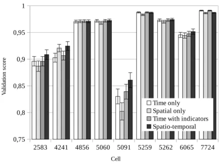
Finally, the third case study looks at predictive approaches from a net-work perspective: using a publicly available dataset, it tries to predict the future traffic load for a given cellular base station in an urban scenario, ex-ploiting spatio-temporal correlations. This could also be used in 5G network optimization in order to allocate resources foresightedly.

3.1

Predicting the wireless channel

In this section, we present two learning methods to predict the wireless channel gain on a long-term scale, without any inputs other than the time-averaged Received Signal Strength Indicator (RSSI). This prediction is per-formed by the Base Station (BS), which is the only fixed element in the network; the BS can indirectly learn the mobility patterns of the mobile users and the fading characteristics of the channel by observing patterns in their RSSI. Most of the efforts in the literature have focused on Multi-Input Multi-Output (MIMO) techniques on short time horizons, but several works [74] [75] have expressed the need for long-term accurate channel gain predictions. The two machine learning techniques we use in this context are GB models and SVR machines . The GB model can be used as a baseline, as it does not try to generalize its experience, but simply considers each class as a separate classification problem. SVRs are able to find and generalize patterns in the data, making better predictions with fewer data.1

3.1.1

State of the art

Wireless links are often modeled as Rayleigh fading channels. Most model-based prediction systems concentrate on short-term predictions of the fading envelope for wideband channels [77], and cannot be directly used for opti-mization at the higher layers.

1_{The work presented in this section was presented at IEEE ICNC 2017 and published}

Shen et al. predict future channel quality from receiver-side Channel State Information (CSI) [78], but the auto-regressive filters they use are only accurate on a timescale of a few milliseconds. The work in [79] proposes a prediction method tailored to Orthogonal Frequency Division Modulation (OFDM) and based on time-domain statistics with a slightly longer range, but the timescales for accurate predictions are still far below 100 ms.

Another auto-regressive model is proposed by Jarinova [80], but its pre-dictions are extremely short-range and the order of the filter is a parameter that needs to be optimized carefully.

Several studies in the literature have attempted to solve the long-term channel prediction problem with machine learning techniques. A typical example is Ramanan and Walsh’s channel prediction algorithm for sensor networks [81]; it is a distributed algorithm that employs message passing techniques to minimize the Kullback-Leibler divergence between the expected prior distribution and the actual posterior.

The problem of channel prediction is central in Cognitive Radio (CR) systems, and Demestichas et al. propose a GB model [82] to solve this issue. Their GB network predicts the future capacity for each possible CR configuration, and adapts to channel conditions online, but it is meant for Modulation and Coding System (MCS) selection rather than for optimization at higher layers.

Flushing et al. take an empirical approach [83], combining a probing mechanism with SVR to predict link quality in dense wireless networks. Thanks to mobility, the probing system can learn about several different topologies and extend this knowledge to larger, denser networks.

Finally, Liaoet al. perform long-term channel prediction [75] using both spatial and temporal information. The authors propose a Gaussian Process (GP) regression, training the system through a series of routes on a city map. Their prediction method is robust against spatial errors, with better perfor-mance than both SVR and auto-regressive filters. Although their method is sound for large-scale scenarios, it does not deal with smaller cells and needs Global Positioning System (GPS) information from clients, which might not be available.

3.1.2

Studied scenario

As we mentioned in Section 3.1, we used a GB model and an SVR to pre-dict the future RSSI of a wireless channel, without external inputs such as GPS data. The two learning methods were trained on the same RSSI data, generated by simulating a realistic urban scenario. The wireless channel we considered used a 945 MHz downlink carrier frequency (one of the commer-cial bands used in Long Term Evolution (LTE)), and the users moved in a Manhattan grid of 100 buildings.

The grid we used is composed of 20 m wide square buildings, with 10 m wide one-way streets at each corner. The evolved Node Base (eNB) is placed at coordinates (140,140), on top of a building close to the center of the simulation area.

Propagation loss and fading The propagation loss was computed with the open-source system-level network simulator ns–3 [84]. In particular, we used the LTE module [85] and a radio propagation model called Hybrid Buildings Propagation Loss Model, which chooses the correct propagation model based on the reciprocal position of transmitter and receiver (both outdoors, both indoors, only one indoors). This model also takes into ac-count the external wall penetration loss (for different types of buildings, i.e., concrete with windows, concrete without windows, stone blocks, wood), and the internal wall penetration loss.

We used the ns–3 simulation to create a square grid of path loss measures in our urban scenario, with a sampling distance of 33 cm. The path loss was then approximated as a linear combination of the 4 closest points in the grid, weighted by the relative distance. The main parameters of the ns–3 simulation are listed in Table 3.1.

The fading and shadowing processes were both simulated from well-known models. We used the log-normal model for shadowing, with a standard devi-ation of 4 dB and a correldevi-ation distance of 8 m. Doppler fading was modeled with a Rayleigh distribution, using the parameters listed in Annex B.2 of [86] and the Welch periodogram method. In the fading calculation, the node

150 200 250 x (m) 120 140 160 180 200 220 240 y (m) (a) Pedestrian 100 150 200 x (m) 60 80 100 120 140 160 180 200 y (m) (b) Vehicular

Fig. 3.1: Examples of trajectories for the two mobility models.

speed was assumed to be constant, simplifying the computation significantly with negligible error.

Mobility model We used two mobility models: pedestrian and vehicular. In both models, the user goes from point A to point B by choosing the direction that takes them closer to point B at each intersection.

In the pedestrian model, a person walks at a constant speed of 1.5 m/s along the side of the nearest building at a distance of 0.5 m. Road crossings are placed at each intersection, and the pedestrian waits for a random time

Parameter Value

Downlink carrier frequency 945 MHz

Uplink carrier frequency 900 MHz

Resource block bandwidth 180 kHz

Available bandwidth 25 RB

eNB beamwidth 360◦ (isotropic)

TX power used by the eNB 43 dBm

eNB noise figure 3 dB

Number of buildings 100

Floors for each building 5

Radio Environment Map resolution 9 samples/m2

2 2.5 3 3.5 4 4.5 5 0.5 1 1.5 2 2.5 3 3.5 4 4.5 5 RMSE (dB) Distance (s) Pedestrian (1 s step) Bayesian (memory: 1) Bayesian (memory: 2) SVR (memory: 1) SVR (memory: 3) SVR (memory: 5)

Fig. 3.2: Prediction error for the pedestrian scenario (1 s window).

between 0 and 5 seconds before crossing to wait for cars.

In the vehicular model, the driver keeps a constant speed of 15 m/s while driving straight, switching between the 3 lanes by moving at a 45 degree angle. Before a turn, the driver switches to the correct lane (e.g., they switch to the right lane before turning right), then slows down to 5 m/s with a constant deceleration in the 5 meters before the curve and makes a circular turn. After reaching the destination, the driver stops and reverses to slowly park on the curb, with a semi-circular trajectory.

The channel data were generated by running the urban scenario 5000 times for the pedestrian model and 10000 for the vehicular model, obtaining 3-4 days of data for the vehicular model and 20 hours for the pedestrian model (the car reaches its destination faster, so the traces are shorter). Two example trajectories for both models are shown in Figure 3.1.

3.1.3

Learning parameters and results

Both prediction methods were trained on the full available dataset, with two different sampling rates: the channel was averaged over a window of 1 s and 0.5 s.

3.5 4 4.5 5 5.5 6 6.5 7 7.5 8 0.5 1 1.5 2 2.5 3 3.5 4 4.5 5 RMSE (dB) Distance (s) vehicular (1 s step) Bayesian (memory: 1) Bayesian (memory: 2) SVR (memory: 1) SVR (memory: 3) SVR (memory: 5)

Fig. 3.3: Prediction error for the vehicular scenario (1 s window).

The Bayesian model used a Gaussian prior, centered on the last known channel sample; the probability vector for all classes was multiplied by a factor k to obtain the Dirichlet parameter vector α. Both the prior weight factor k and the variance σ of the Gaussian distribution were optimized as hyperparameters by cross-validation. The channel quantization step used to divide the data into classes was 2 dB.

As regards the SVR learning algorithm, we found the Radial Basis Func-tion (RBF) kernel: k(zi,zj) = e−γ||zi−zj||

2

to perform best with respect to other possible kernel choices. In this case, the hyperparameters of the model are γ and C in (2.9): a grid search on (γ, C) pairs was thus performed, and the one with the best cross-validation Root Mean Square Error (RMSE) was selected.

After cross-validation, the performance of both prediction methods was measured on a previously unknown test set.

Figure 3.2 shows the prediction RMSE for the pedestrian mobility model; the quality of the prediction is very good even with the simpler model, as pedestrians are slow and generally highly predictable. As expected, SVR clearly outperforms the naive Bayesian model, as it is able to generalize its experience and to better capture the features of the model. The gain

2 2.5 3 3.5 4 4.5 5 0.5 1 1.5 2 2.5 3 3.5 4 4.5 5 RMSE (dB) Distance (s) Pedestrian (0.5 s step) Bayesian (memory: 1) Bayesian (memory: 2) Bayesian (memory: 3)

Fig. 3.4: Prediction error for the pedestrian scenario (0.5 s window).

of the longer memory is less pronounced for the Bayesian model, as it is overshadowed by the small size of the dataset (a longer memory means that a bigger dataset is necessary, and the memory-3 Bayesian model is not plotted, as its performance is not better than that with memory 2).

In the vehicular scenario, the RMSE is higher and the performance gap between the two methods is smaller (see Figure 3.3); the Bayesian model even outperforms the SVR if the prediction is more than 3 seconds ahead, but a prediction error of more than 7 dB is only slightly better than no prediction at all (the prediction RMSE when using a memoryless channel model is about 8 dB). This may be due to the high speed of the vehicles (∼ 10 times the speed of the pedestrians), which makes accurate generalizations about the evolution of the channel hard.

Figures 3.4 and 3.5 show the performance of the Bayesian method with a channel sampling window of 0.5 s; due to the computational cost of the SVR training, its performance in this case has not been evaluated. The figures show that the trend in the performance of the Bayesian method is essentially the same, although the error is higher; the performance of the memory-3 Bayesian model shows that a longer memory is beneficial for the pedestrian model, but loses most of its benefits in the more chaotic vehicular scenario

3.5 4 4.5 5 5.5 6 6.5 7 7.5 8 0.5 1 1.5 2 2.5 3 3.5 4 4.5 5 RMSE (dB) Distance (s) Vehicular (0.5 s step) Bayesian (memory: 1) Bayesian (memory: 2) Bayesian (memory: 3)

Fig. 3.5: Prediction error for the vehicular scenario (0.5 s window).

unless a bigger dataset is used.

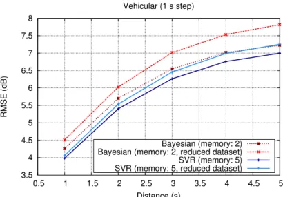
Finally, Figure 3.6 shows the performance of the two predictors when they are trained with a reduced dataset: the two predictors were trained on 20% of the available data in the vehicular scenario with a 1 second step. The plot shows how the performance of the SVR degrades far less than that with the Bayesian model, thanks to the former’s ability to generalize experience. In fact, the reduced-dataset SVR performs better than the full-dataset Bayesian model when the prediction distance is less than 5 seconds.

The training was performed with just a few hours of RSSI data, so a BS with multiple connected users might be able to quickly gather the necessary training data and achieve a high-quality prediction in a very short time. However, the computational cost of the training itself is not negligible; while SVRs show a clear performance gain in both scenarios, the Bayesian model might be enough for applications that need a lower precision. It is worth noting that the SVR can have a satisfactory performance even when trained using a reduced dataset, as shown in Figure 3.6; this makes it ideal if the limiting factor is not computational capability, but the size of the available dataset (e.g., in adaptive systems that are trained online to follow a time-varying scenario). The quality of the predictions is generally high, and the

3.5 4 4.5 5 5.5 6 6.5 7 7.5 8 0.5 1 1.5 2 2.5 3 3.5 4 4.5 5 RMSE (dB) Distance (s) Vehicular (1 s step) Bayesian (memory: 2) Bayesian (memory: 2, reduced dataset) SVR (memory: 5) SVR (memory: 5, reduced dataset)

Fig. 3.6: Prediction error for the vehicular scenario (1 s window) including results using a reduced dataset.

RMSE is almost as low as the results shown in [75], but without the use of GPS data, thereby reducing the energy consumption.

3.2

Predicting battery usage in smartphones

As of today, most devices predict the battery depletion time by taking into account the mean duration of a full battery charge and the most recent battery-draining trend, disregarding time and location information [73]. In this section, we propose a novel method for the prediction of the battery depletion time that makes use of a NN to draw a personalized battery-usage pattern from time and location information provided by the mobile device. We apply our method to a dataset that includes mobility data collected by the LifeMap monitoring system at Yonsei University in Seoul [87]. Results show that our prediction method is by far more accurate than a popular method, currently employed in commercial mobile devices to predict the residual duration of the battery charge, and outperforms other machine-learning methods. We also provide insights on the importance of location information to the accuracy of such a prediction, and on the computational

complexity of the proposed approach.2

3.2.1

State of the art

Several machine learning techniques have been applied to predict the battery charge duration of mobile devices. Most of the proposed solutions based the forecast on the current state of the device together with the battery-discharge history. For example, Zhao et al. [73] use the multiple linear regression prediction method: the discharge rate is calculated by comparing the current device status (e.g., CPU load, LCD brightness and I/O device usage) with the discharge rates that were observed in the past.

In [89], two NNs are trained in order to predict the discharging curve of batteries. Starting from some considerations on the electro-chemical nature of rechargeable batteries, the authors derive a non-linear discharging pattern. In order to model this behavior, they feed the NNs with some key parameters of the battery and device state, such as time, battery level, battery tempera-ture, and resource usage in the past. The obtained predictor can estimate the remaining working time with an accuracy of 3%. However, their model was implemented and evaluated on a digital multimeter under controlled research conditions and no testing was performed on real world data. Wenet al. [90] propose to predict battery lifetime by using an online and offline calculation. First, a reference discharge curve is derived from a one-time, full-cycle, volt-age measurement of a constant load, and is suitably transformed to reduce prediction complexity. Then, the forecasting is performed by mapping the current discharging data on the reference curve, using linear fitting or Least Squares methods.

An empirical approach to battery lifetime prediction is proposed in [91]. After analyzing a large dataset containing the discharging patterns of several users and training a general model, they built a tool to predict smartphone charge levels by classifying smartphone users based on the comparison of their discharging patterns with those in the dataset.

2_{The work presented in this section was presented at IEEE GLOBECOM 2017 and}

In [92], Rakhmatov et al. study the problem of battery discharge time prediction from a theoretical point of view. Starting from the physical work-ing principles of a lithium-ion electrochemical cell, a high-level model of the battery is built. The discharging coefficients of the model are estimated by simulation and statistical fitting of empirical data, and variable and constant loads are taken into account to improve the estimate of the residual operating lifetime of the device.

Most of the techniques mentioned above do not take individual users’ discharging patterns and personal behavior information into account, but instead exploit the depletion discharging curve of a generic smartphone usage or focus on a short-term prediction mainly employing low-level information. Although current battery level and resource usage are fundamental to predict the battery discharge time, we advocate that a much more reliable and long-term estimation of the battery charge can be obtained by considering some space-time features of the device usage patterns. Our model will be able to capture time- and location-dependent user habits which can have a heavy impact on the battery lifetime [73]. Moreover, it is highly scalable to different types of devices and batteries and does not require manual tuning or reference parameters, unlike [90] or [73].

3.2.2

Data analysis

In this section, we discuss the proposed estimation method, the dataset we used and the selection of input and output parameters. Then, we explain the preprocessing operations performed on the data to ease the learning task of the NN.

Dataset and features The dataset from the LifeMap project [87] includes a wide collection of mobility data that was gathered from the smartphones of 6 graduate students from Yonsei University over 6 months. More specif-ically, data about the battery level, position and connectivity level of each smartphone were retrieved from the operating system and stored every 10 minutes. Data clearly span many charge and discharge cycles, but the

bat-tery charge reached a critically low level only on a few such cycles, since in many occasions the smartphones were recharged during the day, before the battery charge dropped below critical levels. Therefore, given this limitation of the dataset, we rely on the expected lifetime of the battery, as we will explain in the following paragraphs.

To design our predictor, we first need to identify the features, or input

parameters, that have to be extracted from the dataset, and the targets, or

output values, of the machine learning model. The choice of these parameters is discussed in the following.

Target parameter Since our purpose is to predict the battery discharge process over time, the output of the estimator should be a projection of the residual lifetime of the device in the future. To build the training set for our machine learning algorithm, hence, we need to find the (expected) residual lifetime of the battery charge in each of the time instants of the discharge phases where data were collected. For the discharge phases that end with a non-negligible residual battery level, the expected depletion time is estimated by linear extrapolation of the charge levels during that cycle. More specifi-cally, let (t0, t1, . . . tn) be the set of sample times in a given discharge period, andb(ti) be the value of the battery level (on a 0-100 scale) measured at time

ti, i = 0,1, . . . , n. If we take the whole discharge cycle into consideration, the expected depletion time is obtained as:

tdep =t0−b(t0)

tn−t0

b(tn)−b(t0)

. (3.1)

Finally, the outputs yi used to train our prediction model are obtained for each discharge cycle as

yi =tdep−ti, 0≤i≤n . (3.2) An example of this analysis is shown in Figure 3.7. We observe that this estimate is more accurate when b(tn) is small, i.e., when the discharge cycle ends with an almost complete discharge of the battery, which is quite

10,000 20,000 30,000 40,000 50,000 60,000 0 20 40 60 80 100 System time [s] Battery lev el [%] Linear fit Discharge cycle

Fig. 3.7: Example of battery discharge rate estimation.

common for modern devices [72]. The linear estimation of the depletion time is a limit to the prediction accuracy, but the limit is inherent in the dataset. Moreover, we observe that the estimate of the residual battery charge duration is more accurate when it becomes more useful, i.e., when the battery level is low.

Input features Our model considers multiple inputs in order to estimate the remaining battery lifetime, namely:

• Battery level: the current status of the battery is clearly essential for a meaningful prediction.

• Time of the day: this parameter is essential to allow the model to learn and recognize specific battery usage patterns during the day. For instance, a user may make a more intensive use of the smartphone while resting in the evening, rather than during the day, or vice versa. To capture these aspects, battery usage data need to be coupled with time information.

• Day of the week: along the same rationale, this feature can make the NN able to recognize patterns of battery usage that depend on the day of the week. For example, sports activities regularly practiced during the week may be associated to a lower usage of the smartphone (e.g., when left in the locker) or to a higher usage (e.g., due to activity-tracker applications), depending on the user’s habits.

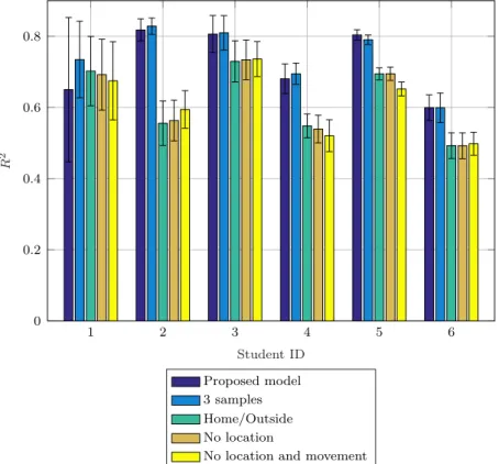
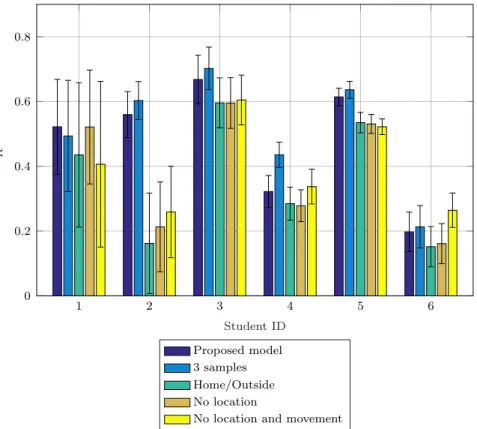
• Location: this feature can also discriminate different battery consump-tion patterns, which are often correlated with the user’s locaconsump-tion. The dataset includes data regarding the user movements and labels for each place that was visited. The locations are classified in 12 categories, such as home, workplace, leisure place, and so on.

• Movement: finally, we consider a boolean feature indicating whether the user is moving from one place to another or is static. This allows us to identify activities typically performed by users while moving on foot or with public transportation, e.g., phone calls or web browsing.

We advocate that such features should be sufficient to discriminate among the specific usage patterns of the different users, thus making it possible to customize the prediction engine.

Preprocessing To efficiently train the machine learning models, we first need to preprocess the input data [93]. In particular, we standardize features and outputs by removing the mean and scaling the amplitudes to get unit variance. By doing so, the distribution of individual features is close to the normal distribution with zero mean and unit variance.

The performance of these methods has been evaluated in terms of the coefficient of determinationR2_{, which is a very popular criterion to measure}

the performance of statistical models [94]. Denoting by yi and ˆyi the actual and predicted values of the ith output, respectively, and by ¯y the mean of the actual values, then the coefficient of determination is defined as

R2 = 1− ∑ i(yi−yˆi) 2 ∑ i(yi−y¯)2 . (3.3)

Note that R2 ≤ 1 and the fraction gives the mean squared estimation error over the variance of the outputs. A perfect predictor will yield R2 _{= 1,}

while a “dummy” prediction that always returns the expected value of the output, disregarding all inputs, would yield R2 _{= 0.}

In our tests, a NN with at least one month’s worth of training data always outperformed all other methods and thus turned out to be the most suitable tool for battery discharge prediction. The parameters of the NN were chosen by performing an exhaustive search in the parameter space; each setting was evaluated by cross validation, and successive rounds refined the search space until convergence. The explored parameters were the size and shape of the hidden layers of the network, the activation function of hidden neurons and the regularization parameter α. We always used the “L-BFGS” [95] solver, an optimizer in the family of quasi-Newton methods, with 200 training iterations. Table 3.2 shows some of the selected configurations; the identity activation function is the simple f(x) = x, the logistic function is given by

f(x) = 1/(1 +e−x), and the Rectified Linear Unit (ReLU) is f(x) = x if

x >0,f(x) = 0 otherwise.

We also report the R2 _{score on the training and validation sets. The}

activation function and network structure strongly impact both the network prediction performance and the time required to train the network. The time

Architecture α Time [s] R2 (val.) R2 (train)

(100, 100, 100, 100 - identity) 0.01 2.479 0.036 0.040 (300 - logistic) 1e-05 2.212 0.036 0.040 (100, 100, 100, 100 - logistic) 0.01 1.064 0.000 0.000 (300 - ReLU) 0.001 40.875 0.580 0.738 (100, 100, 100 - ReLU) 0.01 54.795 0.656 0.842 (100 - tanh) 0.01 17.947 0.568 0.699 (300 - tanh) 0.01 57.476 0.529 0.642 (100, 100, 100 - tanh) 0.01 76.726 0.754 0.853 (200, 150, 100, 50 - tanh) 0.12 111.439 0.806 0.904

Table 3.2: Performance of the NN for different parameter settings. The architecture column contains the number of nodes in the hidden layers of the NN and the activation function.

required to perform the prediction is not listed in the table, since it is always lower than 100 µs.

We found that a distribution of the neurons across several layers allowed the model to detect more complex battery usage patterns, yielding in general better performance, as reporte