Neural networks and support vector machines based bio-activity classification

Neural Networks and Support Vector Machines Based Bio-Activity

Classification

Jehan Zeb Shah∗, Naomie bt Salim

Faculty of Computer Science & Information Systems, Universiti Teknologi Malaysia, 81310 UTM Skudai, Johor, Malaysia.

Abstract

Classification of various compounds into their respective biological activity classes is important in drug discovery applications from an early phase virtual compound filtering and screening point of view. In this work two types of neural networks, multi layer perceptron (MLP) and radial basis functions (RBF), and support vector machines (SVM) were employed for the classification of three types of biologically active enzyme inhibitors. Both of the networks were trained with back propagation learning method with chemical compounds whose active inhibition properties were previously known. A group of topological indices, selected with the help of principle component analysis (PCA) were used as descriptors. The results of all the three classification methods show that the performance of both the neural networks is better than the SVM.

Keywords: radial basis functions, multiple layer perceptron, enzyme inhibitors, classification, chemoinformatics.

1.0 Introduction

Drug discovery is a complex and costly process, with the main bottlenecks being the time and costs of finding, making and testing new chemical entities (NCE). The average cost of creating a NCE in a major pharmaceutical company was estimated at around $7,500/compound [1]. For every 10,000 drug candidate synthesized, probably only one will prove to be a commercial success and there may be 10-12 years after it is first synthesized before it reaches the market [2]. In order to reduce costs, pharmaceutical companies have had to find new technologies to replace the old “hand-crafted” synthesis and testing of NCE approaches.

Currently, many solution- and solid- phase combinatorial chemistry (CC) strategies are well developed[3]. Millions of new compounds can be created by these CC based technologies but these procedures have failed to yield many drug candidates. Enhancing the chemical diversity of compound libraries would enhance the drug discovery. A diverse set of compounds can increase the chances of discovering various drug leads and optimization of these leads can lead to better drugs. In order to obtain a library of great chemical diversity, a number of structural processing technologies such as diversified compound selections, classification and clustering algorithms have been developed.

The classification of drug-like compounds in general into their activity groups using computational methods such as neural networks can make the early filtering and screening

process in drug design faster and less costly[4]. Godden et al [5], have used a median partitioning based method to classify a small number of compounds containing very diverse set of activities like enzyme inhibitor, receptor agonist and antagonist and synthetic and naturally occurring molecules. In [6] support vector machines and a two layer neural network trained with back propagation and some other learning methods were tested for the prediction of drug- non drug compounds from a pool of around 10,000 compounds of which about half were drugs and half non-drugs, collected from various databases. They also analyzed the performance using various types of descriptors. Their study shows that the performance of the SVM is slightly better than neural networks but could not give enough evidence to conclude that SVM outperforms neural networks. In another study, a Kohonen based neural network was used to study the classification of substrate and inhibitors of P-glycoprotein [7]. In this paper we present a study in which neural network methods such as multi layer perceptron (MLP), radial basis functions networks (RBFNs) and support vector machines (SVM) are used for the classification of a number of enzyme inhibitors like angiotensin converting enzyme (ACE) inhibitors, phosphodiesterase enzyme (PDE) and steroid 5α reductase enzyme (SRE) inhibitors. The rest of the paper is organized into four sections. The next section describes the dataset in more detail. Section 3 and 4 deals with the descriptors and methods of classification used in this work respectively. In section 5 the results are presented and the last section concludes the work.

1.1 Datasets And Descriptors

The dataset: The experimental dataset developed for this work composed of three types of

inhibitors, namely ACE, phosphodiesterase enzyme and steroid 5α reductase enzyme inhibitors. The ACE inhibitors are very useful drugs in heart diseases like high blood pressure, heart failure, and also in diabetes for the preservation of the kidney function. ACE enzymes activates a hormone in human bodies called angiotensine which causes blood vessels to constrict and so results in high blood pressure and a strain on the heart[9].The phosphodiesterase inhibitors can be used for blocking one or more of the various subtypes of the enzyme phosphodiesterase. Currently, they are under active research to be used in humans for the treatment of various diseases and some of them have already been tested on human. A current study show that the use of phosphodiesterase III inhibitors in heart failure patients resulted in increased mortality rates[10]. Defects in the steroid 5 -reductase type 2 enzyme activity cause decreased formation of dihydrotestosterone (DHT) from testosterone (T) which increases the T/DHT ratio, resulting in defective masculinization of external genitalia [11]. A number of inhibitors are available to stop this effect.

The compounds used in this work, were obtained from the MDL’s MDDR database. A number of filters were applied to remove the compounds which are redundant due to their exhibition of multiple activities. The compounds for which the descriptors could not been generated due to some error in their structural data were also eliminated. After filtering, the dataset contained 314 ACE inhibitors, 792 phosphosdiesterase (including subtypes I and III) inhibitors, and 244 steroid 5 -reductase (subtype I and II) inhibitors.

Generation of Descriptors: The descriptors generation or features extraction is an important

step in computational classification of molecular structures and other problems such as clustering and quantitative property/activity relationship modeling. A number of modeling tools are available that can be used to generate structural descriptors. In this work, we use the

Dragon software to generate around topological indices for the molecules. Topological indices are a set of features that characterize the arrangement and composition of the vertices, edges and their interconnections in a molecular bonding topology. These indices are calculated from the matrix information of the molecular structure using some mathematical formula. These are real numbers and possess high discriminative power and so are able to distinguish slight variations in molecular structure. This software can generate 99 topological indices which includes Zagreb index, quadratic index, Narumi simple topological index, total structure connectivity index, Wiener index, balaban index and etc.

Scaling of the variables generated is very important in almost all computational analysis problems. If magnitude of one variable is of larger scale and the other one is of smaller scale then the larger scale variable will dominate all the calculations and effect of the smaller magnitude variables will be marginalized. In this work all the variables used were normalized such that the maximum value for any variable is 1 and the minimum is 0.

In order to reduce the descriptor space and to find the more informative and mutually exclusive descriptors a feature selection method principal component analysis (PCA) [12] was used. PCA was carried out using the MVSP 3.13 [13]. It has been found that 10 components can represent more than 98% of the variance in the dataset. The input to the neural networks and SVM is thus a 10 X 1350 data matrix.

2.0 Materials and Methods

2.1 Neural Networks

In this study, two important supervised neural networks, the feed forward multilayer perceptron and the radial basis function network methods are used for the classification of chemical inhibitors.

2.2 Multi Layer Perceptron(MLP)

The multilayer perceptron is a static feed forward neural network that can have virtually any number of hidden layers besides the essential input and output layers of neurons. Practically one or two hidden layers are enough to model complex systems [14, 15]. Usually the error backpropagation [16] method is the preferred learning method to train the network. In such learning the error yielded at the output neuron is propagated back along the layers of the network and the weights are corrected. The output is compared with the desired output of the sample presented at the input. The error Ei(t) for the output neuron i and a given input sample is given as: (1) ) ( ) ( ) , (w t d t y t E_i = _i − _i

where di is the desired output and yi is the observed outputof neuron i at time instant t of the training process. The observed output yi of a simple three layer network with one output neuron can be given as:

(2) ) ) ( . ( 1 1 0 0

∑

∑

where g and h are the activation functions of the output and hidden layer neurons respectively. The exponent n and m represents the total number of neurons in the hidden and input layers respectively, and w’s are the weights and zk is the input example.

Using the theory of gradient descent learning, each weight in the network is updated by correcting the present value of the weight with a term proportional to the error at the weight, given as (3) ) ( ) ( ) ( ) 1 (t w t t z t wkj + = kj +ηδj k

where η is the learning rate parameter whose value is between 0 and 1. δ is the value of local error propagated from the output error Ei(t).

The back propagation is a gradient descent minimization procedure used to minimize the cost functional of the feed forward neural network which is a function of the weights of the network and these weights are changing with time. So, the backpropagation learning algorithm tries to find minimum point on the surface formed by the weights of the network. Since all the error computations are based on the local information of the dataset and network, it is always likely that the learning process may trap in local minima. In order to avoid local minima, a momentum term can be used

(4) ) ( ) ( ) ( ) ( ) 1 (t w t t z t w t w_kj + = _kj +ηδ_{j k} +μΔ _kj

where μ is the momentum constant which can have values between 0 and 1, Δw is the change in weight in iteration t and t-1.

The search for the parameters η and μ is a trial and error problem. In [17, 18] a method based on the fuzzy inference system is used to change these parameters adaptively as the learning process progress. This method enables the learning process to avoid the local minima as well as results in faster convergence.

2.3 Radial Basis Function (RBF)

The radial basis function network is a three layer feed forward fully connected network, which uses radial basis functions as the only nonlinearity in the hidden layer neurons. The output layer has no nonlinearity. Only the connections of the output layer are weighted whilst the connections from the input to the hidden layer are not weighted [14, 19]. The activation function of the hidden layer can be expressed as:

[

]

Where zk , mi, and σi are the input training sample, centre of the ith Gaussian, and width of the

ith Gaussian respectively. These functions are called the radial basis functions and the final output is the sum of the connection’s weight times these functions.

(6)

∑

The training process is similar to the one for back propagation network, where a cost function like (1) is iteratively minimized. The cost function is a function of the weights in the output layer, the centroids and widths of the radial basis functions. The learning process is not implemented as single procedure, but rather three step procedures are adapted. First the centroids of the radial basis functions are determined using a clustering method like K-means, second the receptive width σi are determined using heuristic p-nearest neighbors method and last the weights of the final layer are determined simply by a linear least square regression [19].

2.4 Support Vector Machines

Support vector machines have recently found considerable attention in classification problems due to its generalization capabilities. These classifiers maximize the distance (margin) between the training examples and the decision boundaries by mapping the training examples to higher dimensional space [20, 21]. The dimension of the new space is considerably larger than that of the original data space. Then the algorithm finds the hyperplane in the new space having the largest margin of separation between the classes of the training data using an optimization technique known as the risk minimization. For a binary classification problem where there are only two classes in the training datay_i ={−1,1}, a hyperplane can be defined as:

(7) 0 .x+b= W

where W is the normal to the hyperplane and b/W is the shortest distance of the plane from the origin.

For a good classification model the positive and negative examples of the training data should fulfill the following two conditions:

(8) , 1 . , 1 . -1 i y for 1 i y for = + = − ≤ + + ≥ + b x W b x W i i

These inequalities can be combined into one set of inequalities

(9)

i

for

∀

The SVM finds an optimal hyperplane responsible for the largest separation of the two classes by solving the following optimization problem subject to the condition in (9)

(10) 21 , W W Min T b w

The quadratic optimization problem of (9) and (10) can be solved using a langrangian function (11) ) 1 ) . ( ( . ) , , ( 1 2 1

∑

where αi are the constants known as langrange multipliers. The solution of (11) for αi determines the parameters w and b of the optimal hyperplane. We thus obtain a decision function for the binary classification as:

(12) ) , sgn( ) ( 1

∑

In any classification task only a few langrangian multipliers αi tend to be greater than zero and the corresponding training vectors are the closest to the optimal hyperplane and are called the support vectors. In nonlinear SVM, the training samples are mapped to a higher dimensional space with the help of a kernel function K(xi ,xj ) instead of the inner product <xi

, xj > . Some of the famous kernel functions are the polynomial kernels, radial basis function kernels, and sigmoid kernels[21].

3.0 Results and Discussion

and the enzyme inhibitors in particular. A number of neural networks strategies have been applied to find the best networks for the feed forward MLP and RBF neural networks which are then compared with best SVM model obtained.

All the classifiers were used in this work for multiple target classifications and the number of targets was the three classes, i.e. various types of inhibitors used in this work.

The dataset have been partitioned into two parts: a training part which is used for training of the algorithm and a test part which is used for testing. The percentage of training and testing portions of the dataset was varied in order to study the variation of performance caused by change in the ratio of training to testing partitions of dataset. The training/testing partitions used contain (10%, 90%), (30%, 70%), (50%, 50%), (70%, 30%) and (90%, 10%) of the dataset. For the selection of samples in training and testing portions, interleaved method was used to make it sure that percentage of each class in each portion is preserved.

In this work two types of neural networks, feed forward neural network and a radial basis function neural networks with one hidden layer were considered. The networks were tested for a variable number of hidden layer neurons. The number of input layer neurons was the same as the number of inputs which correspond to the number of variables in the dataset and in the output layer there were three neurons corresponding to the three target outputs. The output can range between (0, 1). The training samples were presented to the neural networks, the output was compared with the desired output for a given input sample and the errors were back propagated for the update of weight vectors.

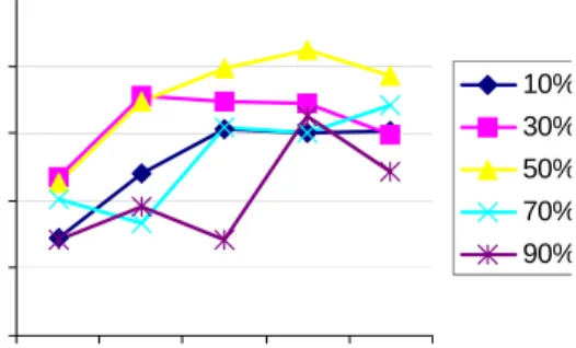
First the experiments were carried out for various numbers of neurons in the hidden layer. In both types of neural networks, it has been observed that the performance increases with the increase in number of neuronal nodes. It has been found that performance starts degrading after reaching a steady state point. Figure 1 and Figure 2 shows the behavior of MLP and RBF networks for various values of neurons in the hidden layer. In both the cases the best results were obtained when the number of hidden layer nodes was 20.

72 75 78 81 84 87 5 10 15 20 25

No. Hidden Layer's Neurons

%A c c u rac y 10% 30% 50% 70% 90%

Figure 1 Prediction accuracy of MLP neural network. The predictions are shown for variable number of hidden nodes for various training data percentage.

62 67 72 77 82 5 10 15 20 25

No. Hidden Layer's Neurons

% A ccu ra c y 10% 30% 50% 70% 90%

Figure 2 Prediction accuracy of RBF neural network. The predictions are shown for variable number of hidden nodes for various training data percentage.

The networks have been trained and tested with variable ratio of samples from the dataset. The behavior of both the network is almost similar. As the training data is increased the accuracy of prediction increases, but it is not good when the number of training examples is very large than the testing examples. The MLP network gives the best prediction accuracy when the training/ testing ratio is 50%, whereas the RBF network prediction is best when it is trained with 10% and tested with 90% of examples in the dataset.

For SVM, the polynomial Kernel was used with various degrees, but the best results were obtained for degree 3 and degree 4 as is shown in Figure 3. As we increase the percentage of the training dataset, the prediction accuracy increases and reaches its highest point at 50% and then decreases. The best average prediction obtained for SVM was 72.83%.

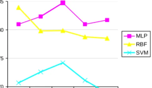
The results for all the three methods are compared as in Figure 4, where the prediction accuracy of neural methods is found to be superior over SVM. The MLP gives the highest correct prediction when trained with 50% of the training data and RBF gives its best result for only 10% of the training data and at this point its prediction accuracy is comparable with that of MLP.

4.0 Conclusion

In this work a number of machine learning methods have been evaluated for the classification of a number of important enzyme inhibitors based on topological descriptors. It has been observed that the generalization abilities of the RBF neural network is superior to MLP as well ,as to SVM where it can give us good performance even for training with only 10% of the dataset. However, it should be noted that polynomial kernel was used for SVM, and its performance may become better with the use of RBF or some other kernel. Overall, the performance of SVM can not be said at par that of neural methods in general as the best performance can not reach to that of neural networks.

65 70 75 10 30 50 70 90 % Training Data % A c c u ra c y

Figure 3 Prediction accuracy of SVM results are shown for various degrees of the polynomial kernel. 70 75 80 85 10 30 50 70 90 % Training Data % A ccu ra c y MLP RBF SVM

Figure 4 Overall Prediction Results for MLP, RBF and SVM. The results shown for MLP and RBF are when the number of neurons in the hidden layer is 20. For SVM, degree for the polynomial kernel is 4.

References

[1] Hecht, P. (2002): High-throughput screening: beating the odds with informatics-driven chemistry. In

Current Drug Discovery, pp. 21-24.

[2] Warr, W.A.: High-Throughput Chemistry: Handbook of Chemoinformatics. Wiley-VCH, Germany 2003. [3] Hall, D.G., Manku, S., Wang, F. (2001) Solution- and Solid-Phase Strategies for the Design, Synthesis, and

Screening of Libraries Based on Natural Product Templates: A Comprehensive Survey. Journal of combinatorial Chemistry 3: 125-150.

[4] Schnecke, V., Bostrom, J. (2006) computational chemistry driven decision making in lead generation. Drug Discovery Today 11.

[5] Godden, J.W., Xue, L., Bajorath, J. (2002) classification of biologically active compounds by median partitioning. Journal of chemical Information and computer science 42: 1263-1269.

[6] Byvatove, E., Fechner, U., Sadowski, J., Schneider, G. (2003) comparison of support vector machines and artificial neural network systems for the drug/nondrug classification. Journal of chemical Information and computer science 43: 1882-1889.

[7] Wang, Y.H., Li, Y., Yang, S.L., Yang, L. (2005) classification of Substrates and Inhibitors of P-Glycoprotein Using Unsupervised Machine Learning Approach. Journal of chemical Information and computer science 45: 750-757.

[8] MDL’s Drug Data Report. Elsevier MDL,

http://www.mdli.com/products/knowledge/drug_data_report/index.jsp [9] ACE Inhibitors: http://www.healthyhearts.com/medications.htm

[10] Amsallem, E., Kasparian, C., Haddour, G., Boissel, J., Nony, P. (2006) Phosphodiesterase III inhibitors for heart failure. The Cochrane Database of Systematic Reviews.

[11] Triaa, A., Hiortb, O., Sinneckera, G.H.G. (2004) Steroid 5-Reductase 1 Polymorphisms and Testosterone/Dihydrotestosterone Ratio in Male Patients with Hypospadias. Hormone Research 61:

180-183.

[12] Jolife, I.: Principal component analysis. Springer-Verlag, New York 1986. [13] MVSP 3.13, Kovach computing services: http://www.kovcomp.com/

[14] Tsoukalas, L.H., Uhrig, R.E.: Fuzzy and Neural Approaches in Engineering. John Wiley and Sons, New York 1997.

[15] Ruck, D.W., Rogers, S.K., Kabrisky, K., Oxley, M.E., Suter, B.W. (1990) The multilayer perceptron as an approximation to an optimal Bayes estimator. IEEE Transactions on Neural Networks 1: 296--298.

[16] Rumelhart, D.E., Hinton, G.E., Williams, R.J. (1986): Learning internal representations by error propagation. In Parallel Data Processing. Eds. Rumelhart, D., McClelland, J., The M.I.T. Press, Cambridge, pp. 318--362.

[17] Shah, J.Z., Husain, S.A. (2004): A fuzzy based adaptive BPNN learning algorithm for segmentation of the brain MR images. In 8th IEEE International Multitopic Conference Lahore, pp. 85 - 90.

[18] Arabshahi, P., Choi, J.J., Marks, R.J., Caudell, T.P. (1996) Fuzzy parameter adaptation in optimization: some neural net training examples. IEEE Computational Science and Engineering 3: 57 - 65.

[19] Leonard, J.A., Kramer, M.A. (1991) Radial basis function networks for classifying process faults. IEEE Control Systems Magazine 11: 31 - 38.

[20] Vapnik, V., Golowich, S., Smola, A. (1996) Support vector method for function approximation, regression estimation, and signal processing. Advances in Neural Information Processing Systems 9: 281–287.

[21] Burges, C.J.C. (1998) A Tutorial on Support Vector Machines for Pattern Recognition. Data Mining and Knowledge Discovery 2: 121–167.