DIPLOMARBEIT
Titel der Diplomarbeit„Statistical Credit Risk Models“
Verfasser
Racko Peter
angestrebter akademischer Grad
Magister der Sozial- und Wirtschaftswissenschaften
(Mag. rer. soc. oec.)
Wien, im November 2007
Studienkennzahl lt. Studienblatt A157
Studienrichtung lt. Studienblatt Internationale Betriebswirtschaftslehre
Table of Contents
List of tables and figures... 2
1. Introduction ... 3
2. Implications of the Basel Accords ... 7
3.1 Discriminant analysis... 11
3.2 Logit and Probit Models... 15
3.3 Hazard models as an extension of traditional logit/probit models... 18
4. Input variables... 21
4.1 Quantitative inputs... 21
4.1.1 Identifying the relevant variables... 23
4.1.2 Dealing with the non-linearity assumption in logit/probit models27 4.1.3. Final variable selection... 31
4.1.4 Variables selected into models... 33
4.2 Inclusion of Qualitative Inputs in Default Prediction... 42
4.3 Combining quantitative and qualitative scores – an illustrative example ... 46
5. Calibration ... 47
6. Model validation... 53
6.1 Validation of the fundamental statistical soundness... 54
6.2 Validation of the discriminatory power... 56
6.3 Validation of the calibration of default prediction models... 62
6.3.1 Calibration validation without default correlation assumption... 63
6.3.2 Calibration validation under the assumption of correlated defaults ... 65
7. Alternative approaches to default prediction ... 66
7.1 Artificial Neural Networks... 66
7.2 Structural Models... 68
7.3 Reduced Form Models... 70
9. Conclusions ... 71
Appendix A – German Abstract ... 73
Appendix B – Curriculum Vitae ... 75
List of tables and figures
Table 1.1: Size structure of firms in the EU and USA
Figure 2.1: Capital requirements for a corporate exposure as a function of the PD Figure 3.1: The process of the linear discriminant analysis
Figure 3.2: Relationship between independent variables (Z) and the eventual score (p) in a logistic regression Figure 4.1: A sample default frequency graph
Figure 4.2: Three sample power curves
Table 4.1: input variables in Altman and Sabato’s SME model for the US Table 4.2: input variables in Fernandes’ Model for Portuguese Companies
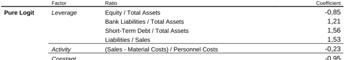
Table 4.3: Input variables for different versions of Moody’s KMV RiskCalc suite for private companies Table 4.4: Variables selected into the pure logit model by Halling and Hayden (2004)
Table 4.5: Variables selected into the hazard logit model by Halling and Hayden (2004) Table 4.6: Altman’s Z-Score model input variables
Table 4.7: Input variables for the quantitative evaluation of a firm in the BA-CA internal rating system Table 4.8: Relative contributions of profitability, leverage and debt coverage factors combined compared to the other factors, sorted by two distinct regions
Figure 4.3: The rating process at Bank Austria Creditanstalt
Table 5.1: One-year aggregate default probabilities for private companies Table 5.1: Master Rating Scales used at Bank Austria Creditanstalt and Erste Bank Figure 6.1: Power curves for various models, as tested by Moody’s KMV Figure 6.2: Three sample ROC Curves
Table 6.1: Available Accuracy Ratios for models discussed throughout the thesis Figure 7.1: The structure of an artificial neural network
4 10 13 17 24 25 33 34 36 39 39 40 40 42 47 48 52 57 58 61 67
1. Introduction
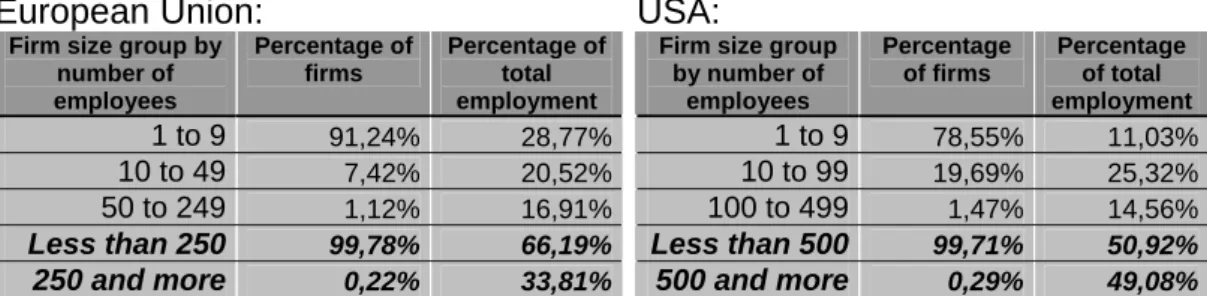
With the implementation of Basel II, banks are faced with more demands on quantifying market, credit and operational risks in their portfolios. Especially the new rules for credit risk quantification, known as Internal Ratings Based Approach, constitute a large part of the entire Basel II Accord. In order to take full advantage of these new rules, banks can, unlike under the old 1988 Basel Accord, implement sophisticated models that capture the individual elements of credit risk in more detail. There are major challenges in the implementation of the IRB Approach, one of them being the internal assessment of the credit risk profile of a bank’s counterparty – a task which has to be accomplished by assigning a default probability to the particular client1. If the counterparty has an assigned rating by an external rating agency, such as Standard & Poor’s or Moody’s, the default probability can be directly obtained from the respective rating as ratings are provided with a default probability percentage for each rating class. However, the majority of companies do not have a rating. For example, on its homepage, Moody’s indicates to have ratings that cover over 11.000 company issuers which is a fairly small figure when compared to the number of companies in the US economy alone – nearly six million. As a result, for those counterparties that do not have a rating, a bank will have to be able to calculate the PD on its own. The vast majority of these firms will be small and middle sized enterprises (SMEs)2. While the exposures of SMEs may not be very large, their importance for every economy is undisputed. There are many arguments that underscore this fact: many new, innovative companies start as small start-ups, SMEs employ a large part of the population and, for example, between 2001 and 2003 in the EU they were a more significant force in driving job growth than their large counterparts3. Therefore, considering how vital these are for any economy it will not only be in the best interest of the bank, as the PD is a major component in the calculation of capital requirements. It will also be in the best interest of each country to have models in place that quantify the default probability as accurately as possible in order to make sure that loans are correctly priced. The following table gives an overview of the size structure of companies in the EU and US as of 2003:
1 Please see Chapter 2 for a more detailed look into the Basel II Accord.
2 In the EU, SMEs are defined as having less than 250 employees and a turnover of less than €50
Million or a balance sheet total of less than €43 Million.
European Union: USA:
Firm size group by number of employees Percentage of firms Percentage of total employment 1 to 9 91,24% 28,77% 10 to 49 7,42% 20,52% 50 to 249 1,12% 16,91% Less than 250 99,78% 66,19% 250 and more 0,22% 33,81%
Firm size group by number of employees Percentage of firms Percentage of total employment 1 to 9 78,55% 11,03% 10 to 99 19,69% 25,32% 100 to 499 1,47% 14,56% Less than 500 99,71% 50,92% 500 and more 0,29% 49,08%
Table 1.1: Size structure of firms in the EU and USA. Sources: Eurostat, United States Small Business Association.
In both the EU and US, SMEs account for well over 90 percent of all companies and employ at least 50 percent of the workforce and thus it is very likely that the credit portfolio composition of most commercial banks will be dominated by SME exposures.
The problem with these firms is that in addition to the fact that they do not possess a credit rating, they also cannot supply any market data that would aid the assessment of their creditworthiness expressed in terms of PD. Instead, they will only be able to provide accounting data. It is an acknowledged fact that market data on firms is much more accurate and reliable than accounting data and in recent years a number of market data based models for credit risk appeared4. The challenge for banks is to be able to quantify credit risk without the knowledge of market data. As a result, the aim of this thesis will be to show the currently prevalent practice of quantifying credit risk in the absence of market data and external ratings where only accounting data can be utilized in the context of Basel II.
Throughout the credit risk literature, William H. Beaver and Edward I. Altman are considered to be the pioneers in the analysis of accounting data with respect to company defaults. Beaver (1966) looked at the effect of individual financial ratios on default and concluded that ratio analysis is useful in bankruptcy prediction. In 1968 E. Altman published his seminal work Financial Ratios, Discriminant Analysis and the Prediction of Corporate Bankruptcy and it is widely considered to be the birth of the so-called statistical credit risk models. It was the first time that multiple ratios were analyzed at the same time in a bankruptcy prediction context as part of the classic Z-Score model. And even though the modelling
technique applied by Altman (1968) has since become outdated, as will be shown in Chapter 3, the framework of current statistical models shares the same idea as the original Z-Score model: a large amount of balance sheet data for many firms that both defaulted and survived over a given period of time is needed to analyze the influence of various factors, mainly financial ratios, on the creditworthiness of borrowers. Afterwards, a selected set of factors that are assumed to have the greatest influence on whether or not a firm defaults, when combined and weighted, will produce a score that will be used to assess the creditworthiness of a particular borrower.
Throughout this thesis, the major aspects and issues of currently used statistical models, most notably logistic models, as a means of quantifying the default probability of exposures will be discussed. These will also be complemented by discussions of already created credit risk models, namely the Z-Score model by Altman (1968), the model for US SMEs by Altman and Sabato (2006), the model proposed by Fernandes (2005), the proprietary RiskCalc model by Moody’s KMV (2000), the model by Bank Austria Creditanstalt AG (2005), Austria’s largest bank, and also a model by Halling and Hayden (2005) which includes a time component in addition to accounting data.
The aforementioned Z-Score by Altman (1968) was the first model to analyze multiple financial ratios in order to assess the creditworthiness of a firm. This model was based on observations of 33 defaulted and 33 non-defaulted manufacturing firms during the period between 1946 and 1965. The asset sizes of these firms range from $0.7 million to $25.9 million, thus omitting large and very small companies. Despite its age and the rather unsuitable functional form in terms of Basel II requirements, this model continues to be somewhat of a benchmark, with authors of other models using it to demonstrate their model’s performance in terms of discriminative ability.
E. Altman and G. Sabato (2006) published a logistic model specifically designed for US SMEs. Using a sample that includes 2010 firms, of which 120 were defaulted, and that spans the time from 1994 until 2002, they mainly attempt to show the importance of having a separate model for assessing the rating of an
SME instead of using a generic model that is also used for large corporations. According to Atlman & Sabato (2006), by taking into account the differences between SMEs and large firms via separate models, banks can lower the required capital according to Basel II.
Fernandes (2005) uses a dataset of 11000 financial statements from Portuguese firms to firstly create two statistical, logistic models, one that takes different industries into account and one without regard for industries. He then uses these models to demonstrate how rating classes can be created from the output of the models.
Moody’s KMV (2000), a provider of credit risk management solutions, also developed a model for PD estimation of unrated private companies, RiskCalc. While some of the details of the model are not disclosed as it is proprietary, Moody’s KMV does provide extensive documentation for RiskCalc. It is not only a good example of a commercially available credit risk model but with its many regional adaptations (there is a RiskCalc version for Australian, Austrian, Belgian, Dutch, French, German, Italian, Japanese, Mexican, Scandinavian, Spanish, UK, and US firms) it also serves the purpose of showing differences in credit risk relevant attributes between countries.
The model by Bank Austria Creditanstalt AG (2005) is a demonstration of an Austrian commercial bank’s internal rating model. While the exact design details are confidential and only available to the bank and its supervisor, it is a good example of how to include qualitative data into a rating model.
Finally, Halling and Hayden (2004) create a model, based on a sample spanning the years between 1994 and 1999 with 2283 firms of which 171 defaulted. This model is unique in that it represents a rare case in which the time component is explicitly taken into account in corporate default prediction. This so-called hazard model is perhaps a glimpse of the future in terms of statistical credit risk models and as such deserves to be mentioned.
The thesis is structured as follows: In Chapter 2, the Basel Accords and their implications on the credit risk assessment of banks’ counterparties are outlined. Chapter 3 deals with the statistical framework that is the basis for models of credit risk and shows which functional form dominates the present landscape, Chapter 4 looks into the issue of identifying the most useful variables for a model, Chapter 5 will outline the process of calibration of models, an area of extreme importance in terms of Basel II compliance, Chapter 6 will detail the validation issues for statistical default prediction models and Chapter 7 will briefly outline alternatives to statistical default prediction. Chapter 8 will conclude.
2. Implications of the Basel Accords
This chapter will outline the main objectives of the Basel Accords, give an overview of the Basel II framework and focus on the implications on the assessment of counterparty credit risk.
The first Basel Accord, drafted in 1988, represented a huge step in banking regulation in that it required banks to hold specified amounts of equity capital. This capital is called regulatory capital and serves the purpose of helping banks absorb losses stemming various risks, credit risk included. For credit risk, the requirement was for a bank to hold 8 percent of risk weighted assets. More precisely, the regulatory capital to be set aside for an exposure would be given by multiplying the exposure amount with a risk weight and then with the 8 percent. The risk weights were set by the Basel Committee and were supposed to reflect the riskiness of certain customer types. For example, the risk weight for an exposure to an OECD country was set to zero percent while an exposure to a corporate received 100 percent. While this regulation certainly helped increase the capital held at banks, weaknesses were soon discovered, most notably the lacking risk sensitivity. This was especially true in the corporate segment: irrespective of whether a borrower was a rated AAA firm or a barely surviving SME, the risk weight remained the same for both borrowers. As a result, in 1999 the Committee began working on the Basel II Accord.
The new Accord indeed incorporates risk sensitivity in both of its main broad methodologies for the calculation of capital requirements for credit risk. The simpler Standardized Approach extends the old Basel I methodology by enabling a differentiation of borrowers according to their external credit rating assessment. As a result, an exposure to a AAA rated customer will result in a 1,6 percent capital requirement, much lower than the 8 percent under the old Accord. However, herein also lays the problem: in order to incorporate this risk sensitivity, external ratings have to be available for a particular borrower. However, as Chapter 1 demonstrated, this will rarely be the case. As a result, the true innovation in terms of adding risk sensitivity into the calculation of capital requirements and achieving a lower capital charge is the Internal Ratings Based (IRB) approach.
The innovation lies in the concept of the bank providing their own estimates of key parameters which are supposed to give a good indication about the overall credit situation of a borrower and his/her exposure:
Probability of default (PD): the quantification of the borrower’s creditworthiness, these estimates have to be provided for a one year horizon. As opposed to the other parameters, the PD is not facility-specific and has to be assigned to every borrower.
Loss given default (LGD): the facility-specific quantification of the amount that a bank will lose once the borrower defaults on a particular exposure.
Exposure at default (EAD): the amount of the exposure at the moment of default of the borrower.
Maturity (M) of an exposure
These key parameters are then used to calculate the capital requirement for each exposure. This is accomplished via the so-called risk weight functions, for which the risk parameters serve as inputs. There are different risk weight functions for different asset classes5, however, since the focus lies on corporate borrowers, only the corporate risk weight functions are presented:
5 Basel II differentiates between the Sovereign, Institutions, Corporate, Retail, Equity,
Correlation (R): ⎟⎟ ⎠ ⎞ ⎜⎜ ⎝ ⎛ − − − × + ⎟⎟ ⎠ ⎞ ⎜⎜ ⎝ ⎛ − − × = −50−×50 −50−×50 1 1 1 24 , 0 1 1 12 , 0 e e e e R PD PD Maturity Adjustment (b):
( )
(
)
2 ln 05478 , 0 11852 , 0 PD b= − × Capital requirement (K):( )
(
)
(
)
⎟ ⎠ ⎞ ⎜ ⎝ ⎛ × − × − + × ⎟ ⎟ ⎠ ⎞ ⎜ ⎜ ⎝ ⎛ − ⎟⎟ ⎠ ⎞ ⎜⎜ ⎝ ⎛ − Φ × + Φ Φ × = − − b b M PD R R PD LGD K 5 , 1 1 5 , 2 1 1 999 , 0 1 1Risk-weighted assets (RWA):
EAD K
RWA= ×12,5×
The main equation is the capital requirement equation (K): its output is the percentage of the exposure at default that has to be set aside for each facility. Besides considering the PD, LGD and M, it also incorporates the effects of asset correlation6 and maturity sensitivity7, through the equations R and b respectively. In addition, the risk-weighted assets (RWA) of an exposure can be calculated by multiplying the capital requirement (K) with the EAD and the inverse of 8 percent, 12,5.
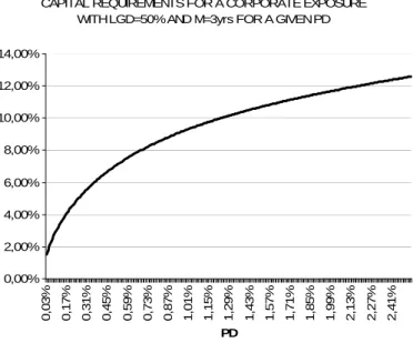
The risk weight functions use the Value at Risk8 concept and were calibrated in
order to obtain a reasonable capital requirement given the estimated input parameters. Figure 2.1 shows the capital requirements, expressed in percentage points, as a function of the default probability for an LGD of 50 percent and a maturity of three years:
6 The main goal is to capture the effect of the overall economic environment on a borrower. 7 The aim is to capture maturity effects. First of all, higher maturities imply higher risk and
secondly, low-PD borrowers have a higher downside potential for downgrades than high-PD borrowers. As a result, an increase in the maturity will have a bigger impact on capital requirements for better rated firms than for worse rated ones.
8 Value at Risk (VaR) is a measure of loss: VaR provides the maximum loss for a given
probability for a given holding period. For example, if the 99 percent, 1 day VaR is € 1.000, it means that with a probability of 99 percent the loss on one day will not exceed € 1.000. The risk weight functions operate with a 99,9 percent confidence interval, i.e. the intention is for regulatory capital to be sufficient in 99,9 percent of all loss occurrences.
CAPITAL REQUIREMENTS FOR A CORPORATE EXPOSURE WITH LGD=50% AND M=3yrs FOR A GIVEN PD
0,00% 2,00% 4,00% 6,00% 8,00% 10,00% 12,00% 14,00% 0 ,03% 0 ,17% 0 ,31% 0 ,45% 0 ,59% 0 ,73% 0 ,87% 1 ,01% 1 ,15% 1 ,29% 1 ,43% 1 ,57% 1 ,71% 1 ,85% 1 ,99% 2 ,13% 2 ,27% 2 ,41% PD
Figure 2.1: Capital requirements for a corporate exposure as a function of the PD
It becomes clear that the estimation of these risk parameters will pose serious challenges to banks applying for the IRB Approach. The Basel Committee acknowledges this fact by enabling the implementation of two variants of the IRB Approach. Under the Foundation IRB, the bank will only have to provide estimates for the PD while under the Advanced IRB, all inputs will have to be estimated by the bank itself. Nonetheless, irrespective of which IRB Approach a bank chooses, the quantification of counterparty credit risk, expressed as the borrower’s PD, will be the bank’s task. This fact also underscores the central importance of borrower PD estimation.
There are several implications for the evaluation of credit risk associated with borrowers using default prediction models arising from Basel II. First of all, the required final output of the credit risk assessment process was clearly specified – the final results obtained from default prediction models will have to be default probabilities. Secondly, the PD will have to be estimated for every corporate borrower in the portfolio and as a result, banks will have to develop models that accomplish this task with the available information at hand. As a result, when no market data is available, models that can work with accounting data as input will have to be implemented. Third, besides providing the risk weight functions, Basel II also specifies an extensive framework under which such models have to be operated and requirements that they have to meet. For example, the models have
to be able to classify borrowers into seven rating classes consistently9, the PDs that are estimated are subject to various rules, the PDs can only reflect borrower characteristics and models have to be validated in regular intervals. Finally, Basel II provided a huge boost for research in the area of credit risk measurement, which at the time was not yet well established and definitely lagging behind that of market risk. This research is mainly the result of the fact that while Basel II clearly defines the parameters and the framework of their use, it does not define how these parameters are to be estimated and which methodologies are to be applied. The subsequent research was aimed at closing this gap.
As a consequence of the entire Basel II regulation, which has had a substantial effect on the way borrower default risk is estimated, the focus throughout this thesis will not only lie in the design and statistical background of the models but also on areas which the Basel Committee emphasizes, such as the calibration of model outputs to PDs, the validation methods which should ensure a correct evaluation of borrower credit risk profiles over longer periods of time as well as the inclusion of qualitative data into models.
3. Modelling framework
This chapter will highlight the methods that can be used in construction of a default prediction model. It will show why in today’s modelling practice logit/probit models are the clear favourites and linear discriminant analysis, as introduced by Altman (1968), is more or less only regarded as an important evolutionary step that nowadays does not find application in banking practice. Moreover, it will be shown why more advanced applications of logit/probit models are not being considered.
3.1 Discriminant analysis
Linear discriminant analysis is used to find a linear combination of various features and characteristics of a dataset that differentiates best between two or more classes within this dataset. In the context of credit risk, this means that in
order to perform a discriminant analysis, one first needs data from both non-defaulted and non-defaulted firms as these will be the two groups to be differentiated. This data should contain financial/accounting variables. They are the independent variables and discriminant analysis attempts to find a linear equation that includes these variables such that, based on the outcome/score of the equation, the clearest and best differentiation between the two groups can be made. More formally, the equation will have the following form:
e X b X b X b a Z = + 1 1+ 2 2 +K+ n n +
Here, Xn is the value of the independent variable n, bn is the coefficient for the
independent variable n (i.e. the main result of the analysis), a is the constant, e is the error term and Z is the dependent variable based on which the classification into the two groups is done. As can be seen, LDA closely resembles linear regression. The main difference is that while in linear regression the dependent variables are of quantitative nature, LDA’s dependent variable is of categorical nature, such as default or non-default. In order to provide the most fitting equation, discriminant analysis searches the optimal values for bn, such that
following term, as described in Backhaus et al. (2003) is maximized:
(
)
(
)
∑∑
∑
= = = − − 2 1 1 2 2 1 2 g n i g gi g g g Z Z Z ZN Variables: g the observed class
Ng number of observations in a given class
g
Z centroid of a given class
Z mean score of both classes combined Zgi score of firm i in class g
In both the numerator and denominator, the centroids, Zg, of the two classes can be found. The centroid of a given class is the mean score that is achieved in a particular class when the discriminant equation is applied to all observations within that class10. The centroids of each group are a basic way of describing the groups in a discrimination problem. Broadly speaking, the further they are apart, the better the discrimination function works. However, maximizing the distance 10 More formally,
∑
= = g N i gi g g Z N Z 1 1default non default Z
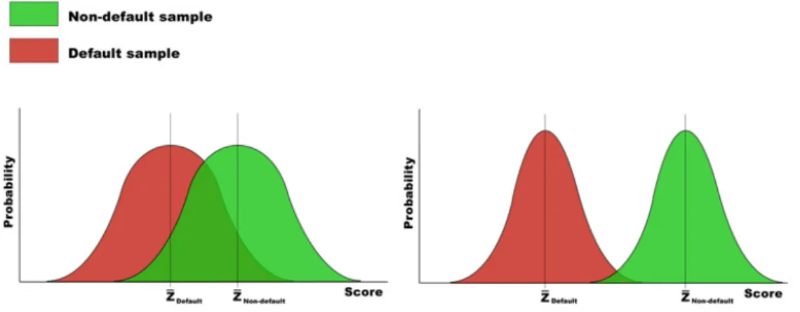
Z − − need not necessarily yield an optimal result. The reason is the variance of scores within each group. As can be seen in Figure 3.1, the graph to the left shows a distribution of scores of two groups and it becomes apparent that there is a large area where the two distributions overlap due to the high variance within each group. As a result, in order to optimize the discriminant function, the variance has to be included in the calculation. The term above achieves this. The numerator measures the variance between the default and non-default groups, also referred to as sum of squares between. By maximizing it, the centroids of the respective groups will drift further apart. The denominator, on the other hand, measures the variance of scores within each class and it is to be minimized. This is done by calculating the squared sum of deviations of individual scores Zig from
the group’s respective centroid Zg, also referred to as sum of squares within. Figure 3.1 below illustrates this process. The two distributions on the left are distributions of scores that are based on a random discriminant model. As long as the model operates with some intuition, for example higher profitability leads to a higher score, the model will probably be able to discriminate between good and bad loans to some extent. However, there will be an interval of scores that will include good and bad borrowers, i.e. the part where the distributions overlap. LDA lets the distributions drift further apart and makes them more skewed – the overlapping part is being minimized (the two distributions to the right).
Figure 3.1: The process of the linear discriminant analysis: distributions of the default and non-default sample based on a random discriminant model (left), distributions of the two samples after linear discriminant analysis has been applied (right).
Upon maximizing the above term, firms can be classified into one of the two groups of interest. This can be done by comparing the squared distances between the score for an observation and the centroids the two groups11:
(
)
2 2 g i ig Z Z D = −When this squared distance to the default group centroid is smaller than the squared distance to the non-default centroid, the firm will be classified as defaulted and vice-versa. Derived from these squared distances can be a critical value of Z*, for which if Zi < Z*, the firm will be assigned to the defaulted group.
For Zi > Z* it will be considered healthy.
It has to be pointed out, however, that it is almost impossible to obtain a discrimination function that perfectly discriminates between the two groups. A consequence of this is that there will always be score intervals where the distributions of the two groups overlap12. As a result, where the squared distances
between a score and the two centroids are very similar, there is a high probability of committing either a type 1 or a type 2 error. In the context of default prediction, a type 1 error is made when a bad customer is classified as good based on model output. A type 2 error occurs when a good customer is classified as bad by the model. A type 1 error will only occur in the case of Zi > Z*, while a type 2 error
only occurs when Zi < Z*.
Linear discriminant analysis has serious shortcomings. First of all, since the model is linear in nature, it assumes that there is a linear relationship between the independent variables and the eventual score. For example a 10% increase in the leverage ratio will always have the same effect on the score, irrespective of whether the leverage ratio is 5% or 75%. Intuitively, it is obvious that in the case of 5% leverage there will be a negative change in credit quality. However, it will not be as significant as in the latter case where a company loses virtually all equity. Another major problem is the weak interpretability of the score results. A score of, e.g. 2,04 does not indicate anything about the default probability. Hence,
11 See Backhaus et al. (2003).
while in terms of pure default and non-default classification discriminant analysis may be sufficient, in today’s banking world where the Basel II Accords require an estimation of default probabilities and the creation of several rating classes, discriminant analysis is of limited use. As a result, experts have turned their attention to Logit/Probit models, rendering the LDA obsolete for default prediction purposes.
3.2 Logit and Probit Models
Logit and Probit models are based on regressions and have one very useful property: the dependent variable can only take on values between 0 and 1. This is achieved through the use of the logit and probit functions. The logit function is the inverse of the logistic function. The logit of a probability is the logarithm of the odds of an event13, also referred to as the LogOdds. It has the following form:
⎟⎟ ⎠ ⎞ ⎜⎜ ⎝ ⎛ = p -1 p log logit(p)
The probit function, on the other hand, is the inverse cumulative distribution function associated with the standard normal distribution:
) ( )
(p 1 p
probit =Φ−
The advantage of the logit and probit is the fact that they transform the probability p into values ranging outside the zero and one boundary. This is a useful property since both Logit and Probit models are generalized linear models: the dependent variable is estimated from a linear combination of independent variables. Through the use of the logit and probit as link functions, the dependent variable is connected to the aforementioned linear combination of predictors in a manner that is desirable in a default prediction context, i.e. the output, p, is constrained between zero and one. Thus the results of default prediction models built on the basis of Logit and Probit models can be interpreted as default probabilities.
13 Odds are defined as
p p
− 1
At the heart of Logit models lies the logistic regression, which has the following form: e X b X b X b a p p n n + + + + = ⎟⎟ ⎠ ⎞ ⎜⎜ ⎝ ⎛ − 1 1 2 2K 1 ln
Again, a represents the constant, bn are the coefficients, Xn are the independent
variables and e is the error term. The left-hand term is the aforementioned logit. Through its use, the dependent variable, p, is constrained to values between zero and one. If Z is substituted for the entire right-hand side of the regression (i.e. Z is the score of the linear combination of dependent variables) then by reshuffling of the regression equation the default probability can be expressed as:
Z e p − + = 1 1
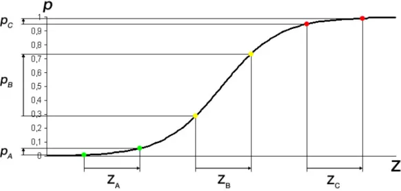
The relationship between the independent variables (Z) and the eventual score (p) corresponds more with reality and intuition, as illustrated with a small example. Suppose there is a simple logistic model which consists of only one input variable – the leverage ratio – and there are three firms (A, B and C). Firm A has the lowest leverage ratio while firm C has the highest leverage ratio. If all three firms increased their leverage ratio by the same amount of percentage points, their scores from the linear combination inputs would increase by the same amount. This can be seen in Figure 3.2 on the x-axis. When it comes to default probability, this increase will most likely have different effects, depending on the firm. For firms A and C, the increased leverage ratio will not result in very dramatic increases of PD. Firm A had a very small leverage ratio to start with and even after the increase the ratio would still be considered a healthy figure. Firm C already had a very high leverage ratio initially and hence a very high PD and thus the increased leverage only marginally affects the PD. On the other hand, firm B will be hurt most in terms of PD and subsequently the rating: while not too high at the start, the leverage ratio increased to levels where the firm will be considered substantially more risky. As a consequence, the PD has to increase more dramatically than in cases of firms A and C.
Figure 3.2: Relationship between independent variables (Z) and the eventual score (p) in a logistic regression.
The coefficients of the logit regression are obtained by means of maximum likelihood14 estimation. This estimation method is a statistical procedure that attempts to find the optimal combination of coefficients by maximizing the following likelihood function:
[
]
∏
= − − = n i y i y i i i p x x p LF 1 1 ) ( 1 ) (Here, p(xi) denotes the default probability of firm i as given by the logistic
regression equation and yi is a binary variable that takes on the value 1 if firm i
defaulted and 0 otherwise. The entire equation is essentially a product of the default probabilities of those companies in the dataset that defaulted and the survival probabilities (i.e. 1-p(xi)) of the dataset companies that did not default.
The maximized likelihood function is the one that maximizes the likelihood that the default prediction based on the logit regression is correct.
Probit models, on the other hand, utilize the probit link function in the generalized linear model and implicitly assume that the underlying variable is normally distributed (i.e. the score of the linear combination of factors is normally distributed). Formally, the probit regression function has the following form:
14 Likelihood is not to be confused with probability: while probability allows the inference of
probabilities of unknown outcomes based on known parameters, the concept of likelihood allows the inference of likelihoods of known outcomes for different values of the parameters.
( )
p =a+b X +b X +bnXn +e Φ− K 2 2 1 1 1The variables on the right hand side of the term are the same as in the logit model, while Φ−1
( )
p is the above mentioned probit. The relationship between the independent variables and the final score, which can also be interpreted as a default probability, is very similar to the relationship in the logit model depicted above.The utilization of the probit link function is less common than that of logit in default prediction. However, the choice of one of the two link functions does not have a substantial effect on the entire model development process – the steps in variable selection remain the same and so does the calibration. Moody’s KMV (2000) point out that in the past, logit was preferred due to computationally easier maximum likelihood estimation, an issue which has become irrelevant today. Even in professional literature on default prediction, there is no research into the matter of whether logit or probit delivers better results.
There is one assumption underlying these two models that should be kept in mind whenever one is designing a model using logit/probit: since they are both generalized linear models, both assume that the relationship between independents and the Logit/Probit (i.e. ln(p/(1-p) and Φ−1
( )
p respectively) is linear. However, with some financial variables, this is not always the case. A part of the chapter on variable selection will discuss this problem and possible solutions to this problem will be presented.3.3 Hazard models as an extension of traditional logit/probit models
In the recent past, some researchers have voiced their criticism of one particular characteristic of models based on either the discriminant analysis or logit/probit regressions: they do not specifically account for time. In order to overcome this deficiency, a small number of logit/probit models extended by inclusion of a hazard component which describes the default risk over time have been proposed. These models are referred to as hazard models and this section will briefly outline
their basic principles. Hazard models are rooted in survival analysis15, which is used in medicine to analyze the occurrence of death and time to death, such as the death rate of a population or the death rate past a certain age. Translated into credit risk modelling, it studies and analyzes the effect of time on the default probability of an exposure – in hazard models, the risk of bankruptcy changes with the passage of time.
At the heart of any hazard rate model in credit risk will be the modelling of the hazard rate, denoted in Cox & Oakes (1984) as:
) | ( ) (t dt =P t <T <t+dt T >t λ dt t) (
λ is the hazard rate16, t is a point in time, dt is one unit of time and T denotes the time of failure. In default prediction, T is the time of default. The hazard rate can be interpreted as the probability of default in the period between t and t + dt (i.e. per unit time) of a company given that it has survived until time t. Halling and Hayden (2004) present an example of modelling the hazard rate through the use of logistic regression. One starts with a normal logistic regression with the typical financial ratios as explanatory variables. This model serves as the basis for classifying firms into risky firms – firms that are, based on the data, in a critical situation and especially close to default – and risky firms. Risky and non-risky firms are then separated by a cut-off point in the estimated score – firms above a certain score will be included in a separate model.
The new model is basically also a logit model, but in this case it takes the time dimension into account. This is the hazard component, namely the number of periods that elapse between being assigned to the risky category and the possible default (default, of course, does not necessarily have to occur, even in the risky group). The model then takes on the following form:
e cD bX a yi = + i + it +
15 For more details on survival analysis, please see Cox & Oakes (1984) or Hosmer & Lemeshow
(1999).
16 The hazard rate is sometimes also referred to as instantaneous failure probability, conditional
The inclusion of the time component is done via the vector D. Dit is a dummy
variable that takes on the value of one for the particular firm-year observation that is t periods after the firm has been classified as risky. For example, in the firm-year observation of the firm i’s second period after being classified as risky, Di1
will be zero and Di2 will be one. This way the dependent variable is also
determined by the time spent in the group of risky firms and not just by accounting ratios. The independent variables of the vector X are chosen in the same fashion as those chosen for standard logit models.
3.4 Current state of modelling practice
The logistic functional form is currently dominating the field of default prediction in the absence of market data. The majority of internal rating models at banks use logistic regression to evaluate their corporate customers. Its main advantages lie in the fact that the output of such models is bound between zero and one. In addition, the relationship between the output and the independent variables is not linear and quite intuitive. Where linear discriminant analysis attempts to find a black and white solution by definition (i.e. classification into default and non-default), logit or probit models are more open towards producing a more diverse classification. In the past, where it would have been enough to find a tool that can make the decision whether to grant a loan or not, an LDA model would have been sufficient. However, with the emergence of the Basel II requirements and also with more risk-sensitive decision making tools such as RAROC17, logit/probit models are simply the more intuitive and better choice. Models that incorporate the hazard rate suffer from shortcomings which can be attributed to their non-existence in the IRB landscape. They are more sophisticated and as a result are more difficult to implement. Moreover, the use of such models in the corporate default prediction segment is a very new topic with very little research. Hence, there is no indication as to their track record in default prediction. As a consequence, the focus throughout the next chapters will be on logit/probit models since they represent the present state of the art.
17 Risk Adjusted Return on Capital (RAROC) is a commonly used risk-adjusted performance
4. Input variables
For a statistical default prediction model to work properly, i.e. to discriminate well between borrowers of different quality, the right combination of independent variables has to be found. Of course, one can estimate a regression with an arbitrarily chosen set of input variables and the significance of individual inputs varies with different datasets. As a result, the real challenge is to identify the first broad pool of “candidate” variables and then to find a procedure that narrows down the number of useful ratios to a few that will provide the best discrimination results.
Generally, input variables can be classified into two broad categories: quantitative data and qualitative data. While quantitative data utilizes financial figures taken from balance sheets and profit and loss statements, qualitative data attempts to capture information not reflected by hard numbers, such as management quality or market position. As opposed to quantitative data, the evaluation of qualitative data requires more input from loan specialists who also know the borrower. This process leans heavily on expert knowledge and is very similar to the development of scorecards for the evaluation of private individuals. Since the emphasis of this thesis is on statistical models which process financial data, only a broad overview of the issue of qualitative inputs will be given. In practice banks will have two separate models for the evaluation of quantitative data and qualitative data.
This chapter will deal with the topic of variable selection by first dealing with the choice of appropriate quantitative inputs and their combination into a model and presenting the quantitative variables selected into actual models from both research as well as practice. Finally, the topic of the inclusion of qualitative variables will be briefly discussed and an illustrative example of how quantitative and qualitative data are combined is given.
4.1 Quantitative inputs
In the absence of market data, the most viable input remains balance sheet as well as profit and loss statement data. As a result, most quantitative data will be in the form of financial ratios. The analysis of financial ratios is not new to economics as, for example, financial statement analysis is considered a basic tool to assess
the performance, profitability and general health of a company. The main advantage of financial ratios is the fact that they represent a fraction of two figures from the balance sheet. A single figure from the balance sheet is not very useful as there are vast differences between individual companies: an EBIT of €100.000 is good for a small firm but for a large corporation it practically equals zero profit. Setting this figure in relation to a size measure, such as total assets, enables the comparison of the small and large firm.
The amount of useful financial figures goes into the hundreds. As a result, analyzing each one is an inefficient and daunting task and providing an exhaustive list of all possible ratios does not make sense. For example, a simple profitability measure can be expressed in several variations depending on which figure one takes as the actual profit number – possibilities include Net Income, Ordinary Profit, EBIT and EBITDA. Nevertheless, in order to give an overview, most accounting data that is being used as an input into default prediction models, can be broadly categorized as follows:
1. Profitability ratios: these represent the most obvious group of ratios, as profitability is the most crucial indicator of a firm’s success. Higher profits are also reflected in higher equity and a profitable firm is much less likely to default on its obligations.
2. Leverage ratios: these ratios reflect the capital structure of a firm and indicate the degree to which it relies on external funding. Higher leverage translates into higher default probability as the buffer for losses – equity – is smaller and the threat of liquidation rises with a higher proportion of lenders.
3. Liquidity ratios: they measure the amount of a firm’s cash as well as resources that can be converted to cash very easily. The higher the liquidity, the higher a firm’s ability to repay obligations as they become due and to withstand unexpected shocks, and the lower the bankruptcy probability.
4. Coverage ratios: these ratios measure specifically the relation of performance and the amount of liabilities in the form of debt and interest payments. They are a combination of profitability and leverage.
5. Activity ratios: such ratios indicate the efficiency of the firm’s operations, often in terms of the turnover of a particular figure and as a result, these ratios are sometimes referred to as efficiency ratios.
6. Size: although size is not a ratio, it is a very important factor that has a substantial effect on the default probability. Presumably, larger firms have a bigger and more experienced and capable management team, they are more diversified and more diversification implies less volatility.
4.1.1 Identifying the relevant variables
The identification of the most strongly discriminating variables is the main step towards creating a default prediction model. In fact, Moody’s KMV (2000) state that “the selection of variables and their transformation are often the most important part of modelling default risk”. There is a certain amount of truth in that statement: while the regression itself can be accomplished fairly easily with today’s statistical software packages, a single set of clear, accurate rules and instructions to ensure that the modeller ends up with the best combination of factors and eventually an optimal model is non-existent. Instead, the variable selection is an iterative process that poses many challenges and demands some degree of creativity from the modeller.
Obviously, one has to start with a set of factors. However, as mentioned above, there are hundreds of potentially useful inputs. As a result, the analysis of all of them would be very time consuming and inefficient. Hence, one simply has to choose a smaller subset for evaluation. Altman (1968) described this process as a choice based on popularity in the literature, potential relevancy to the study as well as the inclusion of new ratios created by the study. This way, he ended up with 22 variables for the analysis. A closer look at other models also reveals that the first selection of variables is rather arbitrary and based on personal preference, as long as variables representing the categories described above (i.e. profitability, leverage, liquidity etc.) are considered. Fernandes (2005) starts the closer examination of the variables with 23 ratios, Altman (1977) uses a subset of 27 ratios, Altman (2005) starts with 17 variables. On the other hand, Moody’s KMV does not disclose how many factors were closely analyzed for the Riskcalc models.
Once an initial set of variables has been identified, the variables contained in that initial set have to be analyzed individually in the univariate analysis. In essence, the univariate analysis is a thorough screening of a variable in terms of its suitability for default prediction and consists of three steps:
a) Evaluation of the economic intuitiveness of the variable b) Evaluation of the discriminating power of the variable c) Removal of outliers
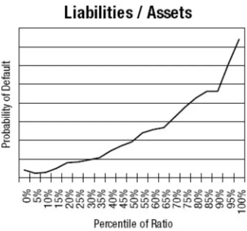
The first step is very straightforward – one has to have a clear idea of the expected relationship between the ratio in question and the default probability and the relationship should follow basic economic intuition. For instance, the ratio Equity/Total Assets is expected to have a negative relationship with the default probability. In other words, one expects the default probability to rise with a declining equity ratio – this is the general assumption and is very much in line with common sense. While the equity ratio will rarely run the risk of not having an intuitive relation to bankruptcy, there may be ratios that are more ambiguous. If a variable doesn’t show a clear and intuitive relationship to default, it should be dismissed from any further modeling considerations. Default frequency graphs are most widely used to graphically depict the relationship between an independent variable and bankruptcy. The following figure shows an example of a default frequency graph.
Figure 4.1: A sample default frequency graph. Source: Moody’s RiskCalc for Private Companies: UK.
To create a default frequency graph for a particular ratio (i.e. Liabilities/Assets in this case), all firm observations have to be sorted according to the size of the ratio
and then divided into equally sized groups in terms of numbers of observations so that each group corresponds to a different percentile range of the ratio in question. These groups are then plotted on the x-axis. In the figure above, each group contains five percent of the observations, however, the more observations are available the more groups can be created for this purpose. Finally, for each group the default frequency has to be calculated: the amount of defaults in that group divided by the total amount of firms in that group. This frequency is then plotted on the y-axis. The result is an easily observable relationship between the variable and the default probability.
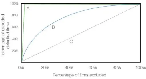
In order to test the discriminative power of individual variables, power curves, also referred to as Cumulative Accuracy Profile (CAP) plots, are usually constructed and from those the accuracy ratio can be calculated. The power curve is a graphical depiction of the ability of any variable or even model – power curves are also used to test the discriminative power of entire models18 – to
predict or influence the outcome of a binary event, i.e. default/non-default. Figure 4.2 shows an example of a typical power curve graph with three power curves.
Figure 4.2: Three sample power curves: perfectly discriminating variable (A), reasonably well discriminating variable (B), non-discriminating variable (C).
Usually a power curve has the shape of the B curve: if the B curve above showed the power curve of the Liabilities/Total Assets ratio, then the x-axis would contain the percentages of firms whose Liabilities ratio is worse than a given cut-off point.
In other words, as one moves from the worst value of the ratio to the best and at the same time from left to right on the x-axis, the percentage of firms will increase – the higher the cut-off ratio, the more firms will have a worse leverage. The y-axis plots, for any given cut-off point of the variable, the percentage of firms that actually defaulted and had a lower leverage ratio than that specified by the cut-off point. For example, curve B indicates that if the 20% of the worst performing firms in terms of leverage ratio are excluded from the dataset (x-axis), then approximately 60% of all defaulted firms from the dataset would be excluded. Curves A and C are extreme cases: curve A is a curve of a perfectly discriminating ratio – the kink is the point that separates the defaults from the non-defaults. As a result, if the population default rate is 3% and one excludes the worst 3% of the firms from the sample, based on that perfectly discriminating variable, all defaulted firms are identified. Curve C, on the other hand, is a power curve of a variable that has no discriminating power at all – for every cut-off, there is always the same proportion of defaults to non-defaults. Given these three exemplary curves, it is clear that the more northwesterly a curve lays, the higher its discriminating power.
The discriminating power can also be expressed in terms of a single number: the accuracy ratio19. In the example above, the accuracy ratio of the leverage ratio (curve B) would be calculated as:
(Area below curve B – Area below curve C) (Area below curve A – Area below curve C)
The accuracy ratio sets the discriminatory power of the studied variable in relation to the power of a perfectly discriminating variable.
Alternatively, the discriminating power of individual variables can be judged by estimating a regression for each variable individually. Based on these regressions, power curves are constructed in a similar way, the only difference being that instead of using the value of the ratio itself, one utilizes the result of the regression, i.e. the estimated univariate default probability associated with a particular variable.
In either case, the accuracy ratio is a popular tool to choose which variables will be considered in the regression model estimation. In terms of accuracy ratio, Fernandes (2005) only allows variables to enter multivariate analysis if they have an accuracy ratio of over 5%. Altman and Sabato (2006) use the two ratios from each ratio category with the highest accuracy ratio for the regression.
It has to be pointed out, that power curves and accuracy ratios for a single variable will be different across models and they do not represent a universal truth. Instead, the results one obtains from these discriminative power measures will depend on the sample being used in model development. For example, in samples containing firms where the leverage ratios are somewhat constant across the sample, the power curves for that ratio will have little information value and the accuracy ratios will be low. On the other hand in other samples, the ratio may very well have an effect on default and generate high accuracy ratios.
Finally, outliers, i.e. extremely high or low values pose a major threat and can bias the eventual result. Eliminating these values would lead to a reduction of data and thus it is advisable to restrict variables that are below the 1st percentile and above the 99th percentile to the 1st percentile value and 99th percentile value, respectively20. Altman and Sabato (2006) deal with the high variability of values in their SME model by logging all input variables and thus limiting the high range of variable values: estimating two logistic models using non-transformed ratios and logarithmically transformed ratios, the model with the logged inputs has an accuracy ratio of 87% compared to 75% of the other model.
4.1.2 Dealing with the non-linearity assumption in logit/probit models
While the process of identifying suitable financial data inputs will remain the same regardless of the functional form of the model, the process of transforming variables in order to deal with the non-linearity assumption between the independent variable and the logit/probit is an issue that only concerns models of that functional form. However, since the majority of current default prediction models are logistic, the possible solutions to this challenge will be discussed.
Altman and Sabato (2006) do not address this issue while Moody’s KMV (2000), OeNB (2004) and Fernandes (2005) do take this problem into account with different methods.
Non-linearity is dangerous, because in its presence the regression will underestimate the relationship between the independent variable and the dependent. A good example to illustrate this fact is sales growth21. In one interval, from negative sales growth to certain positive values of sales growth, the relationship to default probability (and thus to the Logit/Probit) is negative: the higher the sales growth, the lower the PD. Nevertheless from a certain point, when sales begin to grow excessively, the PD starts to increase. There are many reasons for this phenomenon: sometimes the firm’s expectations, based on the high growth, are too optimistic and it starts taking up too much debt financing. In addition, rapid growth presents numerous internal challenges to a company, such as expansion of the staff, new sales locations or a bigger management team. All these uncertainties cause the relationship to default become positive and higher sales growth will result in higher PDs. Eventually, the plot of the sales growth to the logit/probit will be a U-shaped curve, which is definitely not linear. A regression of this relationship will try to fit a straight line to depict the relation between the growth and the logit/probit. Since the actual relationship has the shape of a U, the fitted line will be rather flat with almost no slope. This is an indication of no or very weak relationship even though in reality there is a strong relationship.
Initially, the variables have to be checked for non-linearity. This can be accomplished by constructing graphs similar to the default frequency graphs where the x-axis remains the same and instead of plotting the empirical default probabilities, the empirical LogOdds (ln[p/(1-p)]) are plotted. The graph will indicate a non-linear relationship. It is also suggested to use a smoothing filter to smooth the data and reduce noise. The most widely used filter in credit risk literature is the Hodrick and Prescott22 filter which was developed to eliminate short-term fluctuations in macroeconomic time series. Using the filter, one obtains
21 Both Moody’s KMV (2000) and Halling & Hayden (2004) cite sales growth as a good example
of non-linearity between dependent and independent variable.
an even clearer visual representation of the relationship between a variable and the logit. A more statistical method to evaluate the linearity in logistic models is using the Box-Tidwell23 methodology: terms that multiply each independent variable with its natural logarithm are added to the regression, i.e. for each xi, there is also
an xiln(xi) term in the regression. If subsequent analysis shows that these terms are
significant, nonlinearity is present.
The Moody’s KMV (2000) solution to the nonlinearity problem is based on the univariate default frequency relationships. Instead of using non-transformed inputs into their probit model, they use the corresponding univariate default frequency for that particular variable. In essence, the inputs are derived directly from the smoothed default frequency graphs for each input variable. So for example, if firms with a leverage ratio of 20 percent had an empirical default rate of 0,5 percent, then 0,005 would be used as an input instead of 0,2. Moody’s KMV (2000) uses the univariate relationship between Net Income/Assets and default to demonstrate how the nonlinearity is captured – above a certain point this relationship is flat, i.e. no matter how high the profitability is, the default probability stays flat and does not decrease. As a result, when using the transformed inputs which reflect the univariate level of the default probability, the effect of a very high Net Income/Assets ratio will stay the same above a certain point. In a similar fashion, the OeNB (2004) bank analysis model24, which is based on a logistic regression, uses the smoothed (utilizing the Hodrick-Prescott Filter) univariate relationship between a variable and the empirical LogOdd as basis for the transformation. Afterwards the empirical LogOdds are used as inputs for variables that do not display a linear relationship with the LogOdd.
Another possibility to capture nonlinearity is by the use of polynomial expansion. For his logistic model, Fernandes (2005) applies the Fractional Polynomial Methodology developed by Royston and Altman (1994). In essence, this methodology attempts to find the best curve for a particular relationship between an independent and a dependent variable using polynomials that are limited to
23 See Box & Tidwell (1962) for further details.
24 This model is not further discussed in this thesis as it is aimed at default prediction of banks – a
segment which differs substantially from the corporate segment. Most IRB banks acknowledge this fact by creating separate models for banks and corporate customers.
only a small set of values, which should be sufficient to model the most common curve shapes. In a default prediction model with k explanatory variables, where variable X is suspected to be non-linear, it can be transformed into a fractional polynomial of the following form:
∑
= + − = m j j k j m X p H X 1 1 ) ( ) , ; ( β β φ where ⎪⎩ ⎪ ⎨ ⎧ = ≠ = − − − 1 1 1 ln ) ( j j j j j p j p p if X X H p p if X H jHere, m denotes the number of polynomial functions and p the power of function j. To illustrate, a model with three explanatory variables (i.e. k equals 3) – X, Y, Z – where only X is non-linear and one would use two polynomial functions (i.e. j=2) with p1=0.5 and p2=1 would have following form:
X X Z Y p p 4 3 2 1 0 1 ln ⎟⎟=β +β +β +β +β ⎠ ⎞ ⎜⎜ ⎝ ⎛ −
Based on their experience, Royston and Altman suggest restricting the possible powers to p = {-2, -1, -0.5, 0, 0.5, 1, 2, …, max(3, m)} and m=2 at most. The optimal values for p and m are found using an iterative process, described by Fernandes (2005). Firstly, a normal logit model is estimated with the non-linear variable treated as if it were linear. Afterwards, the first set of models with fractional polynomials is estimated: m is set to one and for each p from the above set a model is estimated. The model with the lowest deviance25 is then selected. Then the second set is estimated where m is set to two and for each combination of p a separate model is again estimated. The model with the lowest deviance is again selected. In the next step, the three estimated models (the regular logit model, the optimal m=1 and m=2 models) are compared via the likelihood ratio test. The optimal model is the one which has a significantly better fit than the
model with a lower degree of m and not a significantly worse fit than the model with a higher degree of m.
4.1.3. Final variable selection
Once the univariate analysis helps identify the most appropriate variables, the optimal model with the optimal combination of these pre-selected variables has to be found. As Moody’s KMV (2000) point out, from 20 independent variables one could create over one million possible models26. It is also not advisable to put all possible explanatory variables into the model, as it would then suffer from overfitting. An overfitted model produces very good prediction results when applied to the observations from within the sample used to estimate the model. However, it will have poor out-of-sample prediction results, i.e. when applied to completely new data it will have very low prediction reliability. The reason for this is multicollinearity: the presence of high correlation between some explanatory variables – for example, while the inclusion of all possible profitability measures in a model may reflect all aspects of profitability, the high correlation of these measures will cause serious instability when applied to out-of-sample data. A good way to eliminate this problem is to create a correlation matrix and check for pairs with very high correlation. After a model has been estimated, counter-intuitive signs of coefficients are hints of multicollinearity. Hence, a major goal lies in the achievement of parsimony for the model. In fact, the models discussed in this thesis do not have more than ten input ratios. Moody’s KMV (2000) mention many research papers and conclude that the optimal number of independent factors should be approximately seven. As a result, since it is suboptimal to use all variables from the univariate analysis and the combinations of possible models are numerous, automatic variable selection procedures, which are described below, have been devised.
For the commonly applied functional form of logit/probit27 models the forward selection, backward selection as well as stepwise regression selection procedures exist. Forward selection starts with the estimation of univariate models for each
26 If k denotes the number of candidate variables for possible inclusion, 2k – 1 models can be fitted.
27 For their Hazard model, Halling and Hayden (2004) use the stepwise regression selection
variable that was selected to be a potential candidate for inclusion. Of those models, the one with the most significant variable, found via the likelihood ratio test, is selected as the starting point for further testing. In the next step, one estimates all possible two-variable models – the most significant variable found previously is kept and another variable from the set of the remaining candidates is added. These two-variable models are then compared to the one-variable model selected in the first step based on their likelihood ratios. The two-variable model that has the highest likelihood ratio and also is significantly different28 from its one-variable counterpart then replaces the one-variable model. Further variables are added in the same way until the n+1 variable model is no longer significantly different from the n variable model identified one iteration before.
Backward elimination is the opposite: at first, the largest possible model that includes all candidate ratios is estimated. Subsequently, models where one variable is dropped are estimated. Using likelihood ratio tests, the least significant variable, i.e. the one with the lowest significance and where there is also not a significant difference between the full and the reduced model, can be eliminated. This procedure is continued until no more variables can be dropped because the n variable model is significantly different from the n-1 model.
Finally, stepwise regression is a combination of both forward selection and backward elimination. Stepwise regression starts with forward selection. At each iteration, once a variable has been added, all variables already in the model are checked for the possibility of elimination by means of the backward elimination. This process is continued until no additional variables can be added or removed. Ultimately, for a predefined significance level, these procedures should help the modeler find a final form for the logit/probit prediction model. However, even after the model has been estimated, the coefficients should be checked for plausibility, i.e. ratios with a negative relation to default (such as profitability ratios) should also have negative coefficients.
28 If it is not significantly different from the one-variable model, despite a higher likelihood ratio,
this implies that the additional variable does not have a significant influence on the dependent variable.
With respect to linear discriminant analysis, similar procedures to the ones described above for logit/probit models exist, the main criterion being the common statistical F-Test.
4.1.4 Variables selected into models
This subchapter will highlight the different statistical models and the inputs that make up those models. As already mentioned previously, they cover the main factors that predict default, however, the actual ratios and weights differ substantially.
i) Variables selected into logit/probit models Altman and Sabato’s SME model
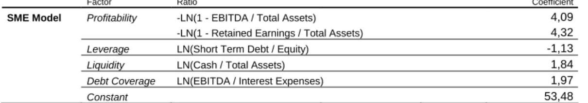
In their model, Altman and Sabato (2006) specifically tackle the default prediction problem for small and middle-sized firms in the United States. They make the case that banks should have different models for large corporates and SMEs: smaller firms have lower asset correlation but are in turn much riskier than their larger counterparts. As a result, the logistic model is based on a sample of firms whose asset size does not exceed $65 million. Eventually they present a set of five ratios that should be the most representative for SME default prediction in the United States. As already mentioned, the inputs were logged in order to constrain the large variability of the inputs.
Factor Ratio Coefficient
SME Model Profitability -LN(1 - EBITDA / Total Assets) 4,09
-LN(1 - Retained Earnings / Total Assets) 4,32
Leverage LN(Short Term Debt / Equity) -1,13
Liquidity LN(Cash / Total Assets) 1,84
Debt Coverage LN(EBITDA / Interest Expenses) 1,97
Constant 53,48
Table 4.1: input variables in Altman and Sabato’s SME model for the US.
Fernandes’ default prediction model
While not specifically focusing on small and medium-sized Portuguese firms, the dataset is dominated by SMEs, as they make up 95% of the dataset. Fernandes (2005) notes that the sample was chosen in a way as to approximate the overall structure of the Portuguese economy. An interesting aspect of his logistic default prediction model is the fact that the possibility of differentiation between different industries is studied. To achieve this, the dataset is split based on whether firms