Water Quality Factor Prediction Using Supervised Machine Learning

Portland State University

PDXScholar

REU Final Reports Research Experiences for Undergraduates on

Computational Modeling Serving the City

2018

Water Quality Factor Prediction Using Supervised Machine

Learning

Kathleen Joslyn

Portland State University, [email protected]

Let us know how access to this document benefits you.

Part of theEnvironmental Engineering Commons, and theHydraulic Engineering Commons

This Report is brought to you for free and open access. It has been accepted for inclusion in REU Final Reports by an authorized administrator of PDXScholar. For more information, please [email protected].

Citation Details

Joslyn, Kathleen, "Water Quality Factor Prediction Using Supervised Machine Learning" (2018).REU Final Reports. 6.

Water Quality Factor Prediction Using

Supervised Machine Learning

Kathleen Joslyn, Research Experience for Undergraduates (REU) at Portland State University

Abstract

The objective of this research is to explore prediction accuracy of water quality factors, with techniques and algorithms in machine learning consisting of a variation of support vector machines - Support Vector Regression (SVR) and the gradient boosting algorithm Extreme Gradient Boosting (XGBoost). Both the XGBoost and SVR algorithms were used to predict nine different factors with success rates ranging from 79% to 99%. Parameters of these algorithms were also explored to test the prediction accuracy levels of individual water quality factors. These parameters included normalizing the data, filling missing data points, and training and testing on a large set of data.

Intro

Supervised machine learning has shown itself to be an incredibly useful tool in many fields of study. Particularly in fields with an abundance of data. The United States Geological Survey in Portland, Oregon collects water quality data daily for a variety of factors. The sensor location used in this study collects data approximately every thirty minutes, this makes for a very large set of data. With this labeled data (labeled data is needed for supervised machine learning), a machine learning algorithm can be applied to predict different features. This has the potential to be incredibly useful for streamlining sensor calibration. Currently, data is gone through by hand to look for sensor malfunctions or oddities in the data.

Currently, water quality prediction using machine learning algorithms are a part of a slim field, with varying degrees of success. The purpose of this study is to assess two different algorithms, Support Vector Regression (SVR) and eXtreme Gradient Boosting (XGBoost), and their

performance in predicting nine different water quality factors. These factors are dissolved oxygen, pH balance, chlorophyll, temperature, specific conductivity, turbidity, cyanobacteria (blue-green algae), nitrate, and fluorescent dissolved oxygen matter (fDOM). Each factor is individually predicted in both algorithms using the eight other factors.

With the prediction of each of these water quality factors, it is proven that the accuracy of these algorithms could have the potential of many uses to the United States Geological Survey. With an implementation of these methods, it is possible to improve the quality of the water parameter data by changing the methods in which the sensors are monitored. Factor prediction using supervised machine learning is the beginning to a better monitoring system for aquatic ecosystems.

Background Work

Different Algorithms

A variety of machine learning algorithms were used in previous studies. These include Genetic Programming (GP, LGP), Support Vector Machines (and variations thereof –LS-SVM, and SVR), and Neural Networks (ANN, BP-NN, and GR-NN). No forms of gradient boosting were used. In this study, Support Vector Regression (SVR) and eXtreme Gradient Boosting

(XGBoost) are used to predict the nine separate factors.

Factor Prediction

Many of the papers studied for background work aimed at predicting individual water quality factors [1]-[5]. These included dissolved oxygen [1][2][3][6], fecal coliform [4], chlorophyll [5], and water temperature [6]. The papers studied for this research predicted these factors from a range of five to eighteen other water quality factors [1]-[6]. In contrast, this study is used to predict all nine factors and to study the relationship between these factors. Emphasis is put on exploring the outcomes of feature prediction and understanding how these predictions can be implemented in a useful way.

Data Used

Many of the studies used as background work used training and testing algorithms on relatively small data sets. A range of 132 to 2063 rows of data were used in these papers [1]-[6]. For this study, a total of 52,563 rows were used to train and test both the SVR algorithm as well as the XGBoost algorithm. The training and testing data were also split in different ways. Most of the testing and training data were either split 75/25 [2][4] or 80/20 [1][3]. In contrast, this study split training and testing data at 90% and 10% respectively.

Methods

The algorithms that are used to test water quality factors consist of a type of Support Vector Machine (SVM) called Support Vector Regression (SVR) and the gradient boosting algorithm XGBoost (eXtreme Gradient Boosting). The algorithms were implemented using Python in Jupyter Notebook with libraries such as SciKit-Learn, Pandas, NumPy and Seaborn. Each

algorithm trained and tested on a data set from the United States Geological Survey consisting of three years of data from July 20th_{, 2015 to July 19}th_{, 2018. Each algorithm handled 52,563 rows}

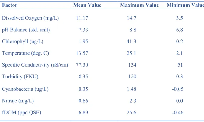
and nine columns for a total of 473,067 data points. Any missing values were filled with the mean values of their individual column. Each factor’s maximum, minimum and mean value is listed in figure 1 below.

Figure 1: Water quality factor’s mean, maximum, and minimum values.

Factor Mean Value Maximum Value Minimum Value

Dissolved Oxygen (mg/L) 11.17 14.7 3.5

pH Balance (std. unit) 7.33 8.8 6.8

Chlorophyll (ug/L) 1.95 41.3 0.2

Temperature (deg. C) 13.57 25.1 2.1

Specific Conductivity (uS/cm) 77.30 134 51

Turbidity (FNU) 8.35 120 0.3

Cyanobacteria (ug/L) 0.35 1.48 -0.05

Nitrate (mg/L) 0.66 2.3 0.0

fDOM (ppd QSE) 6.89 25.6 -0.46

Out of 13 total factors that are collected from the USGS sensor, nine factors were chosen to train and test the model. Factors were chosen by considering the timeline of when data began being collected. Much of USGS data varied in terms of quality and frequency of collection. Those factors that were cut from consideration had either been only recently collected (within the last year) or were irrelevant to the prediction of any of the nine other factors.

The dataset was downloaded from the USGS site. The sensor data is collected from the Morrison Bridge in Portland, Oregon in the United States. Each data point is collected at thirty-minute intervals every day. Missing data was initially a problem with early data collection in July and August of 2015, this was taken care of by filling in missing data with the mean value of the individual columns.

The main goal was to predict dissolved oxygen concentration; however, prediction of the other factors was also considered. Each prediction accuracy score is measured ten times, then the highest score, lowest score and the mean values for each factor prediction are considered. Each factor had varying degrees of success, with temperature having the highest prediction accuracy in both SVR and XGBoost. Dissolved oxygen was also successful with a 98.35% best prediction in SVR. The rest of the factors ranged in prediction accuracy from 77% to 99%. Most stayed within one or two degrees with minimal variance.

The SVR algorithm ran at approximately two minutes for each prediction. While slower than XGBoost (where XGBoost ran at approximately 10 to 15 seconds to predict each factor), it tended to have more accurate prediction rates for nearly all factors, especially for dissolved oxygen.

Trial and Error

Many techniques were tried when testing each factor. Most of the experiments were done on dissolved oxygen prediction. The first run of the SVR algorithm was done on a small data set, no more than 139 rows were used. The first run of SVR resulted in a negative prediction percentage (in SVR, a negative percentage value means an extremely poor regression fit). The second attempt was made after dropping all but four of the total parameters.

This lead to an increase in the amount of data being used for prediction, which raised the accuracy prediction. However, when reviewing the data by hand, it was found that there were many missing values for each column. To better the SVR prediction accuracy, each missing data point was filled with the individual column mean values. Each mean value for the factors is listed in figure 1. After filling each missing point, the SVR algorithm was run once more to predict dissolved oxygen data points.

It was found that after addressing missing data, and pulling large amounts of data from USGS, the SVR algorithm produced a range of 90 to 93% prediction accuracy rating for dissolved oxygen. After this acceptable run, more data was collected in the attempt to up the accuracy. This allowed the SVR model to perform within the 97 to 98% range to predict dissolved oxygen levels. Once a method was established for the SVR algorithm, the same method was applied to the XGBoost algorithm with the same data set.

Normalizing the data was also attempted to better the prediction accuracy of both SVR as well as XGBoost. Three normalizing techniques were attempted in both algorithms. The first and

foremost attempt was using the normalizing function in SciKit-Learn. By using.norm(), the data would be normalized in between a specified range, in this example, data was normalized from -1 to 1. However, this produced a negative prediction percentage. The second attempt at

normalizing the data was by using a simple formula (where X represents all nine columns and 52,563 rows, and N is the normalized outcome):

𝑁 = 𝑋$ − 𝑋&$' 𝑋_&()− 𝑋_&$'

The simple formula allowed for normalization to be condensed in between 0 and 1. This normalization technique produced positive prediction ratings for dissolved oxygen that had an average of 92.60%. While less than the prediction accuracy of the untreated data, the SVR algorithm ran much quicker over the normalized data.

Results

The initial goal was to predict dissolved oxygen within a reasonable percentage. However, the other eight factors were also predicted due to the ease of testing each factor. The results varied based on the algorithm used as well as the factor being predicted.

SVR

The SVR algorithm was able to predict most factors within a reasonable range. Out of the nine factors tested, the lowest performance had a mean prediction accuracy of 81.45% for turbidity, seen in the figure below in figure 2.

The best performance had a mean prediction accuracy of 98.43% for temperature with dissolved oxygen following close behind with an average of 97.89%, this is visualized in the graphs below.

Figure 3

Temperature prediction using SVR. Many points are predicted accurately with only some spikes being harder to predict.

Figure 2

Turbidity prediction using SVR. Blue is actual value, orange is predicted value. SVR had trouble predicting the spikes in turbidity measurements.

While the SVR algorithm produced prediction accuracies at 79.32% and above, the tradeoff came in the amount of time it took to run each prediction. Dissolved oxygen prediction had a run-time of approximately two and half minutes each time the program was run. While some factor predictions took over three minutes to produce results. The chart below states the predication accuracy scores for each factor’s mean prediction as well as the highest and lowest prediction accuracies in the SVR algorithm.

Figure 5: SVR Factor Prediction Accuracy

Factor Mean Prediction Highest Prediction Lowest Prediction

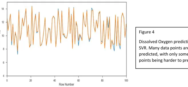
Dissolved Oxygen 97.89% 98.35% 97.56% pH Balance 86.54% 87.46% 85.57% Chlorophyll 88.20% 89.72% 86.27% Temperature 98.43% 98.80% 98.18% Specific Conductivity 87.84% 89.46% 86.87% Turbidity 81.45% 83.67% 79.32% Cyanobacteria 88.52% 88.80% 88.11% Nitrate 94.69% 94.93% 94.43% fDOM 93.57% 94.34% 92.68% Figure 4

Dissolved Oxygen prediction using SVR. Many data points are accurately predicted, with only some of the low points being harder to predict.

XGBoost

XGBoost was able to predict each factor above an 80% accuracy score. The lowest mean

prediction accuracy was an 81.64% for pH balance, with the highest mean prediction accuracy at 98.49% for temperature. Unlike turbidity prediction with SVR, where there was a discernable pattern for not predicting as well as the other factors, pH balance in XGBoost had no real pattern, with a relatively poor prediction in general. The highest prediction values were for temperature, with an average of 98.49%, cyanobacteria with an average of 94.43%, and dissolved oxygen with a prediction accuracy of 94.46%. XGBoost did undoubtably well for temperature prediction, but other factors were much lower in relation to the SVR algorithm. However, runtime for XGBoost is very fast, with each parameter taking a matter of seconds to output a prediction percentage. The chart below states each factor’s mean accuracy scores as well as the highest and lowest prediction accuracies of each individual factor.

Figure 6: XGBoost Factor Prediction Accuracy

Factor Mean Prediction Highest Prediction Lowest Prediction

Dissolved Oxygen 94.46% 94.71% 94.14% pH Balance 81.64% 82.86% 80.42% Chlorophyll 87.94% 88.69% 86.73% Temperature 98.49% 98.57% 98.36% Specific Conductivity 88.57% 88.96% 87.60% Turbidity 93.76% 94.93% 91.95% Cyanobacteria 94.93% 94.86% 94.09% Nitrate 91.60% 91.97% 91.28% fDOM 88.31% 88.86% 87.69%

Relationships Between Factors

To analyze the results further, the factor correlations were calculated to better understand the relationships between the water quality factors. Correlations were calculated in XGBoost and verified in SVR.

Dissolved Oxygen Correlations

Factor Correlation Percentage Cyanobacteria 88.32%

Nitrate 77.95%

fDOM 68.66%

Turbidity 55.67%

Turbidity Correlations

Factor Correlation Percentage Nitrate 67.21%

fDOM 60.66% Dissolved Oxygen 55.67% Cyanobacteria 55.24%

Temperature Correlations

Factor Correlation Percentage Specific Cond. 58.99%

Chlorophyll 53.29% pH Balance 49.79%

Chlorophyll Correlations

Factor Correlation Percentage Dissolved Oxygen 59.01%

Temperature 53.29% Specific Cond. 35.46%

fDOM Correlations

Factor Correlation Percentage Nitrate 77.02%

Dissolved Oxygen 68.66% Cyanobacteria 63.60% Turbidity 60.66%

Nitrate

Factor Correlation Percentage Dissolved Oxygen 77.95%

fDOM 77.02% Cyanobacteria 74.48% Turbidity 67.21%

Specific Cond. Correlations

Factor Correlation Percentage pH Balance 59.60%

Temperature 58.99% Chlorophyll 35.46%

pH Balance Correlations

Factor Correlation Percentage Specific Cond. 59.60%

Chlorophyll 59.01% Temperature 49.79%

Cyanobacteria

Factor Correlation Percentage Dissolved Oxygen 88.32%

Nitrate 77.48%

fDOM 63.60%

Turbidity 55.24%

Figure 7

Discussion

Both SVR and XGBoost performed well in one or more factor prediction scenarios. The tradeoff ultimately is the runtime for the two algorithms. While XGBoost is fast, its prediction rates fall short of the SVR algorithm. The most satisfactory predictions are above 95%, where SVR has two factors within that percentile, while XGBoost has one within that percentile. A still acceptable level of 90% to <95% was also recorded in both SVR and XGBoost. In this area, XGBoost performed better with four of the nine factors being within that percentile, while SVR had two. The most common performance percentages were within the 85% to <90%. In this range, SVR had four factors that were predicted within this range and XGBoost had three factors in this range. Both SVR and XGBoost had one factor that had an accuracy prediction below an 85%.

The best outcomes of both algorithms were the prediction of temperature. SVR also predicted dissolved oxygen with good results. Some factors varied by more than 5% between the two algorithms, the most severe difference is seen in the prediction of turbidity, while cyanobacteria and fDOM also had larger gaps in factor prediction. In general, out of the three factors that varied the most, XGBoost favored the more accurate predictions in turbidity and cyanobacteria while SVR had a better accuracy prediction for fDOM.

Each algorithm had its own strength. XGBoost performs fast, and overall had good, but not great results for many of the water quality factors. SVR was much slower than XGBoost but boasted great prediction accuracy for two of the nine factors. Both algorithms had decent performance in most of the factors. It would be a matter of adjusting parameters within both algorithms to see what, if any, of the factors could be better predicted.

Future work

Preliminary runs were tested on “pseudo forecasting” for dissolved oxygen prediction. The goal will be to test the window in which a factor can be reliably predicted. If a factor can be predicted accurately and with a reasonable amount of data, then that can be applied as a warning system for the sensors that collect this data. Currently, every piece of data is gone through by hand. Problems and malfunctions with the sensors are then dealt with if the data is missing or if the data does not fit normal patterns. Any anomalies are handled by either using accurate data from other close by sensors or dropping the data altogether. If the algorithms tested in this study can be utilized to predict future water quality factor values, then manually going through the data would not be needed. Instead, if the algorithms can accurately predict a data point, and the actual data point is way off from the predicted value, then an alert can be tripped to check the sensor for malfunctions or problems in the sensor’s environment. This would be incredibly useful to the USGS in terms of saving time and money.

Conclusion

Supervised machine learning is useful in many ways and in many fields. The power of prediction and anomaly detection have proven to be a huge influence on environmental studies. Water quality is hugely important to the ecosystem, and the Willamette River is a lifeblood to Portland. It is crucial to keep the water ecosystem healthy. The sensors that the USGS upkeep play an important role in monitoring water quality. With the current system, many man hours are spent analyzing the data by hand. With the utilization of machine learning algorithms such as SVR and XGBoost, it is possible to predict these water quality factors with percentages above 80%. With prediction accuracies as high as 98.49%, it can be shown that water quality factors can be predicted with accuracies above 80% and up to 98.50%. With this fact established, work can be continued to reduce the amount of time and money spent on manually going through sensor data.

References

[1] S. Malek, M. Mosleh, and S. M. Syed, “Dissolved Oxygen Prediction Using Support Vector Machine,” vol. 8, no. 1, p. 5, 2014.

[2] E. Olyaie, H. Zare Abyaneh, and A. Danandeh Mehr, “A comparative analysis among computational intelligence techniques for dissolved oxygen prediction in Delaware River,”

Geoscience Frontiers, vol. 8, no. 3, pp. 517–527, May 2017.

[3] X. Ji, X. Shang, R. A. Dahlgren, and M. Zhang, “Prediction of dissolved oxygen

concentration in hypoxic river systems using support vector machine: a case study of Wen-Rui Tang River, China,” Environ Sci Pollut Res, vol. 24, no. 19, pp. 16062–16076, Jul. 2017. [4] M. S. Jadhav, K. C. Khare, and A. S. Warke, “Water Quality Prediction of Gangapur

Reservoir (India) Using LS-SVM and Genetic Programming,” Lakes & Reservoirs: Science, Policy and Management for Sustainable Use, vol. 20, no. 4, pp. 275–284.

[5] Y. Park, K. H. Cho, J. Park, S. M. Cha, and J. H. Kim, “Development of early-warning protocol for predicting chlorophyll-a concentration using machine learning models in

freshwater and estuarine reservoirs, Korea,” Science of The Total Environment, vol. 502, pp. 31–41, Jan. 2015.

[6] S. Liu, H. Tai, Q. Ding, D. Li, L. Xu, and Y. Wei, “A hybrid approach of support vector regression with genetic algorithm optimization for aquaculture water quality prediction,”