Full Terms & Conditions of access and use can be found at
http://www.tandfonline.com/action/journalInformation?journalCode=tgnh20
Geomatics, Natural Hazards and Risk
ISSN: 1947-5705 (Print) 1947-5713 (Online) Journal homepage: http://www.tandfonline.com/loi/tgnh20
Ensemble machine-learning-based geospatial
approach for flood risk assessment using
multi-sensor remote-sensing data and GIS
Hossein Mojaddadi, Biswajeet Pradhan, Haleh Nampak, Noordin Ahmad &
Abdul Halim bin Ghazali
To cite this article: Hossein Mojaddadi, Biswajeet Pradhan, Haleh Nampak, Noordin Ahmad & Abdul Halim bin Ghazali (2017) Ensemble machine-learning-based geospatial approach for flood risk assessment using multi-sensor remote-sensing data and GIS, Geomatics, Natural Hazards and Risk, 8:2, 1080-1102, DOI: 10.1080/19475705.2017.1294113
To link to this article: https://doi.org/10.1080/19475705.2017.1294113
© 2017 The Author(s). Published by Informa UK Limited, trading as Taylor & Francis Group
Published online: 01 Mar 2017.
Submit your article to this journal Article views: 1109
View related articles View Crossmark data
Ensemble machine-learning-based geospatial approach for
fl
ood
risk assessment using multi-sensor remote-sensing data and GIS
Hossein Mojaddadia, Biswajeet Pradhan a,b, Haleh Nampaka, Noordin Ahmadaand Abdul Halim bin GhazaliaaDepartment of Civil Engineering, Faculty of Engineering, University Putra Malaysia, Serdang, Selangor, Malaysia; bDepartment of Energy and Mineral Resources Engineering, Sejong University, Seoul, Republic of Korea
ARTICLE HISTORY
Received 2 November 2016 Accepted 8 February 2017
ABSTRACT
In this paper, an ensemble method, which demonstrated efficiency in GIS basedflood modeling, was used to createflood probability indices for the Damansara River catchment in Malaysia. To estimateflood probability, the frequency ratio (FR) approach was combined with support vector machine (SVM) using a radial basis function kernel. Thirteen flood conditioning parameters, namely, altitude, aspect, slope, curvature, stream power index, topographic wetness index, sediment transport index, topographic roughness index, distance from river, geology, soil, surface runoff, and land use/cover (LULC), were selected. Each class of conditioning factor was weighted using the FR approach and entered as input for SVM modeling to optimize all the parameters. Theflood hazard map was produced by combining theflood probability map withflood-triggering factors such as; averaged daily rainfall and flood inundation depth. Subsequently, the hydraulic 2D high-resolution sub-grid model (HRS) was applied to estimate theflood inundation depth. Furthermore, vulnerability weights were assigned to each element at risk based on their importance. Finally
flood risk map was generated. The results of this research demonstrated that the proposed approach would be effective forflood risk management in the study area along the expressway and could be easily replicated in other areas.
KEYWORDS
Flood risk assessment; vulnerability; hazard; GIS; SVM; 2D HRS; inundation; remote sensing; Malaysia
1. Introduction
Flood events are typically regarded to be the most common natural disaster worldwide (Stefanidis & Stathis2013). Hence,flood risk management is an important challenge in many cities. Rapid urbani-zation, population growth, economic development, and climate change will increase the magnitude of this challenge (Huong & Pathirana2013). Considerable and irreparable damages to farmlands, transportation, bridges, and many other aspects of urban infrastructure prove the urgent require-ment forflood control and prevention (Tehrany et al.2014; Pradhan et al.2014).
Flood risk analysis and risk mitigation are two components offlood risk management. Flood risk analysis aims to investigate where the risk offlood occurrence is unacceptably high and where risk mitigation actions are required. Therefore, comprehensiveflood risk analysis by detecting hazardous and risky areas is an essential part of risk management to estimate the amount of damages that can occur because offlooding (Meyer et al.,2008).
CONTACT Biswajeet Pradhan [email protected]; [email protected]
© 2017 The Author(s). Published by Informa UK Limited, trading as Taylor & Francis Group
This is an Open Access article distributed under the terms of the Creative Commons Attribution License (http://creativecommons.org/licenses/by/4.0/), which permits unrestricted use, distribution, and reproduction in any medium, provided the original work is properly cited.
VOL. 8, NO. 2, 1080–1102
The recent improvements in the efficiency of remote sensing (RS) and geographic information system (GIS) technologies have initiated a revolution in hydrology, particularly inflood manage-ment, which can fulfil all the requirements forflood prediction, preparation, prevention, and dam-age assessment (Tehrany, Pradhan, & Jebur 2013). Among different GIS-based flood models presented in the literature, artificial neural networks (Kia et al., 2011), frequency ratio (FR) (Lee et al. 2012), logistic regression (Pradhan 2010), adaptive network-based fuzzy inference system (Chau et al.2005), multi-layered feed forward network (Kar et al.,2015), decision trees (Tingsan-chali & Karim2010; Merz et al.2013; Tehrany et al.2013), and support vector machines (SVMs) (Zhou et al.2013; Tehrany et al.2014) are the most widespread techniques that utilize RS and GIS tools. Althoughflood forecasting and prediction models are available, the accuracy offlood predic-tion maps remains a critical issue. Inflood modelling, a high accuracy forflood prediction mapping should be achieved, and thus, new and efficient models should be explored to increase the accuracy.
Flood risk can be expressed as a combination of hazard and vulnerability (Apel et al.,2008; Inter-governmental Panel on Climate Change 2014; Vojinovic & Abbott 2012). In particular, risk is a mathematical expectation of the vulnerability (consequence) function. Flood probabilities are deter-mined to produce flood hazard maps. Hydraulic models may result in uncertainties because they require complete and sufficient hydrological data (Horritt2006); therefore, using RS data and GIS-based models can be considered a complementary approach toflood modelling (Lecca et al.2011).
The current research aims to determine theflood risk level in a study area that is affected by annualflooding. An appropriateflood prediction assessment is required in the study area to prevent incurring additional cost in the future because of the proximity of the area to an expressway, whose construction has already reached an exorbitant cost. As the main components of risk assessment,
flood hazard and vulnerability indices were developed in this research through an accurate RS data and GIS-based ensemble model. The result of this research will provide an overall and accurate pic-ture offlood vulnerable areas using detailed information to protect lives and properties along the New Klang Valley Expressway (NKVE) in case offlood events by implementing appropriate disaster management techniques.
2. Study area
Severeflood events that occurred during the past decades in Malaysia have seriously threatened its population, economy, and environment. Thisfinding is evident from the increase in the amount of damages caused by a series of extreme floods in Malaysia over the last 50 years (Tehrany et al.
2013). One of the huge economic disadvantages offlooding is damages to highways. Thus, the Dam-ansara River catchment along NKVE, which is seriously affected byflooding, was selected as the study area for a detailedflood hazard and risk analysis and modelling. The Damansara River catch-ment is located beside Kampung Baru Subang in Selangor, Malaysia. The study area is situated at 38ʹ45.600 latitude and 10132ʹ27.2400 longitude. Damansara River stretches from Sungai Buloh to Shah Alam. The location and boundary of the study area were accurately delineated using a digital elevation model (DEM), as shown inFigure 1.
As shown inTable 1, information regarding the hydro-geomorphological characteristics of the study area, such as basin slope, area, and length, was calculated using GIS Spatial Analyst tools. First, aflow direction map was extracted from the DEM from which the watershed boundary was delin-eated using hydrology basin tool. Next, main river length and upstream distance were calculated by using theflow length option in hydrology toolbox. Next, basin slope was calculated by using surface raster-based tool in percentage. Then using Zonal statistical analysis, average value was extracted. The total area of the Damansara River catchment was estimated at approximately 116.9 km2, while the length of Damansara River was 22.22 km.Figure 2shows the Damansara River catchment with itsflow direction over the study area.
3. Data used
3.1. Flood inventory
To evaluateflood risk in an area, analysing records of pastflood events is essential (Manandhar
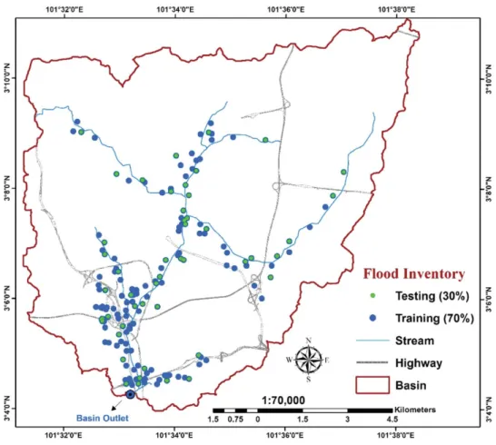
2010). Therefore, an inventory map is considered the most essential factor for predicting future disaster occurrence; such map can represent single or multiple events in a specific area (Tien Bui et al.2012a). In the current research, aflood inventory map was primarily created by mapping the singleflood locations where the exceed water has been running by using thefield measurement and surveying. The preparedflood inventory map comprised 110fluvial-flooded events, when collected from 2010 to 2015 over Damansara river catchment.
Figure 1.Location map of the study area.
Table 1.Hydro-geomorphological details for Damansara river catchment.
Hydrological characteristics Value
Basin slope (D) 0.07
Maximumflow distance (m) 22222.66 Maxflow distance slope (D) 0.01 Stream centroid to outlet (m) 8426.41 Area facing south 53% Area facing north 47% Maximum stream length (m) 21473.58 Maximum stream slope (D) 0.00 Basin length (m) 15625.50 Basin shape factor 2.09 Basin perimeter (m) 71440.35 Basin average elevation (m) 37.86
CENTROID X 397595.17
CENTROID Y 346340.79
Basin LA county lateral 65.00 Basin LA county basin hydrograph 2.00 Basin area (km2) 116.90
Theflood inventory map was divided into 70% training area and 30% validation area (Tunusluoglu et al.,2007), as shown inFigure 3. The trainingflood locations (77 out of 110 points) were randomly selected. Then, theflood layer, which was considered a dependent factor, was constructed. Theflood layer was developed using two sets of value, namely, 0 and 1. 0 indicates the absence offlood events, whereas 1 indicates the presence offlood events across an area. Similarly, an equal number of points (77 out of 110) were selected as non-flooded areas to achieve a value of 0. Flooding could not occur in high-elevation regions such as hills; hence, non-flooded areas were randomly selected from these loca-tions. The remainingflood locations (33 points) were utilized for model validation.
3.2. Flood-conditioning factors
In recent years, many spatial methods have been proposed by researchers for mappingflood hazard and risk zones to spatially delineateflood-prone areas. Building aflood hazard assessment model requires a set offlood-related parameters (Tehrany et al.2014). The precision and quality of meth-ods can be affected by the manner in which an accurate GIS database is used. Therefore,fl ood-con-ditioning factors should be optimized to enhance results.
Theflood-conditioning factor data set used in this research consisted of 13 factors, namely, alti-tude, aspect, slope, curvature, stream power index (SPI), topographic wetness index (TWI), sedi-ment transport index (STI), topographic roughness index (TRI), distance from river, soil, geology, surface runoff, and land use/cover (LULC). In this research, the cell of each conditioning factor was resized to 5 m£5 m, and the grid of the Damansara River catchment was constructed with 2650 columns and 2623 rows.
3.2.1. DEM-derived factors
The DEM was built using Interferometric Synthetic Aperture Radar (IFSAR) images with a pixel size of 5 m£5 m which was captured in 2014. Consequently, all topographical map factors, such as alti-tude, slope, aspect, curvature, STI, SPI, TWI, and TRI, were derived from the DEM.
One of the most influential parameters in flood studies is elevation (Figure 4(a)), and a flood event occurring in highly elevated areas is nearly impossible (Botzen et al.2012). Waterflows from highly elevated terrains toward lower regions, and thus, the probability offlood occurrence is natu-rally higher in flat regions. Moreover, topographical parameters that are directly affected byflow extent and runoff speed have important roles inflood occurrence (Kia et al.2011). Each topographi-cal parameter related toflood occurrence in any area is extracted directly from the DEM. Thus, a highly precise DEM is essential (Pradhan2009).
Slope is another topographical factor that is regarded as an important parameter in hydrology (Tehrany et al.2013) because of its effect in producing runoff in an area and its influence on runoff speed. An increase in slope degree decreases time for surface infiltration; subsequently, a huge amount of water enters the drainage network and causes aflood event (Figure 4(b)). Slope aspect commonly refers to the horizontal direction toward which the slope of a mountain is facing. An aspect map also plays a significant role in assessing the slope stability of a local terrain, depending on the type of slope face (Figure 4(c)). Curvature, which is split into three classes (convex, concave, andflat regions), is another influential parameter inflood occurrence (Figure 4(d)).
SPI and TWI are water-related parameters that are calculated using the following formulas (Gok-ceoglu et al.2005):
SPI ¼ As tanb; (1)
TWI ¼ lnðAs=tanbÞ; (2)
where Asis the specific catchment area (m2m¡1), andb is the local slope gradient measured in degree.
The SPI factor indicates the erosive power of waterflow (Figure 4(e)). TWI represents the effect of topography on runoff generation and the amount offlow accumulation at any location in the river catchment (Gokceoglu et al.2005), as shown inFigure 4(f).
The accuracy of a topographic index can be estimated with regard to grid spacing and terrain roughness by comparing the topographic index surface with respect to reference data. TRI, as one of the morphological parameters widely used inflood analysis, is calculated using the following equation: TRI ¼pffiffiffiffiffiffiffiffiffiffiffiffiffiffiffiffiffiffiffiffiffiffiffiffiffiffiffiffiffiffiffiffiffiffiffiffiffiffiAbs maxð 2min2Þ; (3)
Figure 4.Flood-conditioning factors: (a) altitude, (b) slope, (c) aspect, (d) curvature, (e) SPI, (f) TWI, (g) TRI, (h) STI, (i) distance from river, (j) soil, (k) geology, and (l) surface runoff.
where max and min are largest and smallest values of the cells in the nine rectangular neighbourhoods of altitude (Figure 4(g)).
The erosion and deposition processes are characterized using STI (Figure 4(h)), as presented in the following equation (Moore & Wilson1992):
STI¼ ðmþ1Þ ðAs=22:13ÞmsinðB=0:0896Þn; (4) whereAsis the specific catchment area (i.e., the upslope contributing area per unit contour length) estimated using one of the available flow accumulation algorithms in the Hydrology toolbox of Figure 4.(Continued)
ArcGIS, andBis the local slope gradient in degrees. The contributing area exponent,m, is generally set to 0.4, whereas the slope exponent,n, is generally set to 1.4.
3.2.2. Distance from river
Flood occurrences in the study area are frequent along the stream. Thus, distance from the river was considered another geomorphology-related conditioning factor. Subsequently, a distance from the river map was generated because the streams would disrupt the stability of the slopes either by toe undercutting or by saturating parts of the materials lying within the water level of stream ways. Dis-tance from a river is represented by the proximity of rivers and drainages in an area. In the current research, a distance from the river map was developed from the vector map of rivers using Euclidean distance in ArcGIS 10.3 software. Then, the resulting shapefile was converted into a 5 m raster and divided into 10 classes using the quantile method (Figure 4(i)).
3.2.3. Lithological and soil type
Lithological and soil maps are highly important parameters infinding sensitive areas prone tofl ood-ing. Soil type directly affects the drainage process because of soil characteristics, such as texture, per-meability degree, and structure. The study area is characterized by seven soil types. The spatial distribution of each soil type is shown inFigure 4(j). Lithological information regarding the perme-ability of rocks is also required inflood hazard assessment. Therefore, soil types and lithology are vital for conducting analysis in this research.Figure 4(k) presents the geology map, which shows that three types of lithology cover the study area. The majority of the eastern section of the study area is covered by acid intrusives, whereas the western section is covered by phyllite, slate, shale, and sandstone. 3.2.4. Surface runoff
Soil capacity is fully saturated by water throughout the land, and water flow exceeds the limits required for surface runoff (Figure 4(l)). This parameter was estimated using an empirical equation called the Soil Conservation Service curve number (SCS-CN) method,
Q ¼ðP0:2sÞ
Pþ0:8s (5)
S ¼1000
CN 10; (6)
whereQis the direct runoff (mm),Pis the accumulated rainfall (mm),Sis the potential maximum soil retention (mm), andCNis the curve number.
3.2.5. LULC
Another primary related factor that strongly contributes toflooding is LULC. A detailed under-standing of LULC is extremely essential for environmental and natural hazards (Rizeei et al.2016). Vegetated areas are less prone toflooding because of the negative correlation between aflood event and vegetation density. However, urban areas are typically composed of impermeable surfaces and bare lands, which increase storm water runoff. In this research, a land-use map played a crucial role inflood hazard modelling as one of the conditioning factors and criteria for vulnerability assess-ment. Therefore, considering the importance of this factor, a very high resolution image obtained from the WorldView-3 satellite was used to extract an LULC map. The WorldView-3 satellite is the
first multi-payload, super-spectral, high-resolution commercial satellite that operates at an altitude of 617 km. It provides 31 cm panchromatic resolution, 1.24 m multi-spectral resolution, 3.7 m short wave infrared resolution, and 30 m CAVIS resolution, that was captured on 9thof December 2014.
After performing preprocessing approaches, such as geometric, radiometric, and atmospheric corrections, the object-based SVM algorithm was implemented using ENVI 5.3 to classify the
Worldview-3 image. The details of the SVM segmentation and classification method are provided in
Table 2.
Thefinal land-use map presented inFigure 5classifies land use into seven classes, namely, high-way, bare land, forest, built-up land, green and recreation areas, road, and water body. The study area is mostly covered by built-up land and forest.
4. Methodology
The methodology applied in the present research comprises different phases that are illustrated in the overallflowchart shown inFigure 6. As defined,flood risk is generally represented as the product of a hazard and the vulnerability of an exposed environment (M€uller et al.2011). The spatial hazard model was generated in GIS environment using a combination of a probability map obtained from an ensemble model and rainfall as a triggering factor. The risk map was also produced by integrating hazard and vulnerability maps to show theflood risk levels across the study area. To apply the GIS-based ensemble model forflood hazard modelling, each conditioning factor was classified using the quantile method as a requirement of FR modelling (Ayalew & Yamagishi2005). Then, the FR model was applied, and each FR value was assigned to each class of conditioning factor. Eachflood-related layer was built in ArcGIS and then transformed into ASCII format and entered as input in the SPSS modeller for SVM analysis.
4.1. Optimizingflood-conditioning factors using FR
Flood-conditioning factors should be identified to evaluateflood probability throughout a specific time and in a particular environment (Yalcin et al.2011). Applying the FR method as one of the GIS-based approaches can considerably contribute in identifying the effect of each flood-related parameter onflood events in a study area (Tehrany et al.2013). The FR value illustrates the relation-ship between each class of conditioning factor and flood location, so weights will be precisely assigned to each class under each factor (Neshat & Pradhan2015). An FR value >1 indicates a strong relationship, whereas an FR value <1 denotes a weak correlation (Akgun et al.2007), as shown inTable 3.
The estimated FR ratio for weighting each conditioning factor was normalized within the range of 0–1. Each conditioning factor varies in dimension, and thus, normalization should be performed to make a factor appropriate for use as a direct input for SVM modelling. A popular technique used for the normalization process is as follows (Choi et al.,2009):
Yi¼
yiymin
ymaxymin (7)
Ifyi¼ði¼1;2; ::<nÞ, thenYiindicates the normalized values of yi.ymin andymax represent the minimum and maximum value ofyi; respectively. Consequently, each data category, including the nominal and interval classes, was transformed into a single scale ranging from 0 to 1 to enter as input into the SVM model.
Table 2.Details of SVM segmentation and classification method.
Segment setting Merge setting Classification algorithm Scale
level Algorithm Merge
level Algorithm
Textural
Kernel size Method Threshold
Type of kernel Gamma in kernel Penalty parameter 50 Edge 90 Full lambda schedule 3 SVM 5 Radial basis 0.03 100
4.2. Flood probability evaluation using SVM
SVM is based on statistical learning theory to minimize operational risk standard (Yao et al.2008). Nonlinear structures can be converted into linear structures because of the creation of a hyperplane, which can generate the process (Jebur et al. 2014a). The transformation of data via a mathematical function is identified as the kernel function. The basis of this method is the hyperplane formation sepa-ration of the training data set. A separating hyperplane is created in the original space of n coordinates (xiparameters in vectorx) between the points of two distinct classes (Marjanovic et al.2011).
The peak edge of separation is found among the classes via SVM, and the hyperplane is classified in the central part of the peak edge (Marjanovic et al.2011). The point classification will be based on hyperplane changes, and is classified as 1 if it will be overhead the hyper-plane, and as¡1 if it will not be overhead. Through this rule, the new data feature can be used to anticipate the set to which a different record shouldfit. Support vectors are known as the neighbouring training points of the optimal hyperplane.
For example, assume a training data set of instance-label pairs (xi,yi) withxi2 Rn,yi2 f1;1g, andi= 1,…,m. In the currentflood probability estimation case,xis a vector of each input space, including altitude, aspect, slope, curvature, TWI, SPI, TRI, STI, distance from river, lithology, soil, surface runoff, and land use. Bothflooded and non-flooded pixels are illustrated using two classes {1,¡1}. Thus, recognizing the optimal separating hyperplane is the objective of the SVM model. For the case of linear separable data, a separating hyperplane can be defined as follows:
yiðw¢xiþbÞ1 ξi (8)
wherewis the norm of the normal of the hyperplane,bis the offset of the hyperplane from the ori-gin, andξidenotes positive slack variables. The optimization problem can be solved by designating Figure 5.Classified land-use map used as aflood-conditioning factor and vulnerability criteria assessment.
an optimal hyperplane using Lagrangian multipliers (Samui2008). Minimize X n i¼1 ai 1 2 Xn i¼1 Xn j¼1 aiajyiyjðxixjÞ (9) Subject to X n i¼1 aiyj¼ 0; 0aic (10)
whereaidenotes the Lagrange multipliers,Cis the penalty, and the slack variablesξi allow penal-ized constraint violation.
When the hyperplane is not separated using the linear kernel function, the initial input data may be transformed into a high-dimensional feature space using several nonlinear kernel functions. New data classification will be performed through the decision function, which is described as follows:
g xð Þ ¼ sign X n i¼1 yiajK xi;xj þb ! (11)
whereK(xi,xj) is the kernel function.
Table 3.FR spatial correlation betweenflooded area and each conditioning factor.
Factor Class FR Factor Class Elevation (m) 1–13 2.98 TWI 0.96–5.47 13–19 2.34 5.47–6.08 19–23 2.08 6.08–6.62 23–28 1.49 6.62–7.07 28–33 1.08 7.07–7.53 33–38 0.89 7.53–7.99 38–44 0.68 7.99–8.45 44–49 0.64 8.45–9.057 49–63 0 9.057–9.89 63–332 0 9.89–20.44 Slope (degree) 0–1.68 1.7 STI 0
1.69–4.48 1.35 0–0.72 4.49–7.84 1.03 0.72–1.44 7.85–11.8 1.28 1.44–2.15 11.9–16.2 1.17 2.15–2.87 16.3–21 1.09 2.87–4.31 21.1–26.3 1.01 4.31–6.41 26.4–33 0.72 6.41–9.33 33.1–45.6 0.6 9.33–15.79 45.7–71.4 0.06 15.79–183.01
Aspect Flat 1.5 TRI 0
North 1.04 0–0.05 Northeast 1.05 0.05–0.11 East 0.99 0.11–0.16 Southeast 1.59 0.16–0.21 South 1.56 0.21–0.32 Southwest 0.57 0.32–0.48 West 0.35 0.48–0.69 Northwest 0.59 0.69–1.17 1.17–13.59 Land use Bare land 0.69 Soil type 1 (TMG-AKB-LAA)
Forest 0.24 2 (MCA-TVY-GMI) Highway 0.16 3 (RGM-JRA) Recreation 2.7 4 (SDG-KDH) Road 0.66 5 (STP) Urban 0.77 6 (ULD) Water 0.42 7 (MLD)
Geology Acid intrusive 0.8 Curvature Concave Phyllite, slate, shale and sandstone 0.93 Flat
Vein quartz Convex
0
SPI 0 0 Distance from river (m) 0–62 0–32.15 1.05 62–65 32.15–64.29 0.37 65–67 64.29–96.44 0.31 67–90 96.44–128.58 0.26 90–96 128.58–160.73 0.21 96–110 160.73–225.02 0.2 110–115 225.02–321.46 0.15 115–122 321.46–546.48 0.12 122–124 546.48–8,197.27 0 124–143 Surface runoff 81.2–177 0.19 178–518 0.51 519–582 1.1 583–603 1.9 604–624 1 625–1020 1.17 1030–1490 1.35 1500–1750 1.74 1760–1820 1.84 1830–2800 1.68
Kernel type selection in an SVM model can be considered a vital step because it directly controls effective training and classification accuracy (Yao et al.2008). Linear (LN), polynomial (PL), radial basis function (RBF), and sigmoid (SIG) are the four kernel types used in SVM. LN is regarded as a distinctive case of RBF although SIG execution is equivalent to that of RBF for the given factors (Song et al.2011). When RBF is used in the processing, LN is no longer required. In terms of accu-racy, RBF generates more reliable and solid outcomes compared with SIG because of its higherfi t-ness in interpolation. A potential shortcoming of RBF is its failure to create long-range extrapolation. By contrast, PL exhibits better extrapolationfitness (Tehrany et al. 2014). RBF was used in the present study to estimateflood occurrence probability.
4.3. Flood risk evaluation
Risk analysis mainly aims to determine the probability of a specific hazard that will result in damage. The correlation between the frequency of a disastrous event and the intensity of its consequences is determined via risk evaluation. In the present study,flood risk evaluation aims to ascertain the expected degree of loss because of aflood event. The‘risk’(R) is commonly expressed as follows:
R¼fðHL;VLÞ (12)
whereHLandVLrepresentsflood hazard andflood vulnerability, respectively.
As discussed earlier, a hazard map is one of the essential components offlood risk analysis. The assumption that rainfall is one of the primary triggering factors offlood occurrence over a study area, which results in extreme events such asflooding and overflowing, contributes to the prepara-tion of aflood hazard map. The average daily Rainfall data were obtained from 15 rainfall gauge sta-tions in and around the study area. Then, the daily average precipitation for 6 years (2010 to 2015) was used to create the rainfall density map with the inverse distance weighting (IDW) interpolation model. Another hazardous triggering factor is‘Flood inundation depth’which can be estimated by using 2D HRS model. 2D high-resolution sub-grid models take an advantage of wetting and drying algorithm. Mostly in numericalflood models for surfaceflows, drying and wetting algorithm is basi-cally reined by artificially placing which called screens in grid’s velocity points once the water depth drops fall below a defined drying threshold, while eliminating the Screens once the water depth rises beyond aflooding threshold (Casulli2009).
Theflow hydrograph is calculated to bring a streamflow into the 2Dflow area. There are some requirement for this analysis: (1)flow hydrograph (Q/t), and (2) energy slope of stream (degree).
In this research hourly stream,flow has been used since February 2010 to February 2015 in order to model the maximum flood inundation depth. For each river reach a related station was used to generate streamflow and then input to the model for unsteady analysis. Streamflow data recorded at four gauging stations have been used as the upstream boundary condition.Figure 7presents the loca-tion of water level, rainfall and rain gauges staloca-tion in and around the Damansara river catchment.
Maximumflood inundation depth then integrates with daily average of precipitation in order to create the hazardous triggering layer. Theflood probability map is transformed into a hazard map by multiplying it with hazardous triggering layer. To calculate the hazard map, the following equa-tion is used:
H ¼ f PS;Tpi
(13) whereHindicates the hazard probability,PSindicates the probability obtained from the ensemble of FR and SVM analysis, andTpiis the hazardous triggering layer. Moreover, these two maps should be the standardized into a common dimensionless scale before they are combined given that the scales of
their data are different from each other. The following equation is used for the standardization: Xij¼
Xj Xij Xmaxj Xminj
(14) whereXij represents the standardized score for theith alternative and thejth attribute;Xij is the raw score; and XmaxjandXminj are the maximum and minimum scores for the jth attribute, respectively.
Vulnerability is another indispensable factor inflood risk evaluation; it is commonly regarded as a factor that leads to circumstances that make a system or an individual prone to damage caused by a hazard (Muller, Reiter, & Weiland 2011). A set of site-specific parameters is frequently used to evaluate vulnerability.
Flood vulnerability (VL) can be defined mathematically as follows:
VL¼ P D½ L0jL; ð0DL1Þ (15)
where DL is the assessed (definite) or the expected (forecasted) damage to an element given the occurrence of a hazardousflood event (L). Vulnerability is the probability of total loss to a specific element or the proportion of damage to an element given the occurrence of aflood event. In both cases, vulnerability is expressed on a scale from 0 to 5, with 0 indicating the lack of damage and 5 indicating complete loss or destruction. Vulnerability tofloods is expressed in economic (monetary, quantitative) and heuristic (qualitative) scales. When using economic measures, vulnerability is most commonly expressed in terms of element value, such as monetary, intrinsic, and utilitarian val-ues. When expressed heuristically,flood vulnerability is described in a qualitative (descriptive) term that indicates the expected or definite damage to an element at risk.
4.4. Validation
Validation is another important process that should be performed to evaluate the efficiency and pre-cision of the derived result. The area under the curve (AUC) method has been widely used in numerous studies to estimate the performance of probability modelling (Althuwaynee et al.2012). On the basis of this approach, the probability map is split into equal area classes and grades (from the least to the most value). Theflood probability level can be specified through success and predic-tion curves. A curve is created by plotting the accumulative percentage offlood-prone areas (from the maximum to the minimum probability) on thex-axis and the accumulative percentage offlood locations on they-axis. A steeper curve indicates a higher number offlood locations falling into the most-prone category. The AUC range varies from 0.5 to 1.0, and the highest accuracy has a value of 1.0, thereby suggesting that model performance is completely satisfactory in predicting disaster occurrence without any bias. Therefore, an AUC value that is closer to 1.0 indicates the precision and trustworthiness of the model.
5. Results and discussion
5.1. Flood probability map using the GIS-based ensemble method
As shown in Table 3, the correlation of each class of each conditioning factor was estimated by applying the FR model. The lowest class of altitude (ranging from 1 m to 13 m) obtains the highest FR value at 2.98, which is representative of the highest correlation of this class withflood occurrence. The natural behaviour offlooding, which occurs mostly inflat regions instead of in highly elevated areas, can provide an appropriate proof for these results. In the case of aspect, the class of southeast direction obtains the highest FR value at 1.59. The highest FR value is also assigned to slope range of 0–1.68 degree, which is at 1.70. In the case of the curvature factor, theflat areas obtain the highest correlation. The highest (1.10) followed by concave (0.93) expectedly. FR values are also assigned to the lowest (0–32.15) and highest (546.48–8197.27) values of the SPI factor, which means low power streams, are more prone to beflooded. For the TWI factor, the class range of 0.96–5.47 exhibits the lowest correlation (0.49) withflooding while class 9.89–20.44 has the highest coronation withflood which means more likely to be wet. In the case of the TRI and STI factors, the class ranges of 0–0.05 and 0–0.72 obtain the highest FR values at 1.46 and 1.44, respectively, which show in smooth area such as plain and alluvial type of river, the occurrence offlood is high and support the accuracy of this model.
Another significant parameter inflood occurrence is distance from river. From the results derived using the FR approach, the nearest class to river (0–62 m) obtains the highest FR ratio of 1.83. The second class of distance from river (62–65 m) also achieves a high value, which can be attributed to the long coverage of alluvialflood over the catchment.
In the case of geology, obviously, there was no meaningful correlation between its classes and
flood events because all the classes assigned below one, although class of phyllite, slate, shale, and sandstone exerts more influence on flood occurrence rather than class of vein quartz. A strong relationship exists between each type of LULC and their effects on the speed of water
flow andflood occurrence. In the study area, the regions covered by recreation areas achieve the highest FR value of 2.70. In the case of soil type, type 1 soil (TMG-AKB-LAA) has the highest FR value (2.34). However, soil types 2 (MCA-TVY-GMI) obtains the least value due to their soil components, which indicates that no significant correlation exists between these soil types and
flooding. Lastly, the highest FR value (1.84) in the case of surface runoff is achieved at the range of 1760–1820 mm of runoff, it can be noticed that where we have high surface runoff is almost prone forflood as well.
When the FR value of each conditioning factor was evaluated, the weights of each range were normalized as shown inEquation (7). Then, each conditioning factor was reclassified based on the normalized FR weights. The reclassified conditioning factors were applied as input for SVM
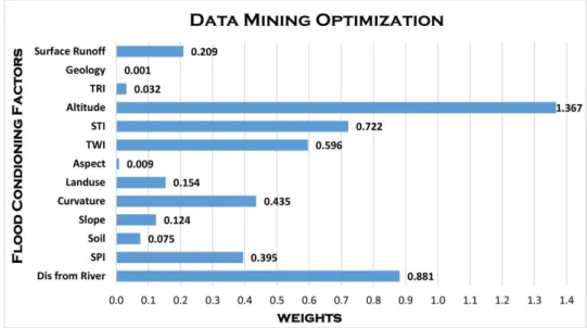
modelling. As mentioned earlier, RBF kernel was used to generate aflood probability map in GIS environment. The probability index ranged from 0 to 1.Figure 8shows ensemble FR-SVM optimi-zation result andFigure 9demonstrates theflood probability map generated from the ensemble FR-SVM model. The highest probability offlood occurrence is located in regions with the lowest eleva-tion and direceleva-tion of the basin outlet.
Based on the result of ensemble SVM and FR modelling which as shown inFigure 8, geology, aspect, TRI and soil factors are achieved the lowest rank, respectively, and consider insignificant withflood probability in our study area. However, Altitude, Distance from River, STI and TWI are the most significant parameters which are related toflood occurrence, respectively. The correlation coefficient of this model was estimated as 0.7413 and mean absolute error was 0.2453.
Therefore, each class of conditioning factors along with each conditioning factor has been opti-mized by ensemble FR and SVM model. Then all weighted layers were overlaid to generate theflood probability map.
5.2. Flood risk mapping
In this study, aflood risk map was mainly derived from the combination of the hazard and vulnera-bility maps as discussed earlier. During thefirst phase of this research, the ensemble of the FR and SVM model was used to investigate flood probability across the catchment. During the second phase, after the probability map was obtained, rainfall andflood inundation depth were selected as the main triggering factor to combine with the probability of acquiring the hazard map as illustrated inEquation (13). Afinal hazard map ranging from 0 to 1 was obtained as a result of this combina-tion. The highest hazard level occurs in the southern part of the study area, where the elevation toward the basin outlet is decreased.Figure 10shows the classified hazard map of the study area.
In a next phase, after thefinal hazard map was prepared, the vulnerability map was evaluated as a second initial component of the risk map. The vulnerability map was derived by relying on the data collected from GIS maps with information on detailed land-use types. As mentioned earlier, the land-use map was prepared using very high resolution satellite images from WorldView-3. The overall accuracy of classification was at 84.07%, which could be considered accurate as previously illustrated inTable 3. The value of a criterion was assigned to each element at risk based on their
importance in the study area. The majority of the catchment area is also covered by built-up land, where most of the residential areas and commercial centres are located. After the highway, vulnera-bility criteria value (5) was assigned to the built-up land. The second highest value of vulnerability (4) in this area was allocated to the highway because it is located at a lower elevation compared with the built-up land. In case offlood occurrence across the highway, loss of human lives and damage to properties will occur across the highway. Furthermore, the rescue operation of emergency workers, such asfirefighters, police officers, and medical personnel, in the built-up land will be interrupted and delayed. Therefore, on the basis of expert opinion, the highway was determined as the second most vulnerable element at risk in the study area. The lower vulnerability value based on expert opinion was assigned to the road (3) and recreation area (2). However, the lowest vulnerability value (1) was allocated to areas covered by forest because they are densely vegetated, which reduces the speed of runoff.
Thefinal stage of this research aims to determineflood risk in the study area based on the quanti-tative approach. Therefore, theflood hazard and vulnerability maps were combined to produce a direct specific risk map usingEq. 12, and aflood risk map ranging from 0 to 1 was achieved, then thefinal risk map was split into classified risk areas to improve visual interpretation. Hence, the
flood risk levels were clearly recognized. When classifying theflood risk map into categorical classes, a quantile method was applied. This classifier is commonly recommended for this objective because it uses mean values to create class breaks. Five risk levels, namely, no risk, low, moderate, high, and Figure 9.Flood probability map for Damansara river catchment.
very high, were distinguished using this approach (Figure 11). The percentages of each risk level in the study area are also presented inTable 4. No risk and low-risk areas cover 42.8% of the entire catchment. Moderateflood risk (30.2% of the catchment) is also depicted in regions close to the high- and very high risk zones in the study area. The high areas cover 22.6% and very high risk areas cover only 4.2% of the catchment.
5.3. Validation andfield verification
The efficiency of theflood hazard map using the ensemble model was evaluated via receiver-operat-ing characteristic (ROC) curve. The success rate and prediction rate curves were evaluated. The suc-cess rate and prediction rate curves were produced using theflood training data set (70%) and the
flood validation data set (30%), respectively. The results are 89.7% and 78.9% for the success and prediction rates, respectively (Figure 12).
Furthermore, multiplefield visits were conducted to verify the derived results (Figure 13). The
flood location and condition was recorded during the fluvialflood events on 12 and 27 October 2014, 13 and 29 January 2015, and 18 February 2015. Expectedly, all the recorded inventory points fell within the high-risk and very high risk zones, where the probability offlood was very high. This process presents a good verification of the reliability of the applied model in the study area.
6. Conclusion
Flood occurrence is a serious and disastrous event that can happen practically anywhere. Therefore, controlling the effects offlood is crucial, and can be performed viaflood hazard and risk mapping. Flood-prone areas must be identified to anticipate and analyse the spatial distribution of appropriate
flood management in the future. The research background indicates that various methods and tech-niques have been applied to identifyflood-susceptible areas. In the current research, the GIS-based ensemble method of FR and SVM was used in theflood hazard mapping of the study area along Figure 11.Flood risk levels of the study area.
Table 4.The area percentage of risk map for Damansara river catchment.
Code Class Area (m2) Area (km2) Percentage
1 Very low 14900472.19 14.90 12.75 2 Low 35307217.61 35.31 30.21 3 Moderate 35329035.80 35.33 30.23 4 High 26440455.04 26.44 22.63 5 Very high 4880703.38 4.88 4.18 Total 116857884.03 116.86 100%
NKVE, and the location of the study area at Sungai Damansara is highly susceptible toflood occur-rence. The Sungai Damansara catchment was used in the case study, and 13 indices were selected to construct the evaluation system. In the case of topographical data, DEM was built from IFSAR images with a pixel size of 5 m£5 m. Furthermore, LULC mapping, which was one of the effective parameters of flooding, and vulnerability assessment were extracted from WorldView-3 satellite imagery with 0.3 m spatial resolution. Each conditioning factor was optimized using the FR approach and entered as input for SVM modelling. The correlation between eachflood-related fac-tor andflood location showed that areas with a low elevation, mild slope, andflat curvature exhibit the highest probability offlood occurrence. The accuracy of theflood probability indices obtained from this ensemble method was validated using AUC. The estimated success rate and prediction rate of the applied method was at 89.7% and 78.9%, respectively. The most effective parameters that would triggerflood occurrence in the study area were rainfall andflood inundation depth. Thus, it was used as the triggering factor forflood hazard estimation. Rainfall data were derived from nine rainfall stations in and around the study area within the last 5 years andflood inundation depth was generated using hydraulic 2D HRS model. Furthermore, weights ranging from 1 to 5 were assigned to the most vulnerable elements, which were selected based on precise land-use information. As the main objective of this research, the risk level map wasfinally produced based on hazard and vulnera-bility indices. The reliavulnera-bility of the results obtained from this study was also verified in thefield. Consequently, the ensemble method of FR and SVM can be efficiently used inflood hazard studies because of its simple structure and robust performance. Furthermore, the FR model is an excellent approach for ranking different classes of conditioning parameters. Therefore, each index map derived from this study can be helpful to planners and decision makers forflood management and planning in the study area.
Disclosure statement
No potential conflict of interest was reported by the authors.
ORCID
Biswajeet Pradhan http://orcid.org/0000-0001-9863-2054
References
Akgun A, Dag S, Bulut F.2007. Landslide susceptibility mapping for a landslide-prone area (Findikli, NE of Turkey)
by likelihood-frequency ratio and weighted linear combination models. Environ Geol. 54:1127–1143. doi:10.1007/
s00254-007-0882-8.
Althuwaynee OF, Pradhan B, Lee S.2012. Application of an evidential belief function model in landslide susceptibility
mapping. Comput Geosci. 44:120–135. doi:10.1016/j.cageo.2012.03.003.
Apel H, Aronica GT, Kreibich H, Thieken AH.2008. Flood risk analyses–how detailed do we need to be? Nat
Haz-ards. 49:79–98. doi:10.1007/s11069-008-9277-8.
Ayalew L, Yamagishi H.2005. The application of GIS-based logistic regression for landslide susceptibility mapping in
the Kakuda-Yahiko Mountains, Central Japan. Geomorphology. 65:15–31. doi:10.1016/j.geomorph.2004.06.010.
Botzen WJW, Aerts JCJH, van den Bergh JCJM.2012. Individual preferences for reducingflood risk to near zero
through elevation. Mitig Adapt Strateg Glob Change. 2:229–244. doi:10.1007/s11027-012-9359-5.
Casulli, V.2009. A highresolution wetting and drying algorithm for freesurface hydrodynamics. Int J Numerical
Methods Fluids. 60:391–408.
Chau KW, Wu CL, Li YS.2005. Comparison of severalflood forecasting models in Yangtze River. J Hydrol Eng. 10:
485–491. doi:10.1061/(asce)1084-0699(2005)10:6(485).
Choi J, Oh HJ, Won JS, Lee S.2009. Validation of an artificial neural network model for landslide susceptibility
map-ping. Environ Earth Sci. 60:473–483. doi:10.1007/s12665-009-0188-0.
Gokceoglu C, Sonmez H, Nefeslioglu HA, Duman TY, Can T.2005. The 17 March 2005 Kuzulu landslide (Sivas,
Tur-key) and landslide-susceptibility map of its near vicinity. Eng Geol. 81:65–83. doi:10.1016/j.enggeo.2005.07.011.
Horritt MS.2006. A methodology for the validation of uncertainflood inundation models. J Hydrol. 326:153–165.
doi:10.1016/j.jhydrol.2005.10.027.
Rizeei HM, Saharkhiz MA, Pradhan B, Ahmad N.2016. Soil erosion prediction based on land cover dynamics at the
Semenyih watershed in Malaysia using LTM and USLE models. Geocarto Int. 31:1158–1177. doi: 10.1080/
10106049.2015.1120354.
Huong HTL, Pathirana A.2013. Urbanization and climate change impacts on future urbanflooding in Can Tho city,
Vietnam. Hydrol Earth Syst Sci. 17:379–394. doi:10.5194/hess-17-379-2013.
Intergovernmental Panel on Climate Change,2014. Summary for policy makers. In: Field CB, Barros VR, Dokken DJ,
Mach KJ, Mastrandrea MD, Bilir MCTE, Ebi KL, Estrada YO, Genova RC, Girma B, Kissel ES, Levy AN, Mac-Cracken S, Mastrandrea a.L.L.W.e.P.R. editors. Climate change 2014: impact, adaptation, and vulnerability. Part a:
global and sectoral aspects. Contribution of working group II to thefifth assessment report of the
intergovernmen-tal panel on climate change. Cambridge (UK): Cambridge University Press; p. 1–32.
Jebur MN, Pradhan B, Tehrany MS.2014a. Optimization of landslide conditioning factors using very high-resolution
airborne laser scanning (LiDAR) data at catchment scale. Remote Sens Environ. 152:150–165. doi:10.1016/j.
rse.2014.05.013.
Kar AK, Lohani AK, Goel NK, Roy GP.2015. Rain gauge network design forflood forecasting using multi-criteria
decision analysis and clustering techniques in lower Mahanadi river basin, India. J Hydrol: Reg Stud. 4:313–332.
doi:10.1016/j.ejrh.2015.07.003.
Kia MB, Pirasteh S, Pradhan B, Mahmud AR, Sulaiman WNA, Moradi A.2011. An artificial neural network model for
flood simulation using GIS: Johor River Basin, Malaysia. Environ Earth Sci. 67:251–264.
doi:10.1007/s12665-011-1504-z.
Lecca G, Petitdidier M, Hluchy L, Ivanovic M, Kussul N, Ray N, Thieron V.2011. Grid computing technology for
hydrological applications. J Hydrol. 403:186–199.
Lee MJ, Kang J, Jeon S.2012. Application of frequency ratio model and validation for predictiveflooded area
suscepti-bility mapping using GIS. 2012 IEEE International Geoscience and Remote Sensing Symposium. doi:10.1109/ igarss.2012.6351414.
Manandhar B.2010. Flood plain analysis and risk assessment of Lothar Khola, MSc Thesis, Phokara: Tribhuvan
Uni-versity; p. 64.
MarjanovicM, Kovacevic M, Bajat B, Vozenılek V.2011. Landslide susceptibility assessment using SVM machine
learning algorithm. Eng Geol. 123:225–234.
Merz B, Kreibich H, Lall U.2013. Multi-variateflood damage assessment: a tree-based data-mining approach. Nat
Hazard Earth Sys. 13:53–64. doi:10.5194/nhess-13-53-2013.
Meyer V, Scheuer S, Haase D.2008. A multicriteria approach forflood risk mapping exemplified at the Mulde river,
Germany. Nat Hazards. 48:17–39. doi:10.1007/s11069-008-9244-4.
Moore ID, Wilson JP.1992. Length-slope factors for the revised universal soil loss equation: simplified method of
esti-mation. J Soil Water Conserv. 47:423–428.
M€uller A, Reiter J, Weiland U.2011. Assessment of urban vulnerability towardsfloods using an indicator-based
approach–a case study for Santiago de Chile. Nat Hazards Earth Syst Sci. 11:2107–2123.
Neshat A, Pradhan B.2015. An integrated DRASTIC model using frequency ratio and two new hybrid methods for
groundwater vulnerability assessment. Nat Hazards. 76:543–563.
Pradhan B.2009. Groundwater potential zonation for basaltic watersheds using satellite remote sensing data and GIS
techniques. Open Geosci. 1:120–129. doi:10.2478/v10085-009-0008-5.
Pradhan B.2010. Flood susceptible mapping and risk area delineation using logistic regression, GIS and remote
sens-ing. J Spatial Hydrol. 9:1–18.
Pradhan B, Hagemann U, Tehrany, MS, Prechtel N.2014. An easy to use ArcMap based texture analysis program for
extraction of flooded areas from TerraSAR-X satellite image. Comput Geosci. 63:34–43. doi:10.1016/j.
cageo.2013.10.011.
Samui P.2008. Support vector machine applied to settlement of shallow foundations on cohesionless soils. Comput
Geotech. 35:419–427. doi:10.1016/j.compgeo.2007.06.014.
Song S, Zhan Z, Long Z, Zhang J, Yao L.2011. Comparative study of SVM methods combined with voxel selection for
object category classification on fMRI Data. PLoS ONE. 6:e17191. doi:10.1371/journal.pone.0017191.
Stefanidis S, Stathis D.2013. Assessment offlood hazard based on natural and anthropogenic factors using analytic
hierarchy process (AHP). Nat Hazards. 68:569–585. doi:10.1007/s11069-013-0639-5.
Tehrany MS, Pradhan B, Jebur MN.2014. Flood susceptibility mapping using a novel ensemble weights-of-evidence
and support vector machine models in GIS. J Hydrol. 512:332–343. doi:10.1016/j.jhydrol.2014.03.008.
Tehrany MS, Pradhan B, Jebur MN.2013. Spatial prediction offlood susceptible areas using rule based decision tree
(DT) and a novel ensemble bivariate and multivariate statistical models in GIS. J Hydrol. 504:69–79. doi:10.1016/j.
jhydrol.2013.09.034.
Tien Bui, D., Pradhan, B., Lofman, O., Revhaug, I.,2012a. Landslide susceptibility assessment in Vietnam using
sup-port vector machines, decision tree, and Na€ıve Bayes Models. Math Probl Eng. 2012:1–26. doi:10.1155/2012/
974638.
Tingsanchali T, Karim F.2010. Flood-hazard assessment and risk-based zoning of a tropicalflood plain: case study of
the Yom River, Thailand. Hydrol Sci J. 55:145–161. doi:10.1080/02626660903545987.
Tunusluoglu MC, Gokceoglu C, Nefeslioglu HA, Sonmez H.2007. Extraction of potential debris source areas by
logis-tic regression technique: a case study from Barla, Besparmak and Kapi mountains (NW Taurids, Turkey). Environ
Geol. 54:9–22. doi:10.1007/s00254-007-0788-5.
Vojinovic Z, Abbott MB.2012. Flood risk and social justice: from quantitative to qualitativeflood risk assessment and
mitigation. Water Intell. Online 11. London (UK): IWA Publishing. ISBN: 9781780400822. Horritt, 2006.
Yalcin A, Reis S, Aydinoglu AC, Yomralioglu T.2011. A GIS-based comparative study of frequency ratio, analytical
hierarchy process, bivariate statistics and logistics regression methods for landslide susceptibility mapping in
Trab-zon, NE Turkey. CATENA. 85:274–287. doi:10.1016/j.catena.2011.01.014.
Yao X, Tham L, Dai F.2008. Landslide susceptibility mapping based on support vector machine: a case study on
natu-ral slopes of Hong Kong, China. Geomorphology. 101:572–582.
Zhou J, Deng W, Zou Q, Xiao J, Zhang Y, Hua W.2013. Flood disaster evaluation model based on kernel dual