Kiran Lakhotia
Department of Computer Science King’s College London
Submitted in partial fulfilment of the requirements for the degree of Doctor of Philosophy at King’s College London
This thesis is concerned with the problem of automatic test data genera-tion for structural testing criteria, in particular the branch coverage ade-quacy criterion, using search–based techniques. The primary objective of this thesis is to advance the current state–of–the–art in automated search– based structural testing. Despite the large body of work within the field of search–based testing, the accompanying literature remains without con-vincing solutions for several important problems, including: support for pointers, dynamic data structures, and loop–assigned flag variables. Fur-thermore, relatively little work has been done to extend search–based testing to multi–objective problem formulations.
One of the obstacles for the wider uptake of search–based testing has been the lack of publicly available tools, which may have contributed to the lack of empirical studies carried out on real–world systems. This thesis presents AUSTIN, a prototype structural test data generation tool for the C lan-guage. The tool is built on top of the CIL framework and combines a hill climber with a custom constraint solver for pointer type inputs. AUSTIN has been applied to five large open source applications, as well as eight non– trivial, machine generated C functions drawn from three real–world embed-ded software modules from the automotive sector. Furthermore, AUSTIN has been compared to a state–of–the–art Evolutionary Testing Framework and a dynamic symbolic execution tool, CUTE. In all cases AUSTIN was shown to be competitive, both in terms of branch coverage and efficiency. To address the problem of loop–assigned flags, this thesis presents a testa-bility transformation along with a tool that transforms programs with loop– assigned flags into flag–free equivalents, so that existing search–based test data generation approaches can successfully be applied.
I would like to thank my supervisor Professor Mark Harman for provid-ing this opportunity, and for his endless support and advice throughout this PhD. I would also like to thank my second supervisor, Dr Kathleen Steinh¨ofel, for her support and comments, especially during the early stages of this PhD.
In addition, I am very grateful to Berner & Mattner GmbH, and in particu-lar Dr Joachim Wegener, for providing me with the opportunity to evaluate AUSTIN on real–world code. Thanks also to Laurence Tratt for his helpful comments on the thesis and Arthur Baars for taking the time to explain the Evolutionary Testing Framework. I would further like to thank all the co–authors of the papers I have published, partly as a result of this work, for all their hard work and all the anonymous referees for their comments and feedback, as these have been extremely beneficial. Thanks also to Dr Phil McMinn for making the IGUANA testing framework available to me and to all my colleagues in CREST for their support and discussions. The achievements of this thesis would not have been possible without the support of my parents who provided me with the opportunity to pursue my interest in computer science, and my partner, Helen Hudson, who I would like to thank for her love, support, and patience during the three years of this project.
I herewith declare that I have produced this thesis without the prohibited assistance of third parties and without making use of aids other than those specified; notions taken over directly or indirectly from other sources have been identified as such.
The thesis work was conducted from September 2006 to September 2009 under the supervision of Professor Mark Harman at King’s College London. Some of this work has been accepted to appear in the refereed literature:
1. D. Binkley, M. Harman, K. Lakhotia, FlagRemover: A Testability Transformation For Loop Assigned Flags, Transactions on Software Engineering and Methodology (TOSEM), To appear.
2. K. Lakhotia, P. McMinn, M. Harman, Automated Test Data Genera-tion for Coverage: Haven’t We Solved This Problem Yet?,4th Testing Academia and Industry Conference - Practice and Research Techniques (TAIC PART 09), Windsor, UK, 4th–6th September 2009, To appear. 3. M. Harman, K. Lakhotia, P. McMinn, A Multi–Objective Approach to Search-Based Test Data Generation,Proceedings of the Genetic and Evolutionary Computation Conference (GECCO 2007), London, UK, July 7–11, 2007, pp. 1098-1105, ACM Press.
In addition to the above, during the programme of study, I have published the following papers, the work of which does not feature in this thesis:
1. K. Lakhotia, M. Harman, P. McMinn, Handling Dynamic Data Struc-tures in Search Based Testing, Proceedings of the Genetic and Evolu-tionary Computation Conference (GECCO 2008), Atlanta, USA, July 12–16, 2008, pp. 1759–1766, ACM Press.1
ation,Proceedings of the ACM SIGSOFT Symposium on the Founda-tions of Software Engineering (FSE 2007), Cavtat, Croatia, September 3–7, 2007, pp. 155–164, ACM Press.
List of Figures ix
List of Tables xvii
1 Introduction 1
1.1 The Problem Of The Thesis: Practical Challenges For Automated Test
Data Generation . . . 3
1.2 Aims and Objectives . . . 4
1.3 Contributions Of The Thesis . . . 5
1.4 Overview Of The Structure Of The Thesis . . . 6
1.5 Definitions . . . 7
1.5.1 Input Domain . . . 7
1.5.2 Control and Data Dependence . . . 8
2 Literature Review 13 2.1 Search–Based Testing . . . 13
2.1.1 Genetic Algorithms . . . 17
2.1.2 Hill Climb . . . 20
2.1.3 Fitness Functions . . . 21
2.2 Static Analysis Based Testing . . . 24
2.2.1 Symbolic Execution . . . 25
2.2.2 Dynamic Symbolic Execution . . . 27
3 Augmented Search–Based Testing 35 3.1 Introduction . . . 35
3.2.1 Floating Point Variables . . . 37
3.2.2 Example . . . 40
3.2.3 Code Preparation . . . 41
3.2.4 Symbolic Rewriting . . . 44
3.2.5 Pointer Inputs . . . 49
3.2.5.1 Limitations of Pointer Rules . . . 54
3.2.6 The Algorithm . . . 58
3.2.7 Input Initialization . . . 65
3.2.7.1 Limitations of Input Types . . . 66
3.2.8 Usage . . . 69
3.3 Evolutionary Testing Framework . . . 70
3.4 Empirical Study . . . 71
3.4.1 Experimental Setup . . . 75
3.4.2 Evaluation . . . 78
3.4.3 Threats to Validity . . . 84
3.5 Conclusion . . . 86
4 An Empirical Investigation Comparing AUSTIN and CUTE 87 4.1 Introduction . . . 87
4.2 CUTE . . . 89
4.3 Motivation and Research Questions . . . 89
4.4 Empirical Study . . . 91
4.4.1 Test Subjects . . . 91
4.4.2 Experimental Setup . . . 92
4.4.3 Answers to Research Questions . . . 93
4.4.3.1 CUTE–specific issues . . . 101
4.4.3.2 AUSTIN–specific issues . . . 103
4.5 Threats to Validity . . . 105
4.6 Discussion: Open Problems in Automated Test Data Generation . . . . 106
4.7 Related Work . . . 107
5 Testability Transformation 109
5.1 Introduction . . . 109
5.2 Background . . . 111
5.2.1 The Flag Problem . . . 111
5.2.2 Testability Transformation . . . 112
5.3 The Flag Replacement Algorithm . . . 112
5.4 Implementation . . . 118
5.4.1 Definition of Loop–Assigned Flag . . . 118
5.4.2 Flag Removal . . . 120
5.4.3 Runtime . . . 121
5.4.4 Limitations . . . 121
5.5 Empirical Algorithm Evaluation . . . 123
5.5.1 Synthetic Benchmarks . . . 123
5.5.2 Open Source and Daimler Programs . . . 128
5.6 Relevant Literature For the Loop–Assigned Flag Problem . . . 137
5.7 Conclusion . . . 139
6 Multi–Objective Test Data Generation 141 6.1 Introduction . . . 141
6.2 Background . . . 143
6.3 Implementation . . . 145
6.3.1 Pareto Genetic Algorithm Implementation . . . 146
6.3.2 Weighted Genetic Algorithm Implementation . . . 147
6.4 Experimental Setup . . . 148
6.5 Case Study Results . . . 148
6.6 Discussion . . . 151
6.7 Conclusion . . . 156
7 Conclusions and Future Work 157 7.1 Summary of Achievements . . . 157
7.2 Summary of Future Work . . . 160
A Abbreviations and Acronyms 165
1.1 Code template in the left column is used to illustrate search–based test data generation. In the right column is the CFG of the code in the left column. The CFG is annotated with the approach levelfor node 4. . . . 9 1.2 A code example with the corresponding CFG on the right illustrating
how data flow information is not captured explicitly in a CFG. The true branch of node 4 is data dependent on node 3, but not control dependent on any other node except the start node. . . 11 2.1 Example used to demonstrate Korel’s goal oriented (Kor92) test data
generation approach. . . 16 2.2 A typical evolutionary algorithm for testing. . . 18 2.3 Example illustrating how the crossover operator in a GA combines parts
of two candidate solutions, Candidate String 1 and Candidate String 2, to form an offspring representing the desired string. . . 19 2.4 Example used to illustrate how machine semantics differ from
mathemat-ical principles over reals and rational numbers. Arithmetic suggests that the path<1,2,3,4,5> is infeasible, when in practice there exist values for x that satisfy this path. . . 27 2.5 Example for demonstrating dynamic symbolic execution. The branch
predicate is non–linear. . . 28 2.6 Example for demonstrating pointer handling in CUTE. . . 30 2.7 Code example used to illustrate how the EVACON framework (IX07)
is able to optimize both, the method call sequences required to test the functionm, as well as the method parameters to achieve coverage of m. 33
3.1 Example C code used for demonstrating how AUSTIN combines custom constraint solving rules for pointer inputs with an AVM for other inputs to a function under test. The goal is to find an input which satisfies the condition at node 2. . . 38 3.2 Pseudo code illustrating the method for checking if the search is stuck at
a local optimum. Part of this method also includes the steps for varying the accuracy of floating point variables as described in Section 3.2.1. . . 39 3.3 Example for demonstrating how AUSTIN optimizes floating point type
inputs. Previous work (MH06; LMH09) commonly fixed the accuracy for floating point variables in the AVM to 1 or 2 decimal places. Such a strategy suffices to generate inputs to satisfy the branch predicate in the left column, but is unlikely to succeed for the branch predicate in the right column. AUSTIN is able to automatically satisfy the branch predicates in both the left and right columns. . . 40 3.4 Two examples illustrating how CIL transforms compound predicates into
single predicate equivalents. The transformation works for both, predi-cates in conditional statements (see (a)) and in–line predipredi-cates (see (b)). 43 3.5 Ocaml type declarations in AUSTIN used to denote symbolic lvalues and
symbolic terms. A symbolic lvalue is used to represent an input variable to the function under test, while symbolic terms provide a wrapper for CIL expressions. Symbolic terms only consist of operations involving constants or input variables to the function under test. . . 45 3.6 Code snippet illustrating the Ocaml class for rewriting CIL expressions
in terms of input variables. The class extends CIL’s default visitor, which traverses a CIL tree without modifying anything. The methodvexpr is invoked on each occuring (CIL) expression. The subtrees are the sub– expressions, the types (for a cast or sizeof expression) or the variable use. . . 47
3.7 The example in the top half demonstrates how symbols are updated in a symbolic store using the visitor class from Figure 3.6. The bottom row shows how AUSTIN approximates symbolic expressions with the help of concrete runtime values instead of performing symbolic pointer arithmetic. The expression((struct item **)(tmp1 + 8))is replaced by the expression denoting the address of one->next, i.e. &one->next, instead of rewriting the expression as((struct item **)(((unsigned long)one) + 8))using the visitor class from Figure 3.6. . . 48 3.8 Code snippet used as a running example to explain AUSTIN’s pointer
solving rules. . . 51 3.9 An example illustrating how AUSTIN builds up an equivalence graph of
symbolic terms over successive executions. The graph is used to instan-tiate the concrete pointer type inputs to the function under test. The example shows the evolution of the graph when node 5 has been selected as target. . . 53 3.10 Pseudo code illustrating the algorithm for constructing an equivalence
graph. The graph forms the basis for deriving values assigned to pointer inputs of a function under test. . . 55 3.11 Pseudo code illustrating the algorithm for assigning concrete values to
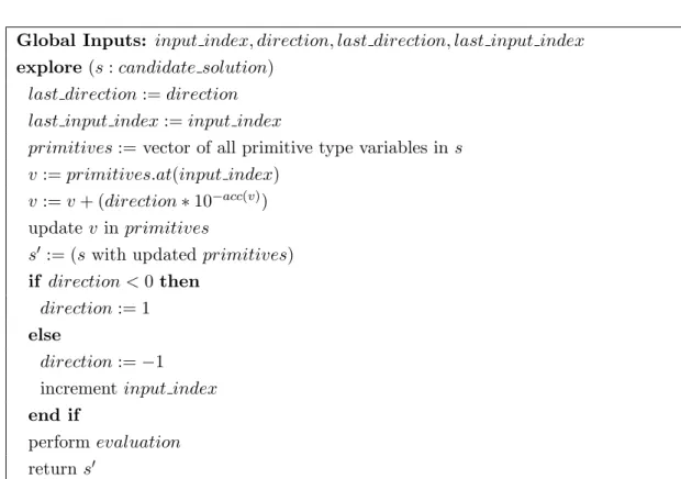
pointers. The manner in which new or existing memory locations are assigned to a function’s pointer inputs depends on the structure of the equivalence graph. . . 56 3.12 Pseudo code showing the top level search algorithm implemented in
AUSTIN. It extends a hill climber to include constraint solving rules for pointer inputs to a function under test. The steps for handling nu-merical type inputs to a function under test are based on the alternating variable method introduced by Korel (Kor90). . . 59 3.13 Pseudo code illustrating the algorithm for performing exploratory moves
which are part of the alternating variable method. . . 61 3.14 Pseudo code illustrating the algorithm for performing pattern moves in
the alternating variable method. Pattern moves are designed to speed up the search by accelerating towards an optimum. . . 62
3.15 Pseudo code illustrating the algorithm for optimisingn–valued enumer-ation type variables, variables that can only take on n discrete values. Whenever an enumeration type variable is to be optimized, the algo-rithm iterates over all nvalues (in the order they have been declared in the source code). . . 63 3.16 Pseudo code illustrating the method for checking if AUSTIN should use
its custom constraint solving rules for pointers, or the alternating vari-able method to satisfy the constraint in a branching node. . . 64 3.17 Pseudo code illustrating the reset operation performed by AUSTIN at
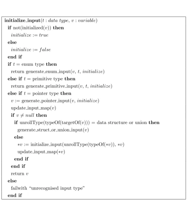
every random restart. . . 65 3.18 Pseudo code illustrating the entry point for initializing a candidate
so-lution (i.e. the inputs to the function under test) with concrete values. . 66 3.19 Pseudo code illustrating the method assigning concrete values to an input
variable of the function under test. . . 67 3.20 This group of methods shows the pseudo code for assigning values to
inputs of the function under test, based on their type declaration. . . 68 3.21 Pseudo code illustrating how AUSTIN instantiates its map of concrete
values mC and address map mA at the start of every execution of the
function under test. The maps are also updated during the dynamic execution of the function under test. . . 69 3.22 Example showing how the ETF initializes pointers to primitive types.
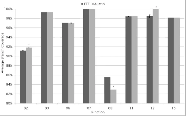
The chromosome only shows the parts which relate to the two pointer inputspandq. The first component of each pair denotes an index (of a variable in a pool) while the second component denotes a value. . . 72 3.23 Average branch coverage of the ETF versus AUSTIN (N ≥ 30). The
y−axis shows the coverage achieved by each tool in percent, for each of the functions shown on thex−axis. The error bars show the standard error of the mean. Bars with a∗ on top denote a statistically significant difference in the mean coverage (p≤0.05). . . 79
3.24 Average branch coverage of random search versus AUSTIN (N ≥ 29). The y−axis shows the coverage achieved by each tool in percent, for each of the functions shown on the x−axis. The error bars show the standard error of the mean. Bars with a ∗ on top denote a statistically significant difference in the mean coverage (p≤0.05). . . 81 3.25 Average number of fitness evaluations (normalized) for ETF versus AUSTIN
(N ≥30). They−axisshows the normalized average number of fitness evaluations for each tool relative to the ETF (shown as 100%) for each of the functions shown on thex−axis. The error bars show the standard error of the mean. Bars with a∗on top denote a statistically significant difference in the mean number of fitness evaluations (p≤0.05). . . 82 3.26 Average number of fitness evaluations (normalized) for random versus
AUSTIN (N ≥29). They−axisshows the normalized average number of fitness evaluations for each tool relative to the random search (shown as 100%) for each of the functions shown on thex−axis. The error bars show the standard error of the mean. Bars with a∗on top denote a sta-tistically significant difference in the mean number of fitness evaluations (p≤0.05). . . 84 4.1 Branch coverage for the test subjects with CUTE and AUSTIN. CUTE
explicitly explores functions called by the function under test, whereas AUSTIN does not. Therefore the graph 4.1(a) counts only branches cov-ered in each function tested individually. Graph 4.1(b) counts branches covered in the function under test and branches covered in any func-tions called. Graph 4.1(c) is graph 4.1(b) but with certain funcfunc-tions that CUTE cannot handle excluded. . . 94 4.2 An example used to illustrate how a random restart in AUSTIN can
affect the runtime of a function under test, and thus the test data gen-eration process. Very large values of upbmay have a significant impact on the wall clock time of the test data generation process. . . 98
5.1 This figure uses three fitness landscapes to illustrate the effect flag vari-ables have on a fitness landscape, and the resulting ‘needle in a haystack’ problem. The figure has been taken from the paper by Binkley et al.(BHLar). . . 110 5.2 An example program before and after applying the coarse and fine–
grain transformations. The figures also shows part of the function for computing local fitness. . . 114 5.3 The transformation algorithm. Suppose thatflag is assignedtrue
out-side the loop and that this is to be maintained. . . 116 5.4 Results over ten runs of the evolutionary search for each of the two
transformation approaches. The graphs have been taken from the paper by Baresel et al. (BBHK04). . . 125 5.5 Results over ten runs of the evolutionary search for the fine–grained
transformation approach close–up. The graph has been taken from the paper by Baresel et al. (BBHK04). . . 126 5.6 Results over ten runs of the alternating variable method for the ‘no
transformation’ and fine–grained transformation approaches. . . 127 5.7 Chart of data from second empirical study. . . 136 6.1 Results of the branch coverage and memory allocation achieved by three
different algorithms: a random search, a Pareto GA and, weighted GA. 152 6.2 Final Pareto fronts produced for targets 1T and 1F. The upper point on
the y–axis represents the ‘ideal’ solution for target 1F. As can be seen, once the branch has been reached, a single solution will dominate all oth-ers because it is the only branch allocating memory. When attempting to cover target 1T on the other hand, the Pareto optimal set potentially consists of an infinite number of solutions. The graph combines five runs which reveal little variance between the frontlines produced. Interest-ingly, the ‘ideal’ point for target 1F corresponds to the maximum value contained within the Pareto optimal set for target 1T with respect to memory allocation. . . 154
6.3 The table at the bottom presents the Pareto optimal sets for each ‘sub– goal’ of the example function above used in Case Study 2. It combines the results collected over five runs and illustrates that it is often not possible to generate a Pareto frontline when considering branch coverage and memory allocation as a MOP. Although the amount of dynamic memory allocated depends on the input parameters, it is constant for all branches. As a result one solution will dominate all others with respect to a particular target. . . 155 7.1 Code example to illustrate ideas for future work. . . 162
2.1 Branch functions for relational predicates introduced by Korel (Kor90). 14 2.2 Branch distance measure introduced by Tracey (Tra00) for relational
predicates. The valueK is a failure constant which is always added if a term is false. . . 23 2.3 Objective functions introduced by Tracey (Tra00) for conditionals
con-taining logical connectives. z is one of the objective functions from Ta-ble 2.2. . . 23 2.4 Dynamic data structure creation according to individual constraints
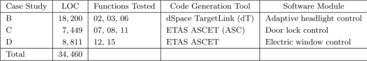
en-countered along the path condition for CUTE. . . 31 3.1 Case studies. LOC refers to the total preprocessed lines of C source
code contained within the case studies. The LOC have been calculated using the CCCC tool (Lit01) in its default setting. Table 3.2 shows the individual per–function LOC metric. . . 72 3.2 Test subjects. The LOC have been calculated using the CCCC tool (Lit01)
in its default setting. The number of input variables counts the number of independent input variables to the function,i.e. the member variables of data structures are all counted individually. . . 74 3.3 Summary of functions with a statistically significant difference in the
branch coverage achieved by AUSTIN and the ETF. The columns Std-Dev indicate the standard deviation from the mean for ETF and AUSTIN. The t value column shows the degrees of freedom (value in brackets) and the result of the t–test. Ap value of less than 0.05 means there is a sta-tistically significant difference in the mean coverage between ETF and AUSTIN. . . 78
3.4 Summary of functions with statistically significant differences in the number of fitness evaluations used. The columns StdDev indicate the standard deviation from the mean for ETF and AUSTIN. The t value column shows the degrees of freedom (value in brackets) and the result of the t–test. A p value of less than 0.05 means there is a statistically significant difference in the mean number of fitness evaluations between ETF and AUSTIN. . . 83 4.1 Details of the test subjects used in the empirical study. In the ‘Functions’
column, ‘Non–trivial’ refers to functions that contain branching state-ments. ‘Top–level’ is the number of non–trivial, public functions that a test driver was written for, whilst ‘tested’ is the number of functions that were testable by the tools (i.e. top–level functions and those that could be reached interprocedurally). In the ‘Branches’ column, ‘tested’ is the number of branches contained within the tested functions. . . 90 4.2 Test subjects used for comparing wall clock time and interprocedural
branch coverage. . . 95 4.3 Interprocedural branch coverage for the sample branches from Table 4.2
and the wall clock time taken to achieve the respective levels of coverage. 96 4.4 Errors encountered for test data generation for the sample of branches
listed in Table 4.3. . . 99 5.1 Runtime of the transformation (in seconds) for the test subjects as
re-ported by the time utility. The measurements are averaged over five runs. The column real refers to the wall clock time, user refers to the time used by the tool itself and any library subroutines called, whilesys indicates the time used by system calls invoked by the tool. . . 122 5.2 Test subjects for the evaluation of the transformation algorithm. . . 129 5.3 Branch coverage results from empirical study of functions extracted from
open source software. . . 134 5.4 Fitness function evaluations from empirical study of functions extracted
6.1 The table shows the branches covered by the weighted GA and not the Pareto GA, or vice versa. The ‘distance’ measure illustrates how close the best solution came to traversing the target branch. It combines the normalized branch distance and the approach level. A distance of 0 indicates a branch has been covered. These results were obtained during Case Study 1. . . 156
Introduction
In recent years there has been a particular rise in the growth of work on Search–Based Software Testing (SBST) and, specifically, on techniques for generating test data that meet structural coverage criteria such as branch– or modified condition / decision cov-erage. The field of search–based software engineering reformulates software engineering problems as optimization problems and uses meta–heuristic algorithms to solve them. Meta–heuristic algorithms combine various heuristic methods in order to find solutions to computationally hard problems where no problem specific heuristic exists. SBST was the first software engineering problem to be attacked using optimization (MS76) and it remains the most active area of research in the search–based software engineering community.
Software testing can be viewed as a sequence of three fundamental steps:
1. The design of test cases that are effective at revealing faults, or which are at least adequate according to some test adequacy criterion.
2. The execution of these test cases.
3. The determination of whether the output produced is correct.
Sadly, in current testing practice, often the only fully automated aspect of this ac-tivity is test case execution. The problem of determining whether the output produced by the program under test is correct cannot be automated without an oracle, which is seldom available. Fortunately, the problem of generating test data to achieve widely
used notions of test adequacy is an inherently automatable activity, especially when considering structural coverage criteria as is the case in this thesis.
Such automation promises to have a significant impact on testing, because test data generation is such a time–consuming and laborious task. A number of hurdles still remain before automatic test data generation can be fully realized, especially for the C programming language. This thesis aims to overcome some of these and thus concerns itself with advancing the current state–of–the–art in automated search–based structural testing. It only focuses on the branch coverage test adequacy criterion, a criterion required by testing standards for many types of safety critical applications (Bri98; Rad92).
Since the early 1970’s two widely studied schools of thought regarding how to best automate the test data generation process have developed: dynamic symbolic execution and search–based testing.
Dynamic symbolic execution (SMA05; GKS05; CE05) originates in the work of Godefroid et al. on Directed Random Testing (GKS05). It formulates the test data generation problem as one of finding a solution to a constraint satisfaction problem, the constraints of which are produced by a combination of dynamic and symbolic (Kin76) execution of the program under test. Concrete execution drives the symbolic explo-ration of a program, and dynamic variable values obtained by real program execution can be used to simplify path constraints produced by symbolic execution.
Search–based testing (McM04) formulates the test data adequacy criteria as objec-tive functions, which can be optimized using Search–Based Software Engineering (CDH+03; Har07). The search–space is the space of possible inputs to the program under test. The objective function captures the particular test adequacy criterion of interest. The approach has been applied to several types of testing, including functional (WB04) and non–functional (WM01) testing, mutation testing (BFJT05), regression testing (YH07), test case prioritization (WSKR06) and interaction testing (CGMC03). However, the most studied form of search–based testing has been structural test data generation (MS76; Kor90; RMB+95; PHP99; MMS01; WBS01; Ton04; HM09). Despite the large body of work on structural search–based testing, the techniques proposed to date do not fully extend to pointers and dynamic data structures. Perhaps one reason is the lack of publicly available tools that provide researchers with facilities to perform search–based structural testing. This thesis introduces such a tool, AUSTIN. It uses a variant of
Korel’s (Kor90) alternating variable method and augments it with techniques adapted from dynamic symbolic execution (GKS05; CE05; SMA05; TdH08) in order to handle pointers and dynamic data structures.
The next section will discuss in detail the problems this thesis addresses. An overview of the relevant literature for this thesis is presented in Chapter 2.
1.1
The Problem Of The Thesis: Practical Challenges For
Automated Test Data Generation
Previous work on search–based test data generation has generally considered the input to the program under test to be a fixed–length vector of input values, making it a well–defined and fixed–size search–space, or has been based on data–flow–analysis and backtracking (Kor90). However, such analysis is non–trivial in the presence of pointers1 and points–to analysis is computationally expensive.
The approach presented in this thesis incorporates elements from symbolic execu-tion to overcome this problem. Symbolic execuexecu-tion is a static source code analysis technique in which program paths are described as a constraint set involving only the input parameters of a program (Kin76). The key idea behind the proposed approach is to model all inputs to a program, including memory locations, as scalar symbolic variables, and to perform a symbolic execution of a single path in parallel to a concrete execution as part of the search–based testing process. The approach uses a custom con-straint solver designed for concon-straints over pointer inputs, which can also be used to incrementally build dynamic data structures, resulting in a variable–size search–space. Besides pointer and dynamic data structures, boolean variables (i.e. flag vari-ables) remain a problem for many search–based testing techniques. In particular loop– assigned flags, a special class of flag variables whose definition occurs within the body of a loop and whose use is outside that loop, have not been addressed by the majority of work investigating the flag problem. This thesis therefore also considers a testability transformation for loop–assigned flags and its effect on search–based testing.
Finally, there has been little work on multi–objective branch coverage. In many scenarios a single–objective formulation is unrealistic; testers will want to find test sets 1Pointers are variables which can hold the address of another program variable. In particular they can be used to manipulate specific memory locations either in a program’s stack or heap.
that meet several objectives simultaneously in order to maximize the value obtained from the inherently expensive process of running the test cases and examining the output they produce. For example, the tester may wish to find test cases that are more likely to be fault–revealing, or test cases that combine different non–subsuming coverage based criteria. The tester might also be concerned with test cases that exercise the usage of the stack or the heap, potentially revealing problems with the stack size or with memory leaks and heap allocation problems. There may also be additional domain–specific goals the tester would like to achieve, for instance, exercising the tables of a database in a certain way, or causing certain implementation states to be reached. In any such scenario in which the tester has additional goals over and above branch– coverage, existing approaches represent an over simplification of the problem in hand. A multi–objective optimization approach would be a more realistic approach. This thesis takes a first step by considering the formulation of a multi–objective branch–coverage test adequacy criterion.
1.2
Aims and Objectives
The aims of this thesis are the following:
1. Advance the capabilities of the current state–of–the–art search–based testing techniques, extending them so they can handle pointers and dynamic data struc-tures.
2. Perform a thorough empirical investigation evaluating the extended search–based strategy against a concolic testing approach. The study will aim to provide a concrete domain of programs for which the approach will either be adequate or inadequate, and any insight gained will be generalisable to instances of programs in that domain.
3. Empirically investigate the use of a testability transformation for the loop–assigned flag problem in search–based–testing.
4. Investigate the use of search–based testing in multi–objective test data generation problems.
1.3
Contributions Of The Thesis
The contributions of this thesis are:
1. AUSTIN, a fully featured search–based software testing tool for C.
2. An empirical study that evaluates AUSTIN on automotive systems for branch coverage. The results support the claim that AUSTIN is both efficient and effec-tive when applied to machine generated code.
3. An empirical study which determines the level of code coverage that can be ob-tained using CUTE and AUSTIN on the complete source code of five open source programs. Perhaps surprisingly, the results show that only modest levels of cov-erage are possible at best, and there is still much work to be done to improve test data generators.
4. An assessment, based on the empirical study, of where CUTE and AUSTIN suc-ceeded and failed, and a discussion and detailed analysis of some of the challenges that remain for improving automated test data generators to achieve higher levels of code coverage.
5. A testability transformation algorithm which can handle flags assigned in loops. 6. Two empirical studies evaluating the transformation algorithm. They show that
the approach reduces test effort and increases test effectiveness. The results also indicate that the approach scales well as the size of the search–space increases. 7. A first formulation of test data generation as a multi–objective problem. It
de-scribes the particular goal oriented nature of the coverage criterion, showing how it presents interesting algorithmic design challenges when combined with the non goal oriented memory consumption criterion.
8. A case study, the result of which confirm that multi–objective search algorithms can be used to address the problem, by applying the ‘sanity check’ that search– based approaches outperform a simple multi–objective random search.
1.4
Overview Of The Structure Of The Thesis
Chapter 2 surveys the literature in the field of search–based structural testing. The chapter describes the two most commonly used algorithms in search–based testing, ge-netic algorithms and hill climbing, before moving on to describe the fitness functions used in search–based testing for the branch coverage adequacy criterion. Next, the chapter addresses testing from a static analysis point of view. Symbolic execution was one of the earliest methods used in testing. More recently researchers have investigated ways to combine symbolic execution with dynamic analyses in a field known as dynamic symbolic execution.
Chapter 3 presents AUSTIN, a prototype structural test data generation tool for the C language. The tool is built on top of the CIL framework and combines a hill climber with a custom constraint solver for pointer type inputs. An empirical study is presented in which AUSTIN’s effectiveness and efficiency in generating test data is compared with the state–of–the–art Evolutionary Testing Framework (ETF) structural test component, developed within the scope of the EU–funded EvoTest project. The study also includes a comparison with the ETF configured to perform a random search. The test objects consisted of eight non–trivial C functions drawn from three real–world embedded software modules from the automotive sector and implemented using two popular code–generation tools. For the majority of the functions, AUSTIN is at least as effective (in terms of achieved branch coverage) as the ETF and is considerably more efficient.
Chapter 4 presents an empirical study applying a concolic testing tool, CUTE, and AUSTIN to the source code of five large open source applications. Each tool is applied ‘out of the box’; that is without writing additional code for special handling of any of the individual subjects, or by tuning the tools’ parameters. Perhaps surprisingly, the results show that both tools can only obtain at best a modest level of code coverage. Several challenges remain for improving automated test data generators in order to achieve higher levels of code coverage, and these are summarized within the chapter.
Chapter 5 introduces a testability transformation along with a tool that transforms programs with loop–assigned flags into flag–free equivalents, so that existing search– based test data generation approaches can successfully be applied. The chapter presents the results of an empirical study that demonstrates the effectiveness and efficiency of the testability transformation on programs including those made up of open source and industrial production code, as well as test data generation problems specifically created to denote hard optimization problems.
Chapter 6 introduces multi–objective branch coverage. The chapter presents results from a case study of the twin objectives of branch coverage and dynamic memory con-sumption for both real and synthetic programs. Several multi–objective evolutionary algorithms are applied. The results show that multi–objective evolutionary algorithms are suitable for this problem. The chapter also illustrates how a Pareto optimal search can yield insights into the trade–offs between the two simultaneous objectives.
Chapter 7closes the main body of the thesis with concluding comments and proposals for future work.
1.5
Definitions
This section contains common definitions used throughout the thesis. They have been added to make the thesis self contained.
1.5.1 Input Domain
The input domain of a program is contained by the set of all possible inputs to that program. This thesis is only concerned with branch coverage of a function, and thus uses the terms program and function interchangeably. For search–based algorithms the input domain constitutes the search–space. As stated, this includes all the global variables and formal parameters to a function containing the structure of interest, as well as the variables in a program that are externally assigned, e.g. via the read operation. Consider a programP with a corresponding input vector P =<x1, x2, . . . , xn>, and let
The domainDof a function can then be expressed as the cross product of the domains of each input: D=D1×D2×. . .×Dn.
1.5.2 Control and Data Dependence
Most dynamic test data generation techniques, as well as static analysis techniques such as symbolic execution, are based on either control flow graphs, data flow information, or both. A CFG is a directed graph G =<N, E, ns, ne>, where N is a set of nodes, E
a set of edges (E ⊆ N xN), ns ∈ N a unique start node and ne ∈ N a unique exit
node. CFG’s are used to represent the paths through a program, module or function. Each node n∈N may represent a statement or a block of statements with no change in control flow. A CFG contains a single edge for each pair of nodes, (ni, nj) where
control passes from one node, ni, to another, nj. Additionally E contains an edge
(ns, ni) from the start node to the first node representing a statement or block, and at
least one edge (ni, ne),{ni ∈N|ni 6=ne},to the unique exit node.
CFG’s can be used to extract control dependence information about nodes. To understand the notion of control dependence one first needs to clarify the concept of domination. A nodeni in a CFG is said to bepost–dominatedby the node nj if every
directed path fromni tone passes throughnj (excluding ni and the exit nodene). A
nodenj is said to be control dependentonni if, and only if there exists a directed path
pfrom ni tonj and all nodes alongp (excludingni andnj) are post–dominated bynj,
and further ni is not post–dominated by nj.
The right column in Figure 1.1 contains the CFG for the code in the left column. Nodes 1, 2 and 3 arebranching nodes; nodes which contain two or more outgoing edges (branches). Branching nodes correspond to condition statements, such as loop condi-tions, if and switch statements. The execution flow at these statements depends on the evaluation of the condition. In structural testing, these conditions are referred to asbranch predicates. They provide search algorithms with thebranch distancemeasure (see annotation of the CFG in Figure 1.1). The branch distance indicates how close the execution of a program comes to satisfying a branch predicate with a desired out-come. It is computed via the variables and their relational operators appearing in the predicates. Concrete examples of the branch distance and its use in structural testing are provided in Section 2.1.3.
Node Id Example s t a r t a = = b b = = c c = = d t a r g e t e n d a p p . l e v e l = 2 a p p . l e v e l = 1 a p p . l e v e l = 0
void f(int a, int b, int c, int d){
(1) if(a==b) (2) if(b==c) (3) if(c==d) (4) /*target*/ (5) exit(0); }
Figure 1.1: Code template in the left column is used to illustrate search–based test data generation. In the right column is the CFG of the code in the left column. The CFG is annotated with theapproach levelfor node 4.
Data flow graphs express data dependencies between different parts of a program, module or function. Typically, data flow analysis concerns itself with paths (or sub– paths) from variable definitions to their uses. A variable is defined if it is declared or appears on the left hand side of an assignment operator. More generally, any operation which changes the value of a variable is classed as a definition of that variable.
The use of a variable can either be computational, e.g. the variable appearing on the right hand side of an assignment operation or as an array index, or a predicate use, with the variable being used in the evaluation of a condition. Data flow graphs capture information not explicit in CFGs. Consider the example shown in Figure 1.2. Node 5 is control dependent on node 4, which in turn is not control dependent on any node in the CFG except the start node. However, it is data dependent on node 3, because
flag is defined at node 3 and there exists adefinition-clear path from node 3 to node 5. Informally, any path from the definition of a variablex to its use can be considered a definition–clear path forx, if, and only if, the path does not alter or update the value ofx. All paths are definition–clear with respect to the variablesaandbin the example in Figure 1.2 .
Node Id Example s t a r t e n d f l a g = 0 a = = b + 1 f l a g = 1 f l a g ! = 0 t a r g e t void f(int a, int b){
(1) int flag = 0; (2) if(a == b+1) (3) flag=1; (4) if(flag != 0) (5) /*target*/ }
Figure 1.2: A code example with the corresponding CFG on the right illustrating how data flow information is not captured explicitly in a CFG. The true branch of node 4 is data dependent on node 3, but not control dependent on any other node except the start node.
Literature Review
This chapter reviews work in the field of search–based automatic test data generation and dynamic symbolic execution based techniques. It focuses on the two most com-monly used algorithms in structural search–based testing, genetic algorithms and hill climbing. Particular attention is paid to a local search method called ‘alternating vari-able method’, first introduced by Korel (Kor90), that forms the basis for most of the work in this thesis. This is followed by a discussion of techniques used for structural testing that are derived from static analysis. The chapter again only focuses on the two predominant techniques used in literature, symbolic execution and dynamic symbolic execution.
2.1
Search–Based Testing
The field of search–based testing began in 1976 with the work of Miller and Spooner (MS76), who applied numerical maximization techniques to generate floating point test data for paths. Their approach extracted a straight-line version of a program by fixing all in-teger inputs (in effect pruning the number of possible paths remaining) and further replacing all conditions involving floating point comparisons with path constraints of the formci>0,ci= 0 andci ≥0, withi= 1, ..., n. These constraints are a measure of
how close a test case is to traversing the desired path. For example, for a conditional i of the form if(a != b), ci corresponds to abs(a−b) > 0. Continuous real–valued
functions were then used to optimize the constraints, which are negative when a test case ‘misses’ the target path, and positive otherwise. A test case satisfying all
con-Table 2.1: Branch functions for relational predicates introduced by Korel (Kor90).
Relational Predicate Fitness Function Rel
a=b abs(a−b) = 0 a6=b abs(a−b) <0 a > b b−a <0 a≥b b−a ≤0 a < b a−b <0 a≤b a−b ≤0
straints such that 0≤Pn
i=1ci, is guaranteed to follow the path in the original program
which corresponds to the straight-line version used to generate the test data.
More than two decades later Korel (Kor90) adapted the approach taken by Miller and Spooner to improve and automate various aspects of their work. Instead of ex-tracting a straight–line version of a program, Korel instrumented the code under test. He also replaced the path constraints by a measure known asbranch distance. In Miller and Spooners’ approach, the distance measure is an accumulation of all the path con-straints. The branch distance measure introduced by Korel is more specific. First, the program is executed with an arbitrary input vector. If execution follows the desired path, the test case is recorded. Otherwise, at the point where execution diverged away from the path, a branch distance is computed via a branch distance function. This function measures how close the execution came to traversing the alternate edge of a branching node in order to follow the target path. Different branch functions exist for various relational operators in predicates (see Table 2.1). A search algorithm is then used to find instantiations of the input parameters which preserve the successfully traversed sub–path of the desired path, while at the same time minimizing the branch distance, so execution can continue down the target path.
Shortly after the work of Korel, Xanthakis et al.(XES+92) also employed a path– oriented strategy in their work. They used a genetic algorithm to try and cover struc-tures which were left uncovered by a random search. Similar to the approach by Miller and Spooner, a path is chosen and all the branch predicates are extracted along the target path. The search process then tries to satisfy all branch predicates at once, in order to force execution to follow the target path.
Until 1992, all dynamic white–box testing methods were based around program paths. Specifically, to cover a target branch, a path leading to that branch would have to be selected (in case more than one path leads to the target branch). This places an additional burden on the tester, especially for complex programs. Korel alleviated this requirement by introducing a goal–oriented testing strategy (Kor92). In this strategy the path leading to the target is (largely) irrelevant. The goal–oriented approach uses a program’s control flow graph to determine critical, semi–critical and irrelevantbranching nodes with respect to a goal. It can be used to achieve statement, branch and MC/DC coverage. When an input traverses an undesired edge of a critical node (e.g. the false branch of node 1 in Figure 1.1), it signals that the execution has taken a path which cannot lead to the goal. In this case a search algorithm is used to change the input parameters, causing them to force execution down the alternative branch at the point where execution diverged away from the goal. Execution of an undesired branch at a semi–critical branching node does not prevent an input from reaching a goal per se. Semi–critical nodes contain an edge (in the CFG) to the goal node, but they also contain an edge to a loop node. While the search will try and drive execution down the desired branch, an input may be required to iterate a number of times through the body of a loop before being able to reach the goal. Finally, irrelevant branching nodes do not control any edges leading to a goal. A branching nodeni with
(ni, nj)/(ni, nk) is irrelevant with respect to node nm, if nm is either reachable or
unreachable from both nj and nk. For example the nodes 1, 2, 3, 4 in Figure 2.1 are
irrelevant for reaching node 6, because node 6 is only control dependent on node 5. Ferguson and Korel later extended the goal–oriented idea to sequences of sub– goals in the chaining approach (FK96). The chaining approach constructs sequences of nodes, sub–goals, which need to be traversed in order to reach the goal. For example, a predicate in a conditional might depend on an assignment statement earlier on in the program. This data dependency is not captured by a control flow graph, and hence the goal–oriented approach can offer no additional guidance to a search. This problem is particularly acute when flag variables are involved. Consider the example shown in Figure 1.2 and assume node 5 has been selected as goal. The branch distance function will only be applied at node 4 and will produce only two values, e.g. 0 or 1. These two values correspond to an input reaching the goal and an input missing the goal respectively. Thus a search algorithm deteriorates to a random search. The probability
Node Id Example
void testme(int x, int c1, int c2, int c3) {
(1) if(condition1) (2) x--; (3) if(condition2) (4) x++; (5) if(condition3) (6) x=x; }
Figure 2.1: Example used to demonstrate Korel’s goal oriented (Kor92) test data gener-ation approach.
of randomly finding values for bothaandbin order to execute the true branch of node 2 is however, relatively small. The chaining approach tries to overcome this limitation by analysing the data dependence of node 4. It is clear that node 3 contains a definition offlag, and thus node 3 is classified as a sub–goal. The search then applies the branch distance function to the predicate in node 2 with the goal of traversing the true branch. Once the search has found values for a and b which traverse the true branch at node 2,flag is set to 1, leading to the execution of the goal.
The field of search–based software testing continues to remain an active area of research. McMinn (McM04) provides a detailed survey of work on SBST until approx-imately 2004. Over time, branch coverage has emerged as the most commonly studied test adequacy criterion (RMB+95; BJ01; LBW04; MH06; MMS01; MRZ06; PHP99; SBW01; XXN+05) in SBST, largely due to the fact that it makes an excellent can-didate for a fitness function (HC04). Thus many recent papers continue to consider search–based techniques for achieving branch adequate test sets (LHM08; PW08; SA08; WBZ+08).
In addition, structural coverage criteria such as branch coverage (and related criteria such as MC/DC coverage) are mandatory for several safety critical software application industries, such as avionics and automotive industries (Rad92). Furthermore, statement and branch coverage are widely used in industry to denote minimal levels of adequacy for testing (Bri98).
the search–based approach has also been applied to problems of coverage for Object Oriented programming styles (AY08; CK06; SAY07; Ton04; Wap08).
The most popular search technique applied to structural testing problems has been the genetic algorithm. However, other search–based algorithms have also been applied, including parallel evolutionary algorithms (AC08), Evolution Strategies (AC05), Esti-mation of Distribution Algorithms (SAY07), Scatter Search (BTDD07; Sag07), Particle Swarm Optimization (LI08; WWW07) and Tabu Search (DTBD08). Korel (Kor90) was one of the first to propose a local search technique, known as the alternating variable method. Recent empirical and theoretical studies have shown that this search tech-nique can be a very effective and highly efficient approach for finding branch adequate test data (HM09).
The remainder of this section provides a brief introduction to genetic algorithms before delving into a more detailed description of the alternating variable method. The section concludes by discussing fitness functions for the branch coverage adequacy criterion and their role in search–based testing.
2.1.1 Genetic Algorithms
Genetic algorithms first emerged as early as the late 1950’s and early 1960’s, primarily as a result of evolutionary biologists looking to model natural evolution. The use of GAs soon spread to other problem domains, leading amongst other things, to the emergence ofevolution strategies, spearheaded by Ingo Rechenberg. Evolution strategies are based on the concept of evolution, albeit without the ‘typical’ genetic operators like crossover. Today’s understanding of genetic algorithms is based on the concept introduced by Holland in 1975. Holland was the first to propose the combination of two genetic operators: crossover and mutation. The use of such genetic operators placed a great importance on choosing a good encoding for candidate solutions to avoid destructive operations.
Originally candidate solutions (phenotypes) were represented as binary strings, known as chromosomes. Consider the code example from Figure 1.1 and assume that the phenotype representation of a candidate solution is<3,4,8,5>, where each element in the vector maps to the inputsa,b,cand drespectively. The chromosome is formed by concatenating the binary string representations for each element in the vector, i.e.
Figure 2.2: A typical evolutionary algorithm for testing.
11 100 1000 101. The optimization, or search process, then works on the genotypes by applying genetic operators to the chromosomes.
A binary representation may be unsuitable for many applications. Other repre-sentation forms such as real value (Wri90), grey-code (CS89) and dynamic parameter encoding (SB92) have been shown to be more suitable in various instances.
A standard GA cycle consists of 5 stages, depicted in Figure 2.2. First a population is formed, usually with random guesses. Starting with randomly generated individuals results in a spread of solutions ranging in fitness because they are scattered around the search–space. This is equal to sampling different regions of the search–space and provides the optimization process with a diverse set of ‘building blocks’. Next, each individual in the population is evaluated by calculating its fitness via a fitness function Φ. The principle idea of a GA is that fit individuals survive over time and form even fitter individuals in future generations. This is an analogy to the ‘survival of the fittest’ concept in natural evolution where fit specimen have a greater chance of reproduction. In a GA, the selection operator is used to pick individuals from a population for the reproduction process. This operator is problem and solution independent, but can have a great impact on the performance and convergence of a GA,i.e. the probability and time taken for a population to contain a solution. Individuals are either selected on the basis of their fitness value obtained by Φ, or, more commonly, using a probability assigned to them, based on their fitness value. This probability is also referred to as selection pressure. It is a measure of the probability of the best individual being selected from a population, compared to the average probability of selection of all individuals.
Desired String: “Hello World” Crossover Point
Candidate String 1: “Hello Paul” Offspring 1: “Hello World”
m ⇒
Candidate String 2: “This World” Offspring 2: “This Paul” Figure 2.3: Example illustrating how the crossover operator in a GA combines parts of two candidate solutions,Candidate String 1 andCandidate String 2, to form an offspring representing the desired string.
Once a pair of individuals has been selected, acrossover operator is applied during the recombination stage of the GA cycle. The crossover operation aims to combine good parts from each individual to form even better individuals, called offspring (see Figure 2.3). During the initial generations of a GA cycle this operator greatly relies on the diversity within a population.
While the crossover operator can suffice to find a solution if the initial popula-tion contains enough diversity, in many cases crossover alone will lead to a premature stagnation of the search. To prevent this, and have a greater chance of escapinglocal optima, an additionalmutation operator is required. One of the principle ideas behind mutation is that it introduces new information into the gene–pool (population), helping the search find a solution. Additionally, mutation maintains a certain level of diversity within a population. The mutation operator is applied to each offspring according to a mutation probability. This measure defines the probability of the different parts of a chromosome being mutated. In a bit string for example, a typical mutation is to flip a bit, i.e. convert a 0 to 1 and vice versa. The importance of a mutation operator is best illustrated with an example. Consider the two chromosomes 0001 and 0000, and suppose the desired solution is 1001. No crossover operation will be able to generate the desired solution because crucial information has been lost in the two chromosomes. The mutation operator has a chance of restoring the required information (by flipping the first bit in a chromosome) and thus producing the solution.
Once offspring have been evaluated and assigned a fitness value, they need to be reinserted into the population to complete the reproduction stages. The literature distinguishes between two types of reproduction: generationalandsteady state(Sys89).
In the first, there is no limit on the number of offspring produced, and hence the entire population is replaced by a combination of offspring and parents to form a new generation. Steady state GAs introduce at most two new offspring into the population per generation (Sys91). Different schemes exist to control the size of the population, as well as choosing which members are to be replaced by offspring. In an elitist strategy for example, the worst members of a generation are replaced, ensuring fit individuals will always be carried across to the next generation. Other strategies include replacing a member at random or replacing members based on their inverse selection probability.
2.1.2 Hill Climb
Hill climbing is a well–known local search method, also classed as a neighbourhood search. In search algorithms the term neighbourhood describes a set of individuals (candidate solutions) that share certain properties. Consider an integer variablex, and assumex= 5. One way of defining the neighbours forxis to take the integers adjacent tox,i.e.,{4,6}.
Typically a hill climber starts off at a randomly chosen point in the search–space (the space of all possible individuals). The search then explores the neighbourhood of the current individual, looking for better neighbours. When a better neighbour is found, the search moves to this new point in the search–space and continues to explore the neighbourhood around the new individual. In this way the search moves from neighbour to neighbour until an individual is no longer surrounded by a fitter neighbour than itself. At this point the search has either reached a local optimum or, indeed the global optimum.
Hill climbing comes in various flavours, such as simple ascent, steepest ascent (de-scent for minimization functions) and stochastic hill climb. In a simple hill climb strategy, the search moves to the first neighbour which is better than the current indi-vidual. In a steepest ascent strategy, all neighbours are evaluated and the search moves to the best overall neighbour. A stochastic hill climber lies somewhere in between; the neighbour moved to is chosen at random from all the possible candidates with a higher or equal fitness value.
The AVM alluded to in Section 2.1 works by continuously changing each numerical element of an individual in isolation. For the purpose of branch coverage testing, each element corresponds to an input to the function under test. First, a vector containing
the numerical type inputs (e.g. integers, floats) to the function under test is constructed. All variables in the vector are initialized with random values. Then so calledexploratory moves are made for each element in turn. These consist of adding and subtracting a delta from the value of an element. For integral types the delta starts off at 1,i.e. the smallest increment (decrement). When a change leads to an improved fitness (of the candidate solution), the search tries to accelerate towards an optimum by increasing the amount being added (subtracted) with every move. These are known as pattern moves. The formula used to calculate the amount which is added or subtracted from an element is: δ = sit ∗dir∗10−acci, where s is the repeat base (2 throughout this
thesis) and it the repeat iteration of the current move, dir either −1 or 1, and acci
the accuracy of theith input variable. The accuracy applies to floating point variables
only (i.e. it is 0 for integral types). It denotes a scale factor for any delta added or subtracted from an element. For example, setting the accuracyacci for an input to 1
limits the smallest possible move for that variable to adding a delta of±0.1. Increasing the accuracy to 2 limits the smallest possible move to a delta of±0.01, and so forth.
When no further improvements can be found for an element, the search continues exploring the next element in the vector. Once the entire input vector has been ex-hausted, the search recommences with the first element if necessary. In case the search stagnates, i.e. no move leads to an improvement, the search restarts at another ran-domly chosen location in the search–space. This is known as arandom restartstrategy and is designed to overcome local optima and enable the hill climber to explore a wider region of the input domain for the function under test.
2.1.3 Fitness Functions
Fitness functions are a fundamental part of any search algorithm. They provide the means to evaluate individuals, thus allowing a search to move towards better individuals in the hope of finding a solution. In the context of coverage testing, past literature has proposed fitness functions which can be divided into two categories:coverageandcontrol based. In the former, fitness functions aim to maximize coverage, while in the latter they are designed to aid the search in covering certain control constructs. This section provides a brief treatment of the two approaches.
Coverage oriented approaches often provide little guidance to the search. They tend to reward (Rop97) or penalize (Wat95) test cases on the basis of what part of a
program has been covered or left uncovered respectively. As a result, the search is often driven towards a few long, easily executed program paths. Complex code constructs, e.g. deeply nested conditionals, or predicates whose outcome depends on relatively few input values from a large domain, as is often the case with flags, are likely to be only covered by chance.
Structure oriented approaches tend to be more targeted. The search algorithm will systematically try and cover all structures within a program required by the test ad-equacy criterion. The information used to guide the search is either based on branch distance (see Korel (Kor90)), control oriented (see Jones et al. (JSE96)), or a combi-nation of both (see Tracey (Tra00) and Wegener et al.(WBS01)).
In a control oriented strategy, control flow and control dependence graphs are used to guide the search. For example Pargas et al. (PHP99) use critical branching nodes to evaluate individuals. The idea is that the more of these nodes a test case evaluates, the closer it gets to the target. A target branch or statement is control dependent on its critical branching nodes. The resulting fitness landscape for such an approach is likely to be coarse grained and contain plateaus, because the search is unaware of how close a test case was to traversing the desired edge of a critical branching node. Take the example in Figure 1.1 and assume node 4 has been selected as target. Node 4 is control dependent on node 3, which in turn is control dependent on node 2, which is control dependent on node 1. All test cases following the false branch of node 1 will have identical fitness values, i.e. 3. The same is true for any test case traversing the false branch at node 2; they will all have a fitness value of 2.
A combined strategy uses both, the branch distance as well as control dependence information. Tracey (TCMM00) was the first to introduce a combination of the two. Whenever execution takes an undesired edge of a critical branching node,i.e. it follows a path which cannot lead to the target, a distance is calculated, measuring how close it came to traversing the alternate edge of the branching node. However, unlike in Korel’s approach, the distance measure is combined with a ratio expressing how close a test case came to traversing a target with respect to its critical branching nodes. The template for the fitness function used by Tracey is:
executed
Table 2.2: Branch distance measure introduced by Tracey (Tra00) for relational predi-cates. The valueK is a failure constant which is always added if a term is false.
Relational Predicate Branch Distance Formulae Boolean iftruethen 0 else K
a=b ifabs(a−b) = 0 then 0 elseabs(a−b) +K a6=b ifabs(a−b)6= 0 then 0 elseK
a > b ifb−a <0 then 0 else (b−a) +K a≥b ifb−a≤0 then 0 else (b−a) +K a < b ifa−b <0 then 0 else (a−b) +K a≤b ifa−b≤0 then 0 else (a−b) +K
¬a Negation is moved inwards and propagated over a Table 2.3: Objective functions introduced by Tracey (Tra00) for conditionals containing logical connectives. z is one of the objective functions from Table 2.2.
Logical Connectives Value a∧b z(a) +z(b)
a∨b min(z(a), z(b)) a⇒b min(z(¬a), z(b))
a⇔b min((z(a) +z(b)),(z(¬a) +z(¬b))) a xor b min((z(a) +z(¬b)),(z(¬a) +z(b)))
dependentis the number of critical branching nodes for a target, and executed is the number of critical branching nodes where a test case traversed its desired edge. The formulae used for obtainingbranch distancefor single predicates as well as predicates joined by logical connectives are shown in Tables 2.2 and 2.3 respectively. Combining the distance measure with a ratio of executed critical branching nodes in effect scales the overall fitness value. Take the example from Figure 1.1 again. Node 4 has 3 critical branching nodes: 1, 2 and 3. Suppose the example function is executed with the input vector <3,6,9,4>. This vector will take the false branch of node 1. Using Tracey’s fitness function shown above (assuming K= 1), will yield the following values:
branch distance 4
executed 1
dependent 3
While in many scenarios the work of Tracey et al. can offer an improved fitness landscape compared to the formulae used by Pargaset al., the fitness calculations may still lead to unnecessary local optima (McM05).
Wegener et al.(WBP02; WBS01) proposed a new fitness function to eliminate this problem, based on branch distance and approach level. The approach level records how many of the branch’s control dependent nodes were not executed by a particular input. The fewer control dependent nodes executed, the ‘further away’ an input is from executing the branch in control flow terms. Thus, for executing the true branch of node 3 in Figure 1.1, the approach level is:
2 when an input executes the false branch of node 1;
1, when the true branch of node 1 is executed followed by the false branch of node 2;
zero if node 3 is reached.
The branch distance is computed using the condition of the decision statement at which the flow of control diverted away from the current ‘target’ branch. Taking the true branch from node 3 as an example again, if the false branch is taken at node 1, the branch distance is computed using|a−b|, whilst|b−c|is optimized if node 2 is reached but executed as false, and so on. The branch distance is normalized to lie between zero and one, and then added to the approach level.
2.2
Static Analysis Based Testing
Static analysis techniques do not require a system under test to be executed. Instead test cases can be obtained by solving mathematical expressions or reasoning about properties of a program or system. One of the main criticisms of static methods is the computational cost associated with them. However, static analysis techniques can be used to prove the absence of certain types of errors, while software testing may only be used to prove the presence of errors. This often makes static analysis based techniques indispensable, especially in safety critical systems.
The remainder of this section discusses symbolic execution, one of the first static analysis techniques applied to testing, and its successor, dynamic symbolic execution.
2.2.1 Symbolic Execution
Symbolic execution is a source code analysis technique in which program inputs are represented as symbols and program outputs are expressed as mathematical expres-sions involving these symbols (The91). Symbolic execution can be viewed as a mix between testing and formal methods; a testing technique that provides the ability to reason about its results, either formally or informally (Kin76). For example, symbolic execution of all paths creates an execution tree for a program (also known as execution model). It is a directed graph whose nodes represent symbolic states (CPDGP01). This model can be used to formally reason about a program, either with the aid of a path description language (CPDGP01), or in combination with explicit state model checking (Cat05).
During symbolic execution, a program is executed statically using a set of symbols instead of dynamically with instantiations of input parameters. The execution can be based on forward or backward analysis (JM81). During backward analysis, the execution starts at the exit node of a CFG, whereas forward analysis starts at the start node of a CFG. Both type of analyses produce the same execution tree, however forward analysis allows faster detection of infeasible paths.
Symbolic execution uses a path condition (pc) to describe the interdependency of input parameters of a program along a specific path through a program. It consists of a combination of algebraic expressions and conditional operators. Any instantiation of input parameters that satisfies thepc will thus follow the path described by thepc. In the absence of preconditions,pcis always initialized totrue,i.e. no assumptions about the execution flow are made.
Suppose the path leading to node 4 in Figure 1.1 is selected as target, and the inputs to the function are represented by the symbols a0, b0, c0 and d0. During symbolic execution the path condition describing this path would be built as follows. Initially it is set to trueas previously mentioned. After executing the true branch of node 1, it is updated to<a0=b0>, to capture the condition necessary for any concrete instantiations ofa0 andb0to also traverse the true branch of node 1. At the decision node 2, the path condition is updated to<a0=b0∧b0=c0>, and finally to<a0 =b0∧b0 =c0∧c0=d0>at node 3. Once the path condition has been constructed, it can be passed to a constraint solver. If the constraint solver determines that no solution exists, it follows that the
path described by the path condition is infeasible. Indeed, one of many strengths of symbolic execution is the ability to detect infeasible paths. Otherwise, the solution returned by a constraint solver can be used to execute the program along the path described by the path condition.
Early implementations of symbolic execution were often interactive. For example, they would require the user to specify which path to take at forking nodes (Kin76). Without this interaction, s