Western University
Scholarship@Western
Electrical and Computer Engineering Publications
Electrical and Computer Engineering Department
6-2019
Forecasting Building Energy Consumption with
Deep Learning: A Sequence to Sequence Approach
Ljubisa Sehovac
Western University, [email protected]
Cornelius Nesen
Katarina Grolinger
Western University, [email protected]
Follow this and additional works at:
https://ir.lib.uwo.ca/electricalpub
Part of the
Artificial Intelligence and Robotics Commons
,
Computer Engineering Commons
,
Electrical and Computer Engineering Commons
, and the
Software Engineering Commons
Citation of this paper:
Sehovac, Ljubisa; Nesen, Cornelius; and Grolinger, Katarina, "Forecasting Building Energy Consumption with Deep Learning: A Sequence to Sequence Approach" (2019).Electrical and Computer Engineering Publications. 166.
Forecasting Building Energy Consumption with Deep Learning: A Sequence to
Sequence Approach
Ljubisa Sehovac, Cornelius Nesen, Katarina Grolinger Department of Electrical and Computer Engineering
Western University London, Canada
{lsehovac, cnesen, kgroling}@uwo.ca
Abstract—Energy Consumption has been continuously in-creasing due to the rapid expansion of high-density cities, and growth in the industrial and commercial sectors. To reduce the negative impact on the environment and improve sustainability, it is crucial to efficiently manage energy consumption. Internet of Things (IoT) devices, including widely used smart meters, have created possibilities for energy monitoring as well as for sensor based energy forecasting. Machine learning algorithms commonly used for energy forecasting such as feedforward neural networks are not well-suited for interpreting the time dimensionality of a signal. Consequently, this paper uses Recur-rent Neural Networks (RNN) to capture time dependencies and proposes a novel energy load forecasting methodology based on sample generation and Sequence-to-Sequence (S2S) deep learning algorithm. The S2S architecture that is commonly used for language translation was adapted for energy load forecasting. Experiments focus on Gated Recurrent Unit (GRU) based S2S models and Long Short-Term Memory (LSTM) based S2S models. All models were trained and tested on one building-level electrical consumption dataset, with five-minute incremental data. Results showed that, on average, the GRU S2S models outperformed LSTM S2S, RNN S2S, and Deep Neural Network models, for short, medium, and long-term forecasting lengths.
Keywords-Deep Learning; Energy Load Forecasting; Recur-rent Neural Networks; Sequence-to-Sequence; Gated RecurRecur-rent Units; GRU; Long Short-Term memory; LSTM
I. INTRODUCTION
The rapid expansion of high-density cities [1], combined with growing industrial and commercial sectors, requires a continuous increase in energy production. It is estimated by the EIA (U.S. Energy Information Administration) that the industrial and commercial sectors consume 50% of the total energy production [2]. Thus, energy efficiency and management will maintain vital roles in building energy consumption, to combat aspects such as the negative en-vironmental effects and carbon dioxide emission [3].
In addition, buildings with efficient energy systems pro-vide beneficial economic opportunities, by way of overall lower operating costs. Commonly commercial, industrial, and other large energy consumers pay premium prices for high energy peaks. For example, the Independent Electric-ity System Operator (IESO) charges their large customers Global Adjustment (GA) fees based on the consumers’ con-tribution to the top five province-wide peaks in a set period [4]. Another category of consumers is charged premiums based on their peak monthly consumption [4]. The higher is
the surge during these hours, the greater are the endured costs. Therefore, it is important for respective parties to improve their energy consumption efficiency during these peak-hours.
The emergence of smart meters has provided valuable data and information with regards to building energy con-sumption patterns. The usage and analysis of this data can be a pillar for effective energy management strategies. One approach is to train machine learning (ML) algorithms using this data from smart meters in order to predict the energy consumption for a desired time frame ahead. If the algorithm is able to predict values that behave similarly to the actual consumption, the interested parties can make cost-effective decisions based on these values. For example, if the algorithm predicts that the consumption will be high during peak hours, then management can take energy saving measures, plan ahead and budget their consumption behaviour more appropriately. Thus, this work focuses on a novel ML algorithm to successfully forecast building energy consumption.
Machine learning is a form of data analysis that builds models capable of automatically learning from data. A sub-field of ML is Deep Learning (DL) which involves multiple layers of nonlinear processing units for data transformations: the outputs from the previous layer are used as the inputs for the next layer. An example of a DL architecture is a Deep Neural Network (DNN), an Artificial Neural Network (ANN) with multiple layers between the input and output layers [5]. A DNN finds the mathematical transformation that occurs for the input data to produce the output data. Feedforward neural networks process information strictly in a single direction, from input to output.
A Recurrent Neural Network (RNN) is a class of DNN where the connections between nodes constitute a directed graph along a sequence [6]. While general feedforward DNNs consider the current input, RNNs consider the current input along with the previously received inputs. RNNs also differ by using an internal hidden state (memory) as a mechanism to remember information throughout a temporal sequence. For these reasons, RNNs have an advantage in analyzing the temporal dynamic behaviour of a sequence [7].
Thus, to accurately forecast energy consumption, this work utilizes Sequence-to-Sequence (S2S) Recurrent Neural
Networks. These are two RNNs side-by-side, with the first RNN encoding information and the second RNN sequen-tially predicting from it [8]. These S2S models were chosen over the conventional DNNs because of the long range temporal dependencies they provide [8]. The work focused on Gated Recurrent Unit (GRU) based S2S models and Long Short-Term Memory (LSTM) based S2S models. These models were compared to a standard RNN based S2S model, as well as a traditional DNN model, in order to determine which model provides best accuracy.
The rest of the paper is organized as follows: Section II discusses the background, Section III covers the related work, Section IV describes the methodology, Section V explains the experiments and corresponding results, and finally Section VI concludes the paper.
II. BACKGROUND
This section introduces RNNs and describes Long Short-Term Memory (LSTM) and gated Recurrent Unit (GRU) cells.
A. Recurrent Neural Networks
Deep Neural Networks are ML models that have achieved success in solving many problems, such as speech recogni-tion [9] and object recognirecogni-tion in images [10]. Nonetheless, commonly used DNN architectures, such as feedforward neural networks, are not well-suited at predicting a sequence consecutively, since DNNs directly predict the sequence. Such networks generate predictions based solely on the current input, irrelevant of any prior inputs, thus neglecting temporal dependencies present in time series problems. Hence, RNNs provide a solution by using an internal state to remember information in sequential time steps.
Conventional RNNs take a sequence of inputs
(x[1], ..., x[T]) to compute a sequence of outputs
(y[1], ..., y[T]), where t is a time step, t ∈ 1, ..., T.
Hence, y[t] is computed using the inputs x[t], x[t−1]..., x[1].
This is convenient when trying to predict the next word in a sentence since the RNN will learn to predict the word “blue” if given the previous inputs “the, sky” and current input “was”. However, the method is weaker when trying to predict a consecutive sequence of words. For example, given the inputs “the, sky, was, blue”, conventional RNNs will struggle at predicting the consecutive sequence “so, I, went, outside” and will be unable to predict a sequence of different length such as “and, sunny.”
In comparison, S2S-RNNs contain two RNNs, an Encoder and Decoder RNN. The general idea, as shown in Fig. 1, is to pass the input sequence (x[1], ..., x[T]) into the Encoder
RNN, one time step at a time, to obtain a context vector
(~c). This context vector is an encoded representation of the processed input sequence, which is then passed through the Decoder RNN, extracting information at each unraveled time step to obtain the output sequence( ˙y[1], ...,y˙[N]), where
DCell DCell ... DCell
y˙[0]
y˙[1]
y˙[N−1]
y˙[N]
y˙[1] ECell ECell ... ECell
x[2] x[T] x[1] h[1] Encoder Decoder y˙[2] c →
Figure 1. Sample passed through the RNN S2S network. Here,~candy˙[0]
denote the context vector and context value respectively.
n∈1, ..., N. For the Decoder RNN, the predicted output at
n is used as the next input, hence y˙[n] is computed using
the inputsy˙[n−1], ...,y˙[0], x[T], ..., x[1]. Note that y˙[0] is the
context value, derived from~c, and is used as the initial input for the Decoder RNN. The use of two RNNs strengthens consecutive sequence prediction, while also allowing the time dimensionality of inputs and outputs to vary. Hence, regardless of the input sample lengthT(“the, sky, was, blue” = 4 steps), the output can be an arbitraryN time steps (“and, sunny” = 2 steps).
B. LSTM and GRU Cells
This subsection provides a brief overview of the algo-rithms in Long Short-Term Memory (LSTM) and Gate Re-current Unit (GRU) networks. While traditional RNN mod-els are mainly trained using the back-propagation through time algorithm [11], this method will lead to the vanishing gradient problem for longer sequences [12]. Thus, LSTM networks [13] are a form of RNNs that were designed to specifically overcome the problem of vanishing gradient, producing a model able to store information for longer periods of time.
These LSTMs are comprised of cells, which contain internal mechanisms called gates that perform actions on the flow of information. The general idea behind these gates is that they learn which data in the given sequence is meaningful and should be kept, and which data can be forgotten. By doing so, relevant information can be passed down through longer sequences and, hence, the model can make better predictions.
The LSTM cell architecture contains three gates (input
i, forgetf and output o), an update step g, a cell memory state c and a hidden stateh. Formally, the computations in a single LSTM cell at time t, for input x, can be given as [13]: it=σ(Wxix[t]+bxi+Whih[t−1]+bhi) (1a) ft=σ(Wxfx[t]+bxf+Whfh[t−1]+bhf) (1b) gt= tanh(Wxgx[t]+bxg+Whgh[t−1]+bhg) (1c) ot= (Wxox[t]+bxo+Whoh[t−1]+bho) (1d) c[t] =ftc[t−1]+itgt (1e) h[t] =ottanh(c[t−1]) (1f)
Here,σis the sigmoid activation function,tanhrepresents the hyperbolictanhactivation function, and thestands for
element-wise multiplication. TheWx’s are the input-hidden weight matrices, and Wh’s are the hidden-hidden weight matrices parameters learned during training. Similarly, the
bx’s andbh’s are the biases learned during training. The forget gate (1b) decides what information to keep and what information to forget. It does so by passing the current input x[t] and previous hidden stateh[t−1] through
a sigmoid function, which assigns a value between 0 and 1, to be element-wise multiplied to the cell state in (1e). A value closer to 1 means ”keep this information”, while a value closer to 0 means ”forget”. The input and output gates work similarly.
The GRU model [14] was recently introduced to simplify the LSTM model, while maintaining similar functionality. GRU cells differ from LSTM cells by merging the cell memory state and hidden state into one all-purpose hidden state h and also by combining the input and forget gates into a single update gate z. Introduced is the reset gate r, which moderates the impact of the previous hidden state on the new hidden state, as can be seen in the update step k
(2c). Formally, the computations in a single GRU cell are given as [14]:
rt=σ(Wxrx[t]+bxr+Whrh[t−1]+bhr) (2a)
zt=σ(Wxzx[t]+bxz+Whzh[t−1]+bhz) (2b)
kt= tanh(Wxkx[t]+bxk+rt(Whkh[t−1]+bhk)) (2c)
h[t]= (1−zt)kt+zth[t−1] (2d)
Where theσ,tanh, andare equivalently used as in the LSTM cell. Note that there is one less learnable input-hidden weight matrix Wx as compared to the LSTM cell. This is also true forWh,bx, andbh. Thus, GRUs have fewer tensor operations, less parameters, and they omit an internal cell state. This means that training and convergence are achieved faster on GRUs, while nonetheless, they contain enough gates and hidden state dimension for long-term retention.
III. RELATEDWORK
Forecasting energy can be classified into three main categories: short, medium, and long-term [15] [16]. Un-fortunately, long term forecasting still poses problems to researchers, especially those working with one-minute [15] [16] or even five-minute incremental data. Nonetheless, the presented work focuses on prediction lengths comparable to short, medium, and long-term energy forecasting.
There are two main methods for carrying out energy load forecasting: physics based models and statistical/machine learning based models. Physics based models incorporate engineering principles which relay on a complex mix of material, structural, and geometric properties. The statistical based models analyze historical energy consumption data, by implementing ML algorithms to mathematically represent the relationship between the historical data and variables
affecting energy consumption. This section concentrates on the statistical methods as our work belongs to that category. Traditional machine learning methods, such as ANNs and Support Vector Machines (SVM), have been used to forecast energy consumption. The work by Jetcheva et al. [17] proposed an ANN model to forecast day-ahead building-level energy, with an ensemble approach to select model parameters. The use of ANNs for general load forecasting has been explored in several studies, for all three forecasting horizons: short, medium and long [18] [19]. In comparison, the work by Naji et al. [20] predicted building energy consumption by applying an Extreme Learning Machine method with the data regarding building material thickness and their thermal insulation capability. Several studies [21] [22] have proposed ANN and SVM models for estimating energy consumption and compared performance. Convolu-tional Neural Networks (CNN) have also been used for load forecasting [23], which showed to outperform SVM models while achieving comparable results to ANN and other deep learning methods [24]. The work by Mocanu et al. [16] showed that newly developed stochastic models, Factored Conditional Restricted Boltzmann Machine, outperformed ANN, SVM, and classic RNNs for short-term prediction lengths. While the aforementioned works contribute to load forecasting in their respective ways, the presented work differs by focusing on S2S GRU and LSTM based models. These S2S models offer a stronger analysis in time series problems, since their internal hidden state is passed through a directed graph along a sequence. This allows S2S models to retain information in sequential data better than traditional ANNs, SVMs and CNNs.
LSTM and GRU based RNNs are becoming increasingly popular for time series regression problems. The work by Malhotra et al. [25] used standard LSTM networks to detect anomalies in power demand. Similarly, Bouktif et al. [26] used a standard LSTM model, coupled with a genetic algorithm, for short to medium term aggregate load forecasting. Although these two studies used LSTM based models for load forecasting, their focus was on standard LSTM prediction, rather than S2S prediction as in our work. The main difference, as described in section II, is that standard LSTM models use the outputs from the Encoder as predictions, while S2S models combine the Encoder and Decoder to use the sequential outputs from the Decoder as predictions.
The most comparable work to ours is the work by Marino et al. [15]. They used standard LSTM and LSTM-based S2S models to forecast residential-level energy consumption, on one hour and one-minute time step datasets. It was shown that the S2S model performed well on both datasets, and produced comparable results with other deep learnings meth-ods [16]. While our work also used S2S models, it varies by means of: overall different algorithm, sample generation, and longer prediction sequence length. Moreover, the technique
of using the previous Decoder output as next input is not utilized in the aforementioned work for their respective LSTM-S2S model.
Therefore, the combination of sample generation and S2S algorithm in the presented work provides a novel approach to building-level load forecasting.
IV. METHODOLOGY
This section discusses the detailed methodology process. The features and evaluation process are introduced first, followed by the sample generation and S2S algorithm. A. Features and Evaluation Process
Smart meters are digital electricity meters that are able to measure how much electricity is used and when it is used. The original private dataset, provided by an industry partner, contained 5-minute incremental readings from a smart meter, with the time stamp and usage recorded at each reading. The weather data [27] for the meter’s specific location was appended to the original dataset. Ultimately, the dataset consisted of readings with 11 features, as given in Table 1. Three readings from the dataset are randomly given to show how the data can vary. There was a “minute” feature, but it was omitted since the usage at minute 55 and minute 0, of the next hour, could be very similar, while the minute readings are the maximum and minimum respectively. For re-assurance, simulations were run with the extra “minute” feature with no improvement in accuracy.
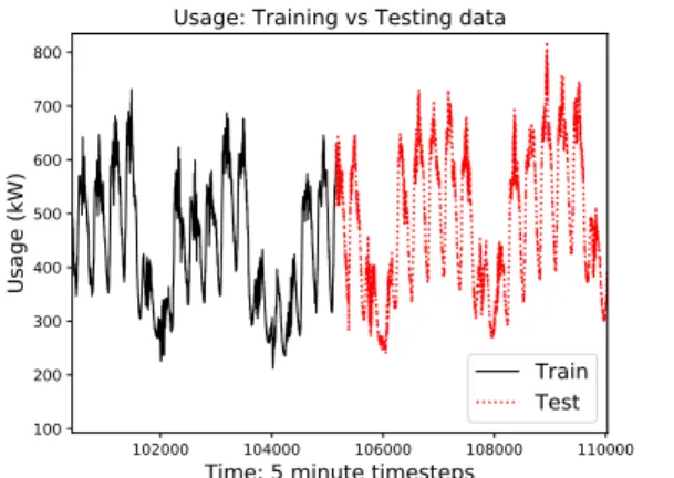
The entire dataset was divided into a training and test set. The first 80% of all readings were assigned as the training set and the last 20% as the test set. Fig. 2 shows where the train set ends and test set begins for the usage feature. This validation process was chosen since the problem is time series specific, and thus, randomizing the entire dataset prior to subsetting (splitting into train and test set) is counter intuitive; it would potentially allow the model to see the most recent energy data during training, while being tested on the first most data. Note that the usage data, as seen in Fig. 2, describes a building that experiences a regular work-week.
102000 104000 106000 108000 110000
Time: 5 minute timesteps 100 200 300 400 500 600 700 800 Usage (kW)
Usage: Training vs Testing data
Train Test
Figure 2. Usage data zoomed in to show breakdown between the train and test sets.
Hence, the spikes represent the typical Monday-Friday work-week, while the drops represent lower consumption during the weekend.
The data was normalized using standardization. Hence, the values of each feature in the data were transformed to have zero-mean and unit-variance. The formula used is given as:
˜
x=x−µ
σ (3)
Here,xis the original feature vector,µis the mean of that feature vector,σ is its standard deviation, andx˜ represents the feature vector after normalization.
B. Sample Generation
An important step of the S2S approach is the sample generation process. More specifically, how the input and target samples were generated to be passed to the model. Let one input sample be represented as a matrix,X ∈ RT×f,
whereT is the number of time steps andf is the number of features. As defined in the previous subsection, the number of features wasf = 11, where each row of the matrixX is defined as:
x[t]= [Month[t] DayOfYear[t] DayOfMonth[t]
Weekday[t] Weekend[t] Holiday[t] Hour[t]
Season[t] Temp[t] Humidity[t] Usage[t]]
(4)
Where t ∈ 1, ..., T. For each input sample, one target sample was generated, represented by a vector y ∈RN×1,
where N represents the number of predicted time steps fromT. The target vector represents the actual usage vector, which is given by:
y= [Usage[1], ... , Usage[n], ... , Usage[N]] (5) Where y[n] is the actual usage value at time stepn, and n∈1, ..., N. We use this target vector to compare with the predicted usage vector, y˙∈RN×1.
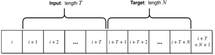
Thus, the input and target samples were generated using the technique demonstrated in Fig. 3. Here,i+ 1denotes the index (of the dataset) where the window starts, T denotes the length of the input window, and N denotes the length of the target vector. As an example, to predict the next hour of energy consumption using the previous four hours (in 5-minute increments), T and N would be set to T = 48
and N = 12. It is important to note that the indices (minus the last T +N) of the training set were first uniformly randomized, not the data itself, then the input and target samples were generated. This way, data in a single input sample represents consecutive time steps. The formal process for sample generation, of the training set, can be given as:
1) Uniformly randomize indices i. Here, i∈ 1, ..., ilast. Whereilast denotes the total length of the training set minus the last T+N indices. Ifi was chosen to be
Table I
FEATUREDATA(BEFORE STANDARDIZATION)
Index Month Day of Year Day of Month Weekday Weekend Holiday Hour Season Temp. (◦C) Humidity Usage (kW)
0 7 187 5 1 0 0 0 3 21.0 83.0 405.8743
23470 9 268 24 5 1 0 18 4 19.0 60.0 332.7853
104275 7 184 3 0 0 1 7 3 18.0 100.0 297.4848
ilast+ 1, the input sample would still be lengthT, but the target sample would now be length N −1, since it is not possible to exceed the available index of the training set.
2) For eachi:
a) Append, from the training set, consecutive data from indices i+ 1toi+T as the input sample. Hence, obtainingX ∈RT×f.
b) Append, from the training set,i+T+1toi+T+ N as the target usage vector. Hence, obtaining
y∈RN×1.
Obtaining the input and target samples for thetest setwas slightly different. Instead, as seen in Fig. 4, a sliding window technique was used; the window shifted sequentially with the overlap size equivalent to the target length, N. Hence, if we obtain one test input sample starting at index i0+ 1, the target sample still ends ati0+T+N, similar to what is
done in Fig. 3 and the training set. However, the indices are not randomized for the test set, and the next input sample slidesN time steps and starts ati0+ 1 +N, with the target sample ending ati0+T+2N. The formal process for sample generation, of the test set, can be given as:
1) For eachi0, s.t.i0 ∈1,1 +N,1 + 2N, ..., i0last, where
i0last denotes total length of the test set minus the last
T+N:
a) Append, from the test set, consecutive data from indicesi0+1toi0+Tas the input sample. Hence, obtaining X0 ∈RT×f.
b) Append, from the test set,i0+T+1toi0+T+N
as the target usage vector. Hence, obtainingy0 ∈
RN×1.
Note that the process above accounts for the sliding window technique by starting at index 1 and addingN each time. Doing so allows for an overlap in input test samples, but no overlap in target test samples. This was done to
concatenate the predicted usage vectors together into one
vector which has equivalent length as the total actual usage vector. Thus, from here, comparisons between the predicted
i i + 1 i + 2 ...
Target: length
i + T i + T + 1 i + T + 2 ... i + T + N + N + 1i + T
Input: lengthT N
Figure 3. Training set sample generation. Input and target samples generated from random indexi+ 1of the dataset.
and actual usage can be done by means of accuracy measures and plotting.
C. S2S Algorithm
This section gives a detailed breakdown of the S2S algo-rithm used for this work. As briefly described in section II, each RNN (LSTM and GRU) has an Encoder RNN (ET) of lengthT and Decoder RNN (DN) of lengthN respectively. The inputs, as obtained in the previous subsection, are passed throughET, one time step at a time. Hence, Fig. 1 (a) shows
ET unrolled, where a vector, as in (4), is passed to it at each time step. Each cell takes the previous hidden state and the current input at time t, performs the actions discussed in section II (equations 1a-f for an LSTM cell or 2a-d for a GRU cell), and outputs a hidden state. Note that GRU cells output one hidden state, while LSTM cells output both a cell state and a hidden state.
Fig. 5 shows howET andDN connect for the proposed S2S approach. Once the entire input has been processed by
ET, the output produced is a hidden state commonly referred to as the context vector [8], since it encodes context from the entire input sequence. This context vector, shown ash[T]
in Fig. 5, is then used as the initial hidden state for DN. The context vector is also passed through a fully-connected layer to produce the feature context value, shown as y˙[0],
which is the initial input of DN. Let us denote this fully-connected layer as Wh→1, where h represents the hidden state dimension, otherwise known as the number of features in the hidden state of each cell. Note that theET cell took
f = 11features as input, while theDN cell only takesf = 1 feature, hence the previously predicted usage value y˙[n−1].
Therefore, this Wh→1 transforms the output vector from
dimensionhto a single value of dimension1, allowing it to be used as the next input value forDN. Hence, this approach is novel to building-level load forecasting, and separates this work from others in literature. Thus, let us denote these proposed models with a “-o” notation, representing the distinguishing characteristic of the proposed architecture for energy load forecasting; one predicted value computed at time stepn is passed as the next input. Hence, GRU S2S will be denoted as GRU S2S-o.
Continuing, each output produced from the remainingDN cells is passed through the same fully-connected layer. This transforms the output¯h[n] to a single predicted usage value,
˙
y[n], at time step n. Thus, after N time steps we have
+ T i′ + N + 1 Input i′ i′+ 1 i′+ 2 ... Target + T i′ i′+ T + 1i′+ T + 2 ... i′+ T + N (b) Input + N i′ i′+ 1 + Ni′+ 2 + N ... i′+ T + N + 1 i+ T ′ + N + 2 ... i+ T ′ + 2N i+ T ′ + 2N + 1 Target + T + N i′ (a)
Figure 4. Test set sample generation. (a) Input and target samples generated from dataset at index i0+ 1. (b) Sequential input and target samples generated from sliding window with overlap lengthN.
the loss from the target usage vector, formally given as:
L= 1 n N X n=1 (y[n]−y˙[n])2 (6)
Where (6) is the objective function that is minimized after each epoch; it is calculated as the Mean Squared Error (MSE) of the target and predicted values.
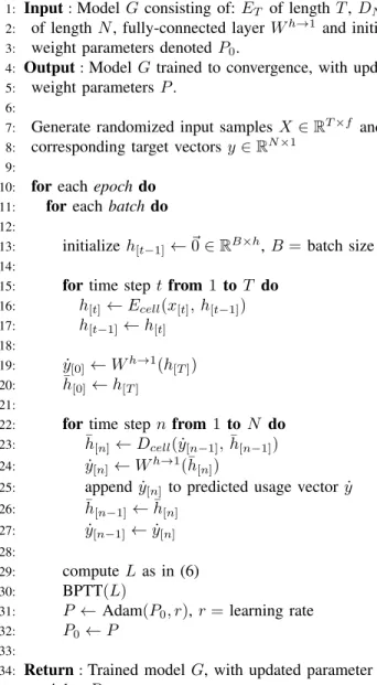
To train the model, back-propagation through time (BPTT) is used. The entire network is unrolled by a fixed number of time steps T +N; hence, it can be seen as a deep standard feed-forward neural network with shared parameters. Thus, standard BPTT can be applied to train the network using a gradient based method. Here, the ADAM [28] algorithm is used as the gradient based optimizer since it outperformed other methods in terms of faster convergence and better accuracy measures. The complete process is formally given in Algorithm 1. In step 13, we initialize the hidden state to be~0 of size B×h, where B is denoted as the batch size - the number of training examples the model processes for one update of weight parameters [29]. Batching is done to speed up convergence. Since the weight parameters are updated per batch, a smaller batch size provides a more accurate update. Once all the batches have been processed by the model, one full epoch has occurred. Steps 15-17 show the input being passed through the ET. Steps 19-20 transform the output of ET, the context, to create the initial input and hidden state of the DN. Steps 22-27 describe the process of predicting the usage value, appending that value, and preparing the next input and hidden state. In steps 29-32, the total loss is computed, BPTT is applied, and the model parameters are updated. See that Algorithm 1, Train-S2S, is used to train the model, and will differ slightly when applied to the test set. Namely, for the test set, we build the inputs and targets differently
(as outlined in the subsection IV-B) and do not apply BPTT on the loss, hence do not update the parameters in anyway.
V. EXPERIMENTS ANDRESULTS
The used dataset is based on approximately 1 year and 3 months of energy consumption data, in kW, for one commercial building/smart meter. The readings were in five minute increments, so the total number of readings was 12 readings in one hour× 24 hours in one day=287 ×458 days =131,446. As stated in section IV, each reading, or row of data, consists 11 features. The rest of this section covers the conducted experiments and their results. A. Experiments
The model was tested for three different prediction length scenarios, which we consider here as short, medium, and long prediction lengths. Since input length T to prediction length N combinations are endless, the following three
cases were chosen for experiments:
• Case 1(Short): inputT = 12, predict N = 6
• Case 2(Medium): inputT = 144, predict N = 48
• Case 3(Long): inputT = 288, predict N= 120
In 5 minute increments, those cases equate to: 1 hour
→ predicts next 30 minutes, 12 hours → predicts next 4 hours, and 24 hours →predicts next 10 hours, respectively. Although the longest length of applicable prediction is 10 hours, this length correlates to predicting 120 time steps. With datasets consisting of one-hour increments, 120 time steps would translate to predicting 120 hours (5 days) consecutively.
No model was trained for longer than 10 epochs, and the hyperparameters were kept the same for each respective model, and for each case. In all experiments, 10 epochs was sufficient to reach an acceptable level of convergence. The total loss computed, for both the training and test set, showed minimal signs of improvement as the 10th epoch approached. These precautions were taken to observe and compare each model’s performance fairly and reasonably in
ECell x[T] Wh→1 y˙[0] h[T] DCell Wh→1 y˙[1] h¯[1] DCell Wh→1 h¯[2] y˙[2] ECell x[T−1] h[T−1] Decoder ... ... ET DN Encoder
Figure 5. Detailed process of the S2S RNN. The left box shows the last two steps ofET, while the right box shows the first two steps ofDN.
Algorithm 1 Train-S2S(G= (ET, DN, Wh→1, P0))
1: Input:ModelGconsisting of:ET of lengthT,DN
2: of lengthN, fully-connected layerWh→1 and initial 3: weight parameters denotedP0.
4: Output:Model Gtrained to convergence, with updated
5: weight parameters P. 6:
7: Generate randomized input samplesX ∈RT×f and
8: corresponding target vectorsy∈RN×1
9:
10: foreach epochdo
11: foreachbatchdo
12:
13: initializeh[t−1]←~0∈RB×h,B =batch size
14:
15: fortime step tfrom 1 to T do
16: h[t]←Ecell(x[t], h[t−1]) 17: h[t−1] ←h[t] 18: 19: y˙[0]←Wh→1(h[T]) 20: ¯h[0]←h[T] 21:
22: fortime step nfrom 1 to N do
23: ¯h[n]←Dcell( ˙y[n−1],¯h[n−1]) 24: y˙[n]←Wh→1(¯h[n])
25: appendy˙[n] to predicted usage vectory˙ 26: ¯h[n−1] ←¯h[n]
27: y˙[n−1]←y˙[n] 28:
29: computeL as in (6) 30: BPTT(L)
31: P← Adam(P0, r),r=learning rate 32: P0←P
33:
34: Return:Trained modelG, with updated parameter
35: weights P.
terms of accuracy. The hyperparameters used to compute the results were:
• Hidden dimension sizeh= 64
• Cell state dimension sizec= 64(only for LSTM) • Batch size = 256
• Epochs = 10
• Learning rate = 0.001
Note that choosing these external parameters has yet to be optimized, and doing so holds potential for improved results. The S2S-o models with GRU/LSTM cells were compared against a S2S-o model with the basic RNN cell, as well as a Deep Neural Network, for all three cases. The DNN took the same input matrix X ∈ RT×f, but instead flattened it into a single vector of dimension size = T ×f. This vector was then passed through three deep layers consisting of512nodes per layer. The output was a layer consisting of
N nodes, which is equivalent to lengthN of the predicted usage sequence used in the S2S-o models. The DNN is used to directly predict the sequence of values, all at once, while the S2S-o models sequentially predict the values one at a time. Thus, the DNN results give a good comparison be-tween direct prediction accuracy versus sequential prediction accuracy. The activation function used for the output layer was linear, since this is a regression problem.
As stated in the sample generation subsection, there was no overlap in target test samples, to enable concatenation of predicted usage vectors into one vector. Hence, the accuracy measures were obtained by comparing this one overall pre-dicted usage vector against the overall actual usage vector. The accuracy measures used throughout this work were the Mean Absolute Error (MAE) and Mean Absolute Percentage Error (MAPE), given by the following equations:
MAE= 1 n n X i=0 |yi−yˆi| (7) MAPE= 100% n n X i=0 yi−yˆi yi (8) Whereyrepresents the actual value,yˆthe predicted value, and number of observations or samples is given byn.
Lastly, since this work randomized the training samples, it was important to run a few simulations where the model saw a different randomized order of training samples each time. Hence,7 random seeds were used for each case. For example, if random seed equals 1, then the training samples are in one randomized order, and that order is used by each model, for that case. If random seed equals 2, the training samples are in a different randomized order. A value (such as 1 or 2) is assigned to the seed to keep track of the random order, to later reproduce identical results.
B. Results and Discussion
The results were computed using Python and the PyTorch optimized tensor library [30], which is an open-source machine learning library.
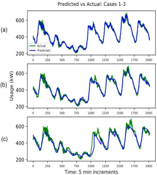
Fig. 6 shows the predicted usage values obtained from the GRU S2S-o model compared to the actual, for all three cases. Each plot shows only the last 7 days of the test set, and it was produced with the same external parameters for each case. From Fig. 6, we can observe that the accuracy decreases as we move from Case 1 → 3. Hence, Fig. 6 (a) shows the predicted values best fitting to the actual values, with 6 (b) showing lower accuracy and 6 (c) showing the worst. Hence, as the prediction lengthN increases, the accuracy is expected to decrease [15] [16]. This can also be seen in Table II, which gives the accuracy that each model obtained in terms of MAE and MAPE for all three cases. A visualization of the MAPE increasing from Case 1→ 3 is demonstrated in Fig. 7.
0 250 500 750 1000 1250 1500 1750 2000
200
400
600
Actual Predicted 0 250 500 750 1000 1250 1500 1750 2000200
400
600
Usage (kW) 0 250 500 750 1000 1250 1500 1750 2000Time: 5 min increments
200
400
600
Predicted vs Actual: Cases 1-3
(b)
(c) (a)
Figure 6. Predicted usage compared to actual, for the three cases: Hence, (a) represents case 1, (b) and (c) represent cases 2 and 3 respectively.
Therefore, as seen in Table II and Fig. 7, even though ac-curacy does decrease for the GRU/LSTM S2S-o models, it is clear they still outperform the RNN S2S-o and DNN model, for all three forecasting cases. As expected, the GRU/LSTM S2S-o models significantly outperformed the basic RNN S2S-o model for longer prediction horizon represented with case 3. This was expected as LSTM and GRU cells were introduced to overcome the long-term drawbacks that RNN cells pose.
It is interesting to compare the results between the GRU S2S-o and LSTM S2S-o models. For cases 1 and 2, the results are very similar. For case 3, the GRU S2S-o model outperformed the LSTM S2S-o model, with 12.56% de-crease in MAE and 14.05% dede-crease in MAPE. Section II provides a detailed analysis of calculations occurring in an LSTM and GRU cell respectively. The LSTM cell contains an extra secondary state, called the cell state, as well as an extra gate. Even though the GRU cells have fewer states, they outperformed the LSTM cells. This result is similarly
Case 1 Case 2 Case 3
2 3 4 5 6 7 8 MAPE (%)
MAPE (%) for Cases 1-3 GRU S2S-o
LSTM S2S-o RNN S2S-o DNN
Figure 7. MAPE (%) for the three cases and for each model. confirmed by Chunget al. [31] and Jozefowiczet al. [32].
VI. CONCLUSION
The rapid expansion of high-density cities along with accompanying industrial and commercial development result in increasing energy consumption. To reduce the energy footprint, it is crucial to enhance energy management strate-gies for buildings; energy forecasting is an important aspect of such initiatives. Sensor-based energy forecasting uses historical data from smart meters or other sensors to predict energy consumption. This study belongs to sensor-based forecasting category; it uses data from smart meters and deep learning algorithms to predict energy consumption. A novel methodology in both sample generation and S2S RNN algorithm for building-level energy forecasting is proposed. Hence, this work adapts a true S2S approach from language translation for energy load forecasting: the predicted output value is passed as the next input in the decoder. The method-ology was applied to three S2S RNN cell-based models: basic RNN, GRU, and LSTM. All were trained and tested on five minute incremental data, with equivalent external parameters, and compared against a Deep Neural Network. The GRU S2S-o and LSTM S2S-o models outperformed the basic RNN S2S-o and DNN models, for short, medium, and long-term prediction lengths. On average, the GRU S2S-o model outperformed the LSTM S2S-o model, for all three prediction lengths.
Table II
ACCURACY RESULTS FOR THE ALL MODELS AND ALL CASES. TOP NUMBER IS BEST ACHIEVED;NUMBER IN BRACKETS IS THE AVERAGE OF RUNS.
Model MAE MAPE (%)
Case 1 Case 2 Case 3 Case 1 Case 2 Case 3
GRU S2S-o 10.673 18.432 24.378 2.365 4.137 5.416 (10.946) (19.369) (26.037) (2.441) (4.363) (5.834) LSTM S2S-o 10.736 18.491 27.441 2.381 4.136 6.178 (11.029) (21.161) (29.745) (2.451) (4.745) (6.695) RNN S2S-o 10.908 21.584 84.729 2.440 4.992 18.950 (11.196) (43.000) (99.994) (2.510) (10.233) (23.698) DNN 12.258 25.681 28.40 2.733 6.082 6.777 (12.487) (28.845) (29.486) (2.826) (6.898) (7.041)
Future work will analyze the GRU o and LSTM S2S-o mS2S-odel S2S-outcS2S-omes fS2S-or lS2S-onger-term predictiS2S-on, and apply the S2S-o algorithm to relatable datasets.
ACKNOWLEDGMENT
The authors would like to thank Utilismart Corporation for supplying industry knowledge and data used in this study.
REFERENCES
[1] H. Ritchie and M. Roser, “Urbanization,” 2018, Our World in Data, Available: https://ourworldindata.org/urbanization. [Ac-cessed: Jan. 2019].
[2] U.S. Energy Information Administration, “Use of En-ergy in the United States Explained,” 2017, Available: https://www.eia.gov/energyexplained. [Accessed: Jan. 2019]. [3] H. C. Akdag and T. Beldek, “Waste Management in Green
Building Operations Using GSCM,”International Journal of Supply Chain Management, Vol. 6 (3), pp. 174–180, 2017.
[4] Independent Electricity System Operator, “Global
Adjustment and Peak Demand Factor,” 2019, Available: http://www.ieso.ca/Sector-Participants/Settlements/Global-Adjustment-and-Peak-Demand-Factor. [Accessed: Jan. 2019] [5] J. Schmidhuber, “Deep learning in neural networks: an
overview,”Neural Networks, Vol. 61, pp. 85–117, 2015. [6] D. E. Rumelhart, G. E. Hinton and R. J. Williams, “Learning
representations by back-propagating errors,”Nature, Vol. 323 (6088), pp. 533–536, 1986.
[7] A. Graves, S. Fernandez, F. Gomez and J. Schmidhuber, “Connectionist temporal classification: labelling unsegmented sequence data with recurrent neural networks,” InProc. of the International Conference on Machine Learning (ICML), pp. 369–376, 2006.
[8] I. Sutskever, O. Vinyals and Q. V. Le, “Sequence to sequence learning with neural networks,” InProc. of Advances in Neural Information Processing Systems (NIPS), pp. 3104–3112, 2014. [9] G. E. Dahl, D. Yu, L. Deng, and A. Acero, “Context-dependent pre-trained deep neural networks for large-vocabulary speech recognition,” IEEE Transaction on Audio, Speech, and Lan-guage Processing, Vol. 20 (1), pp. 30–42, 2012.
[10] A. Krizhevsky, I. Sutskever, and G. E. Hinton, “ImageNet classification with deep convolutional neural networks,” In Proc. of Advances in Neural Information Processing Systems (NIPS), pp. 1097–1105, 2012.
[11] P. J. Werbos, “Backpropagation through time: what it does and how to do it,”Proceedings of the IEEE, Vol. 78 (10), pp. 1550–1560, 1990.
[12] R. Pascanu, T. Mikolov, and Y. Bengio, “On the difficulty of training recurrent neural networks,” In Proc. of the Inter-national Conference on Machine Learning (ICML), pp. 1310– 1318, 2012.
[13] S. Hochreiter and J. Schmidhuber, “Long short-term mem-ory,”Neural Computation, Vol. 9 (8), pp. 1735–1780, 1997. [14] K. Choet al., “Learning phrase representations using RNN
encoder–decoder for statistical machine translation,” In Proc. of the Empirical Methods in Natural Language Processing (EMNLP), pp. 1724–1734, 2014.
[15] D. L. Marino, K. Amarasinghe and M. Manic, “Building energy load forecasting using deep neural networks,” InProc. of the IEEE Industrial Electronics Society (IECON), pp. 7046– 7051, 2016.
[16] E. Mocanu, P. H. Nguyen, M. Gibescu and W. L. Kling, “Deep learning for estimating building energy consumption,” Sustainable Energy, Grids and Networks, Vol. 6 (1), pp. 91–99, 2016.
[17] J. G. Jetcheva, M. Majidpour and W. Chen, “Neural network model ensembles for building-level electricity load forecasts,” Energy and Buildings, Vol. 84 (1), pp. 214–223, 2014. [18] S. Ferlito et al., “Predictive models for building’s energy
consumption: an artificial neural network (ANN) approach,” In Proc. of the Italian Association of Sensors and Microsystems (AISEM), pp. 1–4, 2015.
[19] Y. T. Chae, R. Horesh, Y. Hwang, and Y. M. Lee, “Artificial neural network model for forecasting sub-hourly electricity usage in commercial buildings,” Energy and Buildings, Vol. 111 (1), pp. 184–194, 2016.
[20] S. Najiet al., “Estimating building energy consumption using extreme learning machine method,” Energy, Vol. 97 (1), pp. 506–516, 2016.
[21] D. B. Araya, K. Grolinger, H.F. ElYamany, M. Capretz and G. Bitsuamlak, “An ensemble learning framework for anomaly detection in building energy consumption,” Energy and Buildings, Vol. 144 (1), pp. 191–206, 2017.
[22] S. Seyedzadeh, F. P. Rahimian, I. Glesk and M. Roper, “Ma-chine learning for estimation of building energy consumption and performance: a review,”Visualization in Engineering, Vol. 6 (1), pp. 5–25, 2018.
[23] N. L. Tasfi, W. A. Higashino, K. Grolinger and M. A. Capretz, “Deep neural networks with confidence sampling for electrical anomaly detection,” InProc. of the IEEE International Con-ference on Smart Data, pp. 1038–1045, 2017.
[24] K. Amarasinghe, D. L. Marino and M. Manic, “Deep neural networks for energy load forecasting,” In Proc. of the IEEE International Symposium on Industrial Electronics (ISIE), pp. 1483–1488, 2017.
[25] P. Malhotra, L. Vig, G. Shroff and P. Agarwal, “Long short term memory networks for anomaly detection in time series,” In Proc. of the European Symposium on Artificial Neural Networks, Computational Intelligence and Machine Learning (ESANN), pp. 89–95, 2015.
[26] S. Bouktif, A. Fiaz, A. Ouni and M. A. Serhani, “Optimal deep learning LSTM model for electric load forecasting us-ing feature selection and genetic algorithm: comparison with machine learning approaches,”Energies, Vol. 11 (7), pp. 1636– 1656, 2018.
[27] Weather Underground, “Historical Weather,” 2018, Avail-able: https://www.wunderground.com/history. [Accessed: May 2018]
[28] D. P. Kingma and J. Ba, “Adam: a method for stochastic optimization,”arXiv preprint arXiv:1412.6980, 2014. [29] E. Hoffer, I. Hubara and D. Soudry, “Train longer, generalize
better: closing the generalization gap in large batch training of neural networks,” InProc. of Advances in Neural Information Processing Systems (NIPS), pp. 1731–1741, 2017.
[30] A. Paszke, S. Gross, S. Chintala, and G. Chanan, “Py-Torch: from research to production,” 2016. Available: https://pytorch.org. [Accessed: May, 2018]
[31] J. Chung, C. Gulcehre, K. Cho and Y. Bengio, “Emperical evaluation of gated recurrent neural networks on sequence modeling,”arXiv preprint arXiv:1412.3555, 2014.
[32] R. Jozefowicz, W. Zaremba, and I. Sutskever, “An emperical exploration of recurrent network architectures,” InProc. of the International Conference on Machine Learning (ICML), pp. 2342–2350, 2015.
![Figure 1. Sample passed through the RNN S2S network. Here, ~ c and ˙ y [0]](https://thumb-us.123doks.com/thumbv2/123dok_us/10013546.2493685/3.918.471.834.110.219/figure-sample-passed-rnn-s-s-network-c.webp)