Effect of Different Distance Measures in
Result of Cluster Analysis
Master’s Thesis
Aalto University School of Engineering,
Department of Real Estate, Planning and
Geoinformatics,
Date: 04.08.2015
Sujan Dahal
Degree Program in Geomatics
Supervisor: Professor Kirsi Virrantaus
Instructor: D.Sc.(Tech) Jussi Nikander
In Loving Memory Of My Grandmother
Dhana Laxmi Tripathee
Aalto University, P.O. BOX 11000, 00076 AALTO www.aalto.fi Abstract of master's thesis
Author Sujan Dahal
Title of thesis Effect of Different Distance Measures in Result of Cluster Analysis Degree programme Geomatics
Major/minorGeoinformatics Code M3002
Thesis supervisorProf. Kirsi-Kanerva Virrantaus, Department of Real Estate, Planning and
Geoinformatics, Aalto University.
Thesis advisor(s) D.Sc. (Tech)Jussi Nikander, Principal Research Scientist, Natural Resources
Institute Finland
Date 04.08.2015 Number of pages77 Language English
Abstract
The objective of this master’s thesis was to explore different distance measures that could be used in clustering and to evaluate how different distance measures in K-medoid clustering method would affect the clustering output. The different distance measures used in this research includes Euclidean, Squared Euclidean, Manhattan, Chebyshev and Mahalanobis distance. To achieve the research objective, K-medoid method with different distance measures was applied to a spatial dataset to explore relative information revealed by each distance measure. The effect of each distance measure on output is documented and the output was further compared with each other to reveal the differences between each distance measure.
The study starts with literature review of cluster analysis process where necessary steps for performing cluster analysis are explained. In literature section, different clustering methods with particular characteristics of each method are described that would serve as basis for choice of clustering method. Data description and data analysis is included thereafter which is followed by interpretation of clustering result and its use for Terrain analysis. Terrain analysis has its significance in forest industry, military as well as crisis management and is usually concerned with off-road mobility of a vehicle or a group of vehicles between given locations. In case of terrain analysis, clustering could be used to group the similar areas and determine the off-road mobility of a particular vehicle. This result could be further categorized according to suitability of the item in the cluster and interpreted using expert evaluation in order to reveal useful information about mobility in a terrain.
Cluster Validation measures were applied to output of clustering to determine the differences between different distance measures. The findings of this study indicate that in the study area, there exists some level of differences in the result of clustering when different distance measures are used. This difference is then interpreted with the help of input dataset and expert opinion to understand the effect of different distance measures in the dataset. Finally, the study provides basis for mobility analysis with help of clustering output.
Keywords Spatial Analysis, Clustering, Similarity Measures, Distance Measures, K-medoid
Table of Contents
LIST OF ABBREVIATIONS ... III LIST OF FIGURES ... IV LIST OF TABLES ... VI
1. INTRODUCTION ... 1
1.1 THESIS STRUCTURE ... 4
1.2 RELATED WORKS ... 4
1.3 OBJECTIVES OF RESEARCH AND RESEARCH QUESTIONS ... 7
1.4 MOBILITY ANALYSIS ... 8
1.5 METHODS AND MATERIALS ... 10
2 CLUSTER ANALYSIS ... 11
2.1 APPLICATION AND OBJECTIVE OF CLUSTER ANALYSIS ... 12
2.2 WORK FLOW IN CLUSTER ANALYSIS ... 13
2.3 ASSUMPTIONS IN CLUSTER ANALYSIS ... 15
2.4 CLUSTERS ANALYSIS AS MEASURE OF SIMILARITY ... 15
2.5 DISTANCE MEASURES ... 16
2.6 MINKOWSKI DISTANCE ... 17
2.6.1 Euclidean Distance ... 19
2.6.2 Squared Euclidean Distance ... 20
2.6.3 Manhattan Distance ... 21
2.6.4 Chebyshev Distance ... 22
2.7 MAHALANOBIS DISTANCE ... 24
2.8 SELECTING THE BEST DISTANCE MEASURE ... 25
2.9 CLUSTERING METHODS ... 26
2.9.1 Partitioning Methods ... 26
2.9.2 Hierarchical Methods ... 32
2.9.3 Density Based Methods ... 34
2.9.4 Grid Based Methods ... 36
2.9.5 Fuzzy Clustering ... 37
2.10 NUMBER OF CLUSTERS AND HETEROGENEITY MEASUREMENT ... 37
2.11 DATA STANDARDIZATION ... 38
2.12 CLUSTER VALIDATION ... 39
3 DATA ANALYSIS ... 43
3.1 ANALYSIS DESIGN ... 43
3.2 STUDY AREA AND DATA DESCRIPTION ... 45
3.3 DATA EXPLORATION ... 46
3.4 COMPUTATIONAL ANALYSIS ... 48
4 RESULT INTERPRETATION ... 50
4.1 CLUSTER MAP ... 50
4.2 CLUSTER VALIDATION ... 55
4.2.1 Misclassification Matrix and Visual Analysis ... 55
4.2.2 Cluster Validation ... 66 5 DISCUSSION ... 68 5.1 CHALLENGES ... 70 5.2 FUTURE RESEARCH ... 71 6 CONCLUSION ... 72 REFERENCES ... 74 APPENDIX 1 ... A APPENDIX 2 ... B APPENDIX 3 ... C
LIST OF ABBREVIATIONS
KDD Knowledge Discovery in Database
CLARA Clustering Large Application
CLARANS Clustering Large Applications based on Randomized Search
AGNES Agglomerative Nesting
DIANA Divisive Analysis
DBSCAN Density Based Spatial Clustering of Application with Noise
OPTICS Ordering Points to Identify the Clustering Structure
DENCLUE Density-based Clustering
STING Statistical Information Grid-based method
DEM Digital Elevation Model
LIST OF FIGURES
Figure 1 Different steps in knowledge discovery process (University of Florida, 2015)2
Figure 2 Different Steps in Cluster Analysis (Halkidi et al., 2001) ... 13
Figure 3 Different forms of Minkowski distance ... 18
Figure 4 Unit circles with various values of 'p' ... 18
Figure 5 Euclidean distance between two points ... 19
Figure 6 The local pattern of a Manhattan network and real life examples of orthogonal streets of Manhattan and Barcelona (Dalfo et al., 2007) ... 21
Figure 7 Manhattan distance (red); equivalent Manhattan distance (yellow and blue) and Euclidean distance (green) between two points (Wiktionary, 2013) ... 21
Figure 8 Chebyshev distance between two points ... 22
Figure 9 Unit Circle representation of Chebyshev distance ... 23
Figure 10 Comparison between Euclidean distance and Mahalanobis distance (Maesschalck et al., 2000) ... 24
Figure 11 K-Means clustering algorithm steps (Miller & Han, 2001) ... 27
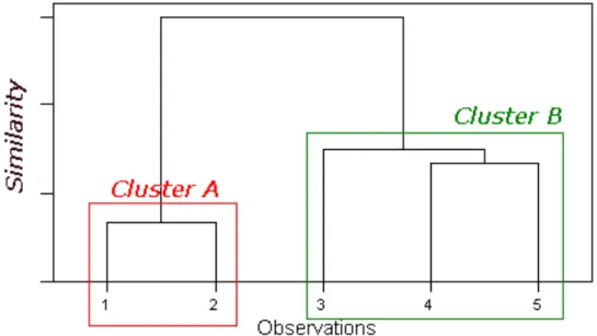
Figure 12 A dendrogram showing two distinct clusters (Manchester Metropoliton University, ) ... 32
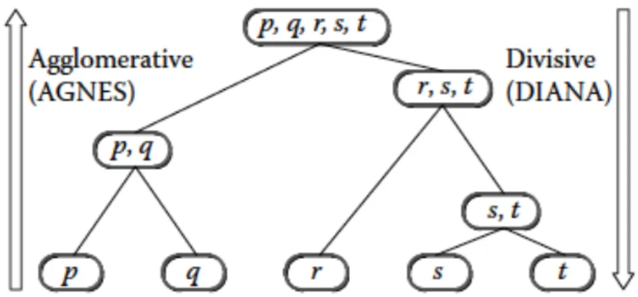
Figure 13 Agglomerative and Divisive Clustering on a set of data object (p,q,r,s,t) (Miller & Han, 2001) ... 34
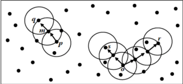
Figure 14 DBSCAN method and cluster detection (Miller & Han, 2001) ... 35
Figure 15 Grid Based Clustering (Patentdocs, 2011) ... 36
Figure 16 Workflow of Analysis Process ... 43
Figure 17 Vegetation, Soil Type and Slope raster layers ... 46
Figure 18 Normalized Slope Layer ... 47
Figure 21 Normalized Soil Type Layer ... 48
Figure 22 Cluster map created using Euclidean distance ... 51
Figure 23 Cluster map created using squared Euclidean distance ... 51
Figure 24 Cluster map created using Manhattan distance ... 52
Figure 25 Cluster map created using Mahalanobis distance ... 52
Figure 26 Cluster map created using Chebyshev distance ... 53
Figure 27 Difference between clusters created using different distance measures. (a) Between Euclidean and squared Euclidean distance and (b) Between Euclidean and Manhattan distance. ... 57
Figure 28 Difference between clusters created using different distance measures. (a) Between Euclidean and Mahalanobis distance and (b) Between Euclidean and Chebyshev distance. ... 59 Figure 29 Difference between clusters created using squared Euclidean and Manhattan distance ... 60 Figure 30 Difference between clusters created using different distance measures. (a) Between squared Euclidean and Mahalanobis distance and (b) Between squared Euclidean and Chebyshev distance. ... 62 Figure 31 Difference between clusters created using different distance measures. (a) Between Manhattan and Mahalanobis distance and (b) Between Manhattan and Chebyshev distance. ... 64 Figure 32 Difference between clusters created by Mahalanobis and Chebyshev distance. ... 65
LIST OF TABLES
Table 1 Misclassification Matrix of Euclidean and Squared Euclidean Distance ... 56 Table 2 Misclassification Matrix of Euclidean Distance and Manhattan Distance ... 57 Table 3 Misclassification Matrix of Euclidean Distance and Mahalanobis Distance .. 58 Table 4 Misclassification Matrix of Euclidean Distance and Chebyshev Distance .... 58 Table 5 Misclassification Matrix of Squared Euclidean Distance and Manhattan Distance ... 60 Table 6 Misclassification Matrix of Squared Euclidean Distance and Mahalanobis Distance ... 61 Table 7 Misclassification Matrix of Squared Euclidean Distance and Chebyshev Distance ... 61 Table 8 Misclassification Matrix of Manhattan Distance and Mahalanobis Distance 63 Table 9 Misclassification Matrix of Manhattan Distance and Chebyshev Distance ... 63 Table 10 Misclassification Matrix of Mahalanobis Distance and Chebyshev Distance64 Table 11 Comparison of external indices for different distance measures ... 66
1. Introduction
Recent advancements in data acquisition and storage technologies have resulted in growth of huge databases. This advancement ranges in different areas from credit card usage data, telephone call data, government statistics, astronomical data, molecular database as well as geographic databases
(Hand et al., 2001). Research in the field of medicine, science and engineering are rapidly accumulating data that is key to important new discoveries. This progress has been induced by the fact that systems are often been used in different fields that we do not know in depth and need more information about them. This lack of knowledge should be compensated by the mass of the stored data that is available nowadays. The available data have induced the need to process and use it. The data reflects the behavior of the analyzed system; therefore there is a theoretical potential to obtain useful information
and knowledge from the data (Abonyi & Feil, 2000). However, extracting
useful information from available dataset is extremely challenging. Often, traditional data analysis methods, which are based on hypothesize-and-test paradigm, cannot be used because of size of data. Also, non-traditional nature of data means that traditional approaches cannot be applied even if the dataset is relatively small. Most of non-traditional methods are motivated by the desire to automate the process of hypothesis generation and its evaluation. Further, there can be situations where questions that need to be answered cannot be addressed using existing data analysis techniques thus, new methods are required to be used in order to extract useful information
from huge datasets (Tan et al., 2006).
One of the areas of advancement in data acquisition is in the field of geography where advancement in data collection methods like photogrammetry and remote sensing has led to acquisition of huge amount of data. Thus, geography has moved towards data-rich and computation –rich environment. The scope, coverage, and volume of geographic datasets are rapidly growing. Geographical data are unique in nature due to special characteristics such as geographic measurement framework, spatial autocorrelation, heterogeneity, complexity of spatial objects and relationships
and diversity of data. So, it requires unique tools for analysis and provides unique research challenge. Formal and computational representation of the geographic information requires adoption of implied topological and geometric measurement framework, which affects measurement of geographic attributes and consequently the patterns that can be extracted. Thus, because of inductive nature and ability to handle heterogeneous datasets,
data mining is appropriate tool for exploring geographical databases. (Miller
& Han, 2001)
Data mining is the analysis of large observational data sets to find unsuspected relationships and to summarize the data in novel ways that are both understandable and useful to the data owner. Data mining is often set in
broader context of Knowledge Discovery in Database (KDD). The KDD
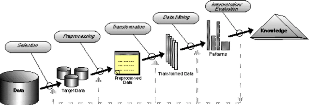
process involves different stages: selecting the target data, preprocessing the data, transforming if necessary, data mining to extract patterns and relationships, and finally interpreting and assessing the discovered structures.
(Hand et al., 2001)
Figure 1 Different steps in knowledge discovery process (University of Florida, 2015)
The extraction of information is useful for understanding the overall knowledge discovery process. There are different possible ways to extract patterns and determine relationships in the dataset. Clustering is partition of a dataset into subsets so that the data in each subset shares some common trait. (Abonyi & Feil, 2000)
Clustering is one of the most primitive mental activities of humans, used to handle huge amount of information we receive everyday. Processing every piece of information as a single entity would be impossible. Thus, humans
tend to categorize entities into clusters where each cluster is characterized by
common attributes of the entities it contains. (Theodoridis & Koutroumbas ,
2003). Mostly cluster analysis reveals meaningful groups in data, revealing natural structure of the data. For understanding the dataset, cluster analysis has an important role in wide variety of fields like psychology, social sciences, biology, statistics, pattern recognition, information retrieval, geosciences and
many more. (Tan et al., 2006)
Most of the geographical datasets are multivariate in nature and contains different attributes as well as geographic information. To reveal important patterns from such dataset is a challenging task as the patterns may have various forms (linear or nonlinear) and involve multiple spaces (e.g. multi-variate space and geographic space). To be considered as a multimulti-variate data, all the variables must be random and interrelated in such ways that their different effects cannot meaningfully be interpreted separately. Thus, multivariate analysis techniques are applied to such dataset to analyze
multiple variables in a single relationship or a set of relationships. (Hair et al.,
2006)
There are different forms of geographic data of which, point data is the simplest form. The location of a spatial object or an event is represented as a point. In the case of clustering, point data is generally used to calculate
distance between data objects.Distance is one of the widely used measures
in the process of spatial analysis. Especially, in clustering, to determine the clusters, distance is one of the important parameter. The goal of clustering is to find clusters from unlabeled data so that the data element that belongs to same clusters is as similar as possible whereas data belonging to different clusters are as dissimilar as possible. It is one of the main exploratory data analysis methods where similar items are grouped as close as possible. Distance measures can be then applied to compute the similarity between objects. (Miller & Han, 2001)
Similarity represents the degree of correspondence among objects across all
of the characteristics used in the analysis. (Hair et al., 2006). Similarity enables
each observation to be compared to each other and determine the objects
that are similar to each other according to certain criteria. The term proximity
dissimilarity (Hand et al., 2001). The term ‘distance-similarity metaphor’ (Montello et al., 2003) is often used to relate distance measure with similarity
and is reminiscent of Tobler’s ‘First Law of Geography’ (Tobler, 1970). Tobler’s
first law of geography contends that one can predict the similarity of geographic features based on their distance to other features on the Earth’s surface. Thus, distance is correlated with similarity, in most cases because
distance determines similarity (Fabrikant & Montello, 2008).
The research will analyze different distance methods used for multivariate data specially focusing on using similarity measures in clustering and determine the corresponding effect on result.
1.1 Thesis Structure
The thesis consists of three distinct parts: introduction, theoretical background and data analysis.
Initially, background information about the cluster analysis and related works in field of cluster analysis is presented. Further, research question for analysis is purposed and methods and materials used in the research are defined. In second part, theoretical background related to clustering methods along with its applications and validity measures are presented. This chapter incorporates all the concepts and methods used throughout the thesis. Furthermore, the application of clustering in this research is explained.
Further, third part, Data analysis, explores the characteristics of dataset and aims to understand the dataset. This chapter deals with formulation of analysis process, application of clustering method in the dataset along with result analysis and comparison between results.
Finally, conclusion and discussion along with future works in relation to this research is presented.
1.2 Related works
The notion of proximity is fundamental component of any comprehensive
ontology of space (Worboys, 2001). The proximity of objects with a number of
attributes is typically defined by combining the proximities of individual
attribute (Tan et al., 2006). The attributes could be used to assess similarity of
(Mcintosh & Yuan, 2005), to obtain optimal values of performance parameters, or to calculate class centroids for interpretation of similarities and differences
between classes (Gorsevski et al., 2005). There has been a lot of research in
the field of clustering and different similarity measures (Worboys, 2001;
Fabrikant & Montello, 2008; Morales-Esteban et al., 2014; Pollard, 1981). However, there have been very limited comparisons between different distance measures used for clustering and its impact on result is still a subject of research. Most of the previous research is particularly focused on individual
similarity measures (Fabrikant & Montello, 2008) and its application in
clustering.
means is a very well known and relatively simple clustering method.
K-means divides a set of data items into k clusters, where the number of
clusters must be provided beforehand (Miller & Han, 2001). Each item belongs
to the cluster with nearest mean. K-means has its use in different field like
medical (Wilmer et al., 2008), spatial (Morales-Esteban et al., 2014; Borruso, 2008)
and many other fields. Typically, K-means clustering method uses Euclidean
distance to determine k number of clusters (Wilmer et al., 2008). There has
been research on use of Mahalanobis distance (Morales-Esteban et al., 2014),
as well as research on comparison between distance measures (Dong et al.,
2013) in relation to optimization of parameters in k-means.
K-Medoids is another clustering method where, the dataset of n object is
clustered with K number of clusters provided by the user. K-medoids method
is the modified form of means method. Unlike means method, in K-medoids method, instead of calculating the mean values of the objects in a cluster as reference point, actual object from the data also called as medoid is selected to represent the cluster (Miller & Han, 2001). K-medoids has its
application in computer science (Alarcon-Aquino et al., 2014), (Park & Jun,
2009), geo science (Ding et al., 2009), medicine (Zadegan et al., 2013) and other different fields. Kaufman and Rousseeuw, (1990), developed a new partitioning algorithm PAM (Partitioning Around Medoids) which used K-medoid method, to overcome the drawbacks of K-means method and create cluster with the help of medoid. Adnan et al., (2010) has presented comparison between efficiency of K-medoid method over K-means method in large multidimensional spatial data. Similar to K-means method, different
distance measures could be incorporated with K-medoid method. Jung et al., (2013) has used modified Hausdorff distance, a pattern based distance, with K-medoid clustering method for image-based scenario modeling of fractured reservoirs for flow uncertainty quantification. Also, Alarcon-Aquino et al., (2014) analyzed Minkowski distance with K-medoid method. However, comparison between different distance measures with K-medoid method is a subject of research.
One of the related applications of similarity used in this research is mobility analysis. Mobility analysis is the process of analyzing the off-road mobility of vehicle with the goal to create a map representing how difficult it is for a specified vehicle to advance over terrain. Mobility analysis has application in crisis management, military movement as well as other various areas. The goal of mobility analysis is to create a mobility map, which is a type of cost surface, where the value of each pixel represents the amount of resources required for specific activity at the location that depicts the maneuverability of the terrain in the operational area. To analyze the mobility, the cluster produced could be categorized into good or bad mobility by assigning a mobility value to each cluster which corresponds to similarity in location and
hence, similarity measures can be used for solving the problem (Nikander et
al., 2012; Nikander, 2012).
There are also many clustering methods used in field of Geoinformatics
(Miller & Han, 2001; Theodoridis & Koutroumbas , 2003; Park & Jun, 2009; Pollard, 1981; Zhai et al., 2014; Kaufman & Rousseeuw, 1990). However, most of them are focused on using standard distance measure to create clusters.
In this research, the concept of similarity is determined with the help of attribute values of the object and is used to analyze and compare different similarity measures. This research focuses on clustering with use of different distance measures and evaluates different distances for determining similarity between data objects. Further, application of different distance measures on K-Medoids clustering and affect of similarity measures on a dataset is analyzed, the result of which can be used to analyze mobility on a given terrain.
1.3 Objectives of Research and Research Questions
The thesis is based on idea that knowing different distance measures and its use on clustering would provide good insight to result interpretation of the clustering and subsequently reveal interesting knowledge about the dataset.
The main research question answered by this research is “What are different
distance measures used in clustering?” The research analyzes the different
distance measures and provides answer to “How the use of different distance
measures affects the result of spatial analysis in clustering?“ Further, the
research will also provide insight into “Which distance measures would
provide the best result in case of clustering?” Also, the research will provide
an answer to “Can a distance measure provide proper insight about similarity
of the cluster and reveal useful information?” The thesis aim to evaluate different distance measures by applying the K-medoid method to a dataset and explore the relative information revealed through each distance measures.
The objective of the research is to perform literature review about clustering methods that uses distance as important input parameter. This is followed by explanation and use of different distance measure in clustering. Further, different distance measures are then applied to the available dataset for evaluating difference/similarity and corresponding difference/similarity is documented and compared. Different distances to be used in research
include Mahalanobis distance and Minkowski distance, whose extension
includes Euclidean distance, Squared Euclidean distance, Chebyshev
distance and Manhattan Distance.
This research is an extension into similar research on mobility analysis by Nikander et.al. (2012), performed in Aalto University and provides insight on use of different distance measures for clustering which is further used for mobility analysis of given terrain.
In addition, the research has similar limitations as research performed by Nikander et.al, (2012). Here, the research is limited to spatial problems where input data can be transformed into a format where there are no explicit spatial dependencies between locations. Thus, the knowledge and information about spatial correlation between layers, as well as spatial autocorrelation between locations is not explicitly inserted into the process. If such knowledge is
required, other computational methods or user knowledge is used to analyze
these phenomena (Nikander et al., 2012). Also, there are different clustering
methods (Hair et al., 2006; Miller & Han, 2001) and algorithms (Theodoridis & Koutroumbas , 2003) that could be used for the given dataset. This research is limited to use of K-medoid method to determine the clusters.
1.4 Mobility Analysis
Travelling is intrinsic part of human society. Advancement in technology, has allowed us to plan and to analyze how to travel more efficiently. With increase in digital spatial data, their use varies from consumer applications like online maps to find best routes to complex analysis like in the military or forest industry to plan how to move outside road. So, analysis of problems related to vehicle mobility has different application areas. Vehicle mobility is the capability of a vehicle to move between locations and is dependent on both vehicle and environment it is moving through. Thus, mobility analysis is a spatial analysis problem concerned with the movement of vehicles between the locations. Mobility problems include computing the best route between locations by calculating a measure of how easy it would be for a vehicle to move through a location in the target area.
Vehicle mobility can be divided into two categories: on-road and off-road mobility. On-road mobility of vehicle is limited by road type, traffic, and maximum speed of vehicle whereas off-road mobility is limited by the ability of a vehicle to travel in rough terrain, soil type, slope, amount and type of vegetation in the given terrain.
Off road mobility is important in fields such as military (Nikander et al., 2012)
and forestry. Off-road mobility has its typical application in crisis management, which is linked to military movement. In military application, the problem area can often be large and large part of the route may be traversed outside the existing road network. Thus, the route selected requires a terrain that is trafficable even after passage of several vehicles and the route must be such that all relevant vehicles are able to traverse over it. Also, routes wide enough for several vehicles to move in a row may be of interest. Damage to the terrain caused by the passage of vehicles may be an issue,
Vehicle mobility is modeled using mobility map, which is a type of cost surface, where the value of each pixel represents the amount of resources required for specific activity at that location that depicts the maneuverability of
the terrain in the operational area. (Nikander et al., 2012) The specific activity
could be movement of troops between locations, rescue in case of emergency situations or a training scenario for military.
The application of clustering in this study is to analyze the terrain based on mobility of specific vehicles and representing how difficult it is for a specified vehicle to advance over terrain. To analyze the mobility, the cluster produced could be categorized into good or bad mobility by assigning a mobility value to each cluster. By assigning each cluster a mobility value, it could be used as mobility map. This division into mobility categories is an example of
suitability problem where the goal is to find a location best suited for a given activity, or to categorize locations according to their suitability. Here, assigning different categories to different location depends on the input, type of vehicle and different other consideration however, all locations belonging to a category have similar overall suitability scores. This corresponds to similarity in location and hence, similarity measures can be used for solving the problem. For multivariate data, similarity is calculated as a distance in multi-dimensional space. So the suitability problem can be solved by combining similar locations into classes and giving each class a suitability value.
The goal of cluster analysis is to see whether the data can be divided into natural subsets, which are clearly distinct from each other. In case of mobility analysis, the goals could be to visualize whether there is a subclass of good mobility that is clearly distinct of classes of bad mobility, to see whether there is a subclass of fair mobility, and what are the differences between these; to see whether there are clearly distinct subclass of bad mobility, and what prevents mobility in these classes. Further, clustering does not directly solve the suitability problem. The result of clustering is a class or a cluster representing a set of similar data items. These clusters need to be categorized according to the suitability of the items in the cluster. Thus, the clustering result needs to be interpreted in order to reveal useful information
1.5 Methods and materials
The thesis purposes different distance measures used to determine similarity in case of cluster analysis and analyze different distance measures in relation to K-medoid clustering method. The clustering method is applied to analyze the similar areas in given terrain for the purpose of mobility analysis.
The dataset used in the research includes slope information, total cross-sectional areas of trees from 1 to 3 meters in height and soil type of the given terrain. Using the above datasets and K-medoid clustering method, cluster map is created which, is used to compare between different distance measures.
The following software have been used in this thesis:
• Matlab R2013b for clustering and computational tasks, • ArcGIS 10.1 for visualization and computational analysis,
2 Cluster Analysis
In this chapter different related concepts and methods used throughout the thesis are presented. It covers the theories related to cluster analysis, similarity measures, clustering methods, cluster validation and its application on mobility analysis on a terrain is explained. The chapter provides the insight to the methods that are used in the analysis process and facilitates the interpretation of process and results, contributing to better understanding of result.
Cluster analysis is a multivariate data analysis technique whose primary purpose is to group objects based on characteristics they possess. It classifies objects so that each object is similar to other in the cluster based on
a set of selected characteristics (Everitt, 2011). The resulting clusters should
exhibit high internal homogeneity within a cluster and high external
heterogeneity between clusters (Hair et al., 2006). Cluster analysis is a tool of
discovery, which can be used to reveal association, and structures in data, which, though not previously conceived, are nevertheless sensible and useful when found. The result can contribute to the development of a classification method; they may suggest general models to describe other samples and ultimately the parent population; or they may simply provide definitions of size
and measures of change in what previously were notional categories (Backer,
1995). Cluster analysis is thus concerned with exploring the dataset and generalizing it meaningfully with small number of clusters of individual observation that represent general characteristics of the group of data.
Cluster analysis is also referred as data segmentation in some applications as it partitions large dataset into groups according to similarity. Cluster analysis can be used to gain insight to data distribution, observe characteristics of each cluster and focus on particular set of clusters for further analysis. Further, it may also be used as a preprocessing step for other algorithms such as characterization, attribute subset selection and classification, which would then operate on the detected clusters and selected attributes or features (Miller & Han, 2001).
Cluster analysis could be regarded as a form of a classification as it creates a
classification is successful, the objects within clusters will be close together when plotted geometrically and different clusters will be far apart. In cluster
analysis, concept of variate is central issue. The cluster variate is a set of
variables representing the characteristics used to compare the objects in cluster analysis. As the cluster variate includes only the variables to compare
object, it determines the character of the objects (Hair et al., 2006).
2.1 Application and Objective of Cluster Analysis
Cluster analysis has wide applications including market research, pattern
recognition, data analysis and image processing (Theodoridis & Koutroumbas ,
2003). Apart from this, there are different application areas where cluster analysis method could be applied. Here, few basic directions are determined where clustering could be used in general.
• Data reduction
In most of the cases, the data available is very large hence the simplification of data is very demanding and time consuming. Cluster analysis could be used to group the data into number of “sensible” clusters and each cluster could be processed as a single entity.
• Hypothesis generation
Here, the cluster analysis is applied to a data set to infer some hypotheses concerning the nature of the data. Cluster analysis could be used to suggest certain hypotheses, which are further verified using other datasets.
• Hypothesis testing
In this context, cluster analysis is applied for the verification of a specific hypothesis. For a given set of problem defined by different variables, clustering method could be used to group similar set of variables that could
be used to verify the given hypothesis (Theodoridis & Koutroumbas , 2003).
With a cluster, it is possible to reveal the relationship among the observations, which is typically not possible to obtain with individual observations. The simplified structure from cluster portrays relationships not
revealed otherwise. (Hair et al., 2006)
• Prediction based on groups
Cluster analysis is applied to the available dataset and the resulting clusters are characterized based on the characteristics of the patterns by which they
are formed. For an unknown pattern, the corresponding cluster could be determined and could be characterized based on characterization of
respective cluster (Theodoridis & Koutroumbas , 2003).
Selection of clustering variable is one important objective of analysis. Whether the objective is exploratory or confirmatory, the possible results are effectively constrained by selection of variables. The derived clusters reflect the inherent structure of the data and are defined only by the variables. Thus, selection of variable is done with regard to theoretical and conceptual as well
as practical considerations (Hair et al., 2006)
2.2 Work Flow in cluster Analysis
Cluster analysis is the supervised learning process where all patterns are
represented in terms of features (Theodoridis & Koutroumbas , 2003)
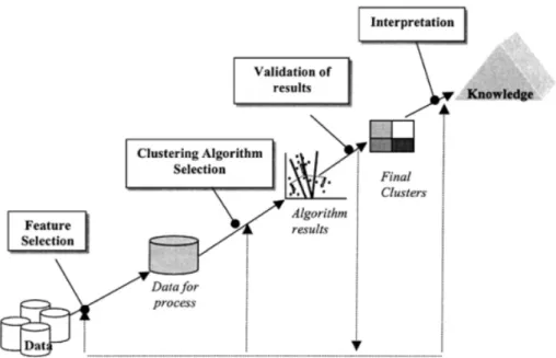
Figure 2 provides different steps of clustering and how clustering can be used for knowledge discovery from a data.
Figure 2 Different Steps in Cluster Analysis (Halkidi et al., 2001)
The basic steps that must be followed to perform cluster analysis are as follows:
1. Feature Selection
Features must be selected properly in order to encode as much information as possible concerning the task of interest. The major goal is minimum information redundancy among the features. As in supervised classification,
preprocessing of features may be necessary prior to their utilization in subsequent stages.
2. Proximity Measure
Proximity measure quantifies how “similar” or “dissimilar” two features are. It ensures that all selected features contribute equally to the computation of the proximity measure and there are no features dominating other features. Thus, selection of proximity measure is one important step in cluster analysis. This research focuses on evaluation of different proximity measures.
3. Clustering Criterion
Clustering criterion depends on the interpretation of the expert as “sensible” based on the type of clusters that are expected to underlie the dataset. The clustering criterion may be expressed as cost function or some type of rule depending on the dataset.
4. Clustering Algorithms
Here, a specific algorithm is selected that reveals the clustering structure of data set based on previously selected proximity measure and clustering criterion.
5. Validation of Results
The clustering algorithm provides the result of dataset as clusters, which needs to be verified using appropriate tests.
6. Interpretation of the Results
The resulting clusters must integrate the results of clustering with other experimental evidence and analysis in order to draw right conclusions. In most of the case, expert in application field is required to integrate the result.
Further, in some cases, Clustering Tendency should be involved which
includes various test that indicate whether or not the available data possess a clustering structure. This step is particularly important in case of completely random data where trying to find a cluster would be meaningless. The choice of features, proximity measures, clustering criteria and clustering algorithm is
important as they may lead to totally different clustering results (Theodoridis &
2.3 Assumptions in Cluster Analysis
Cluster Analysis is a method for quantifying the structural characteristics of a set of observations and has strong mathematical properties but does not have strong statistical foundation. Thus, there are certain assumptions to be made with respect to variables in the cluster variate.
One of the assumptions is representativeness of the sample. Usually, a sample case is obtained for clustering rather than the whole census data. Thus, it is assumed that the given sample of observation is the true representation of the population and the results are general to the population of interest.
Another assumption in cluster analysis is the impact of multicollinearity. Multicollinearity is the statistical phenomena where two or more variables are strongly correlated. In case of cluster analysis, the effect of multicollinearity is the form of implicit weighing and acts as a weighting process, which is not apparent to the observer but affecting the analysis. For example, when there are many variables in a dataset, and multicollinearity is examined with two sets of variables where one dataset has more variables than other. The effect on similarity measure would be large with dataset containing more variables. This is due to fact that each variable is weighted equally in cluster analysis. Thus, it is suggested to examine the variables used in cluster analysis for substantial multicollinearity and if present, either the number of variables is reduced to equal numbers in each set or one of distance measures such as
Mahalanobis distance that compensates for the correlation is used (Hair et al.,
2006).
2.4 Clusters analysis as measure of similarity
Similarity represents the degree of correspondence among objects across all
of the characteristics used in the analysis (Hair et al., 2006). The concept of
similarity is fundamental to cluster analysis and inter-object similarity is an empirical measure of correspondence, or resemblance between objects to be clustered (Hair et al., 2006).
Similarity provides the concept of proximity and presents how ‘close’ the observations are to each other or how ‘far’ are the observations. Similarity measures are most commonly used for the dataset with categorical variables.
The measures are generally scaled to be in the interval [0, 1], although occasionally they are expressed as percentages in the range 0–100%. Two individuals i and j have a similarity coefficient 𝑠!" of 1 if both have identical values for all variables. A similarity value of 0 indicates that the two
individuals differ maximally for all variables. (Everitt, 2011)
The input for a clustering method is a set of data vectors, where each data vector is a multidimensional set of data elements. The data vectors are compared for similarity and similar vectors are combined into clusters. Similarity in clustering is measured using a function, which takes two data vectors as input and returns a similarity value for them (Nikander, 2012). Similarity measure could be applied to identify the outliers in dataset, which could be observations with large distance from all other observations, or
appear in cluster as single member or a small cluster (Hair et al., 2006).
There are two ways of obtaining measures of similarity. First method is to directly obtain the similarity about the objects like by market survey or food testing experiment. Alternatively, similarity can be obtained indirectly from vectors of measurements or characteristics describing each object. However, in second case, it is necessary to define the idea of ‘similar’ in order to
calculate formal similarity measure. (Hand et al., 2001)
For measurement of similarity, three measures could be used namely, correlational measure, distance measure and association measure. Correlation measure uses correlation coefficient between the variables where higher correlation indicates similarity and lower correlation indicates lack of similarity. Association measure is used to compare objects whose
characteristics are measured only in nonmetric term. (Hair et al., 2006)
In this research, distance measure used to measure the similarity and is described in section 2.5.
2.5 Distance measures
Distance is the most common similarity measure used in case of cluster analysis. It is not entirely clear how a ‘cluster’ is recognized when displayed in the plane, but one feature of the recognition process would appear to involve the assessment of relative distances between points. The distance measures represent similarity as the proximity of observations to one another across the
variables in cluster variate. Distance measures are actually a measure of
dissimilarity for continuous variables (Everitt, 2011), where a larger value
denotes less similarity and is converted into a similarity measure by using an inverse relationship. The distance measure best represents the concept of proximity as it focuses on the magnitude of the values and portrays similar cases of the objects that are close together. As the characteristics measured by metric variables are used, distance measure is the best method to assess similarity in clusters. (Hair et al., 2006)
The different distance measures used in this research are explained in section 2.6 and 2.7.
2.6 Minkowski distance
Minkowski distance is the generalized form of different distance measures like Euclidean distance, Manhattan distance, Chebyshev distance and Hamming
distance. Minkowski distance of order P is defined as:
𝑑 𝑔!,𝑔! = |𝑔!(𝑥)− 𝑔!(𝑥)|! ! 𝑑𝑥 ! ! , 𝑝≥ 1
Where, g1(x) and g2(x) are functions of x and Y is the range of the integration.
If Y is an index set, Y= 1,2,….,𝑛 and g1(x) and g2(x) are real then, above equation can be written as:
𝑑 𝑔!,𝑔! = |𝑔!! −𝑔 !!|! ! !!! ! !
Which is the distance between two points 𝑔!!,𝑔
!!,…..,𝑔!! and 𝑔!!,𝑔
!!,…..,𝑔!! in 𝑅!. Alternatively, if X=[a, b] and g1(x) and g2(x) are 𝐿!
integrable which corresponds to: !|𝑔! 𝑥 |!
! |𝑑𝑥< ∞ and, |𝑔! 𝑥 |! ! ! |𝑑𝑥 < ∞, then 𝑑 𝑔!,𝑔! = !|𝑔!(𝑥)− 𝑔!(𝑥)|! ! 𝑑𝑥 ! !
Figure 3 Different forms of Minkowski distance
Minkowski distance is often used when variables are measured in ratio scales with absolute zero value. The Minkowski distance reduces to the rectilinear
distance, Euclidean distance and Chebyshev distance when the order p
equals to 1, 2 and ∞, respectively (Figure 3). The Minkowski distance is a
general formula where p=1 results in Manhattan distance, p=2 results in
Euclidean distance and 𝑝=∞ results in Chebyshev distance (Zhai et al.,
2014). The different forms of Minkowski distance between two points is represented in figure 3 and explained in this section.
The value of ‘p’ in Minkowski distance has its effect on type of clusters a distance measure produces. Figure 4 shows unit circles with various values of
‘p’ and corresponding shape of clusters produced as a result of ‘p’.
For 𝑝= 2, assumes circular cluster shapes, 𝑝= 1 assumes cluster in shape of square in two dimensions or diamond like in three or more dimensions and
𝑝= ∞ assumes clusters in the form of a box with sides parallel to the axes.
Also, 𝑝= ∞ and 𝑝= 1 could be particularly useful in cases where the data
structures have shapes with sharp edges. (Groenen & Jajuga, 2001). For
practical application, it is intuitive to use 𝑝=1, 𝑝 =2, or 𝑝= ∞ for Minkowski
distance (Zhai et al., 2014). Thus, these three different variations of Minkowski
distance are used as three different distance measures in this research.
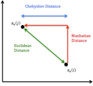
For a dataset with n data objects with p real valued measurements on each
object, the vector of observations for the ith object is denoted by 𝑥 𝑖 =
𝑥! 𝑖 ,𝑥! 𝑖 ,…,𝑥! 𝑖 , 1≤𝑖 ≤𝑛 , where the value of the kth variable for the ith
object is 𝑥!(𝑖). The different distance measures are defined below.
2.6.1 Euclidean Distance
This is the most commonly used distance between two points. It is simply the geometric distance in the multidimensional space and is extension to Pythagoras theorem.
Then the Euclidean distance between ith and jth object is defined as:
𝑑 𝑖,𝑗 = (𝑥! 𝑖 −𝑥! 𝑗 )! !
!!!
! !
In simpler terms, Euclidean distance is the shortest distance between two given points as represented in figure 5.
Euclidean distance can be interpreted as a physical distance between two p -dimensional points in Euclidean space. The Euclidean distance between two
vectors takes its minimum value 𝑑! =0 when the vectors coincide.
(Theodoridis & Koutroumbas , 2003)
This measure assumes some degree of commensurability between different variables. Thus, it would be effective if each variable were measured using same unit. Since the dataset often has non-commensurate variables, the arbitrariness of choice of unit must be overcome. A common strategy is to standardize the data by dividing each of the variables by its sample standard deviation so they are all regarded as equally important. Alternatively, data could be standardized by taking into account the covariance between the variables. The Euclidean distance is additive in the sense that the variables
contribute independently to the measure of distance. (Hand et al., 2001)
2.6.2 Squared Euclidean Distance
Squared Euclidean distance is the sum of the squared differences without taking the square root. The squared Euclidean distance has the advantage of not having to take the square root, which speeds the computations markedly
(Hair et al., 2006). The squared Euclidean distance is used more often than Euclidean distance to place progressively greater weight on objects that are
further apart (Sage Publications, 2008). The values are calculated for each
object pair by summing the squared difference between the observations.
The Squared Euclidean distance between ith and jth object is defined as:
𝑑 𝑖,𝑗 = (𝑥! 𝑖 −𝑥! 𝑗 )! !
!!!
Square Euclidean distance is not a metric, as it does not satisfy the triangle inequality, however it is used in problems in which only distance have to be compared. Generally, Squared Euclidean distance and Euclidean distance is
computed from raw data and not from standardized data (Sage Publications,
2008). It has wide spread use among researchers in the social and behavioral
2.6.3 Manhattan Distance
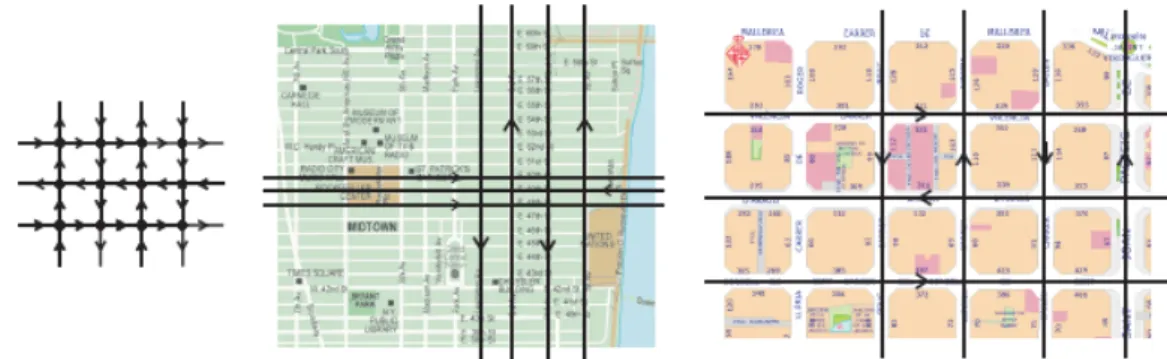
Manhattan distance is based on Manhattan network which is a unidirectional regular mesh structure resembling locally the topology of the avenues and
streets of Manhattan (Dalfo et al., 2007). Manhattan distance can be defined
as distance between two points in Euclidean space with fixed Cartesian coordinate system. It is the sum of the lengths of the projections of the
segment between the points into the coordinate axes (Wikia, 2013).
Figure 6 The local pattern of a Manhattan network and real life examples of orthogonal streets of Manhattan and Barcelona (Dalfo et al., 2007)
Manhattan distance is the distance between two points measured along axes at right angles and is often referred as city block distance as it measures distances travelled in street configuration. The Manhattan distance between
ith and jth object is defined as:
𝑑 𝑖,𝑗 = |𝑥! 𝑖 −𝑥! 𝑗 !
!!!
|
In simpler terms, Manhattan distance is the sum of horizontal and vertical components between the given points in a plane.
Figure 7 Manhattan distance (red); equivalent Manhattan distance (yellow and blue) and Euclidean distance (green) between two points (Wiktionary, 2013)
In figure above, the path represented by the red, blue or yellow lines, which is to be followed to reach from the point of origin to destination point in a Manhattan network is the Manhattan distance. It is also known as rectilinear
distance, L1 distance or l1 norm, city block distance or Manhattan length.
Manhattan distance depends on the choice of the rotation of the coordinate system, but does not depend on the translation of the coordinate system or its reflection with respect to a coordinate axis (Wikia, 2013). It uses the sum of absolute differences of the variables and is simple to calculate but may lead
to invalid clusters if the clustering variables are highly correlated (Hair et al.,
2006).
2.6.4 Chebyshev Distance
The Chebyshev distance is one extreme case of Minkowski distance where
𝑝= ∞ is used that makes the distance equal to the single largest attribute
value difference (Cichosz, 2015). The Chebyshev distance is also known as
maximum value distance and calculates absolute magnitude between values of two objects. It is appropriate in cases when two objects are to be defined
as “different” if they are different in any one dimension (University of Texas,
2000).
Chebyshev distance is a metric defined on a vector space where distance between two vectors is the greatest of their difference along any coordinate dimension.
Figure 8 Chebyshev distance between two points
The Chebyshev distance (Figure 8) represents the distance along the largest dimension between two points. The Chebyshev distance are piecewise linear and in process of clustering, it ensures that the next considered points are
potentially located at the border of neighborhood of point in one dimension, and these point usually discover an unexplored area of the search space.
(Dillmann et al., 2010)
Then the Chebyshev distance between ith and jth object is defined as:
𝑑 𝑖,𝑗 = lim !→! (𝑥! 𝑖 −𝑥! 𝑗 ) ! ! !!! ! ! = 𝑚𝑎𝑥 𝑥! 𝑖 −𝑥! 𝑗
The Chebyshev distance is also known as Chess distance and is the distance between squares, in terms of move necessary for a King to go from one
square to another. The circle of radius r, in Chebyshev metric is a square with
side of length 2r parallel Euclidean distance (Agarawal & Sahoo, 2008).
Figure 9 Unit Circle representation of Chebyshev distance
Chebyshev distance is often used in cases where the execution speed is so critical that the time involved in calculating the Euclidean distance is unacceptable. The contour lines of equal Chebyshev distance from a point
are squares in two dimensions (Webb, 1999). It reduces the unit circle to a
square with sharp edges (figure 9) hence, is useful to determine clusters with sharp edges. The major advantage of the Chebyshev distance is that it requires less time to decide the distances between the datasets. However, with the Chebyshev distance, one single feature is allowed to represent a dataset. This one single largest feature might not offer enough description of the dataset to lead to accurate neighborhood selection and final predictions
(Filipe & Cordeiro, 2011). Thus, there might be case where Chebyshev distance could favor one dataset over another when different dataset are combined for clustering purpose.
2.7 Mahalanobis Distance
Mahalanobis distance is a generalized distance that accounts for the correlation among variables in a way that weights each variable equally. It
also relies on standardized variables (Hair et al., 2006). A dataset could be
standardized using covariance between the variables. The covariance
between variable X and Y is calculated as:
𝐶𝑜𝑣 𝑋,𝑌 = 1
𝑛 (𝑥 𝑖 −𝑥) (
!
!!!
𝑦 𝑖 −𝑦)
Where, 𝑥 is mean of X values and 𝑦 is the mean of Y values.
When the covariance matrix is incorporated in definition of distance,
Mahalanobis distance between two p-dimensional measurements 𝑥 𝑖 and
𝑥 𝑗 is obtained which is defined as:
𝑑!" 𝑖,𝑗 = 𝑥 𝑖 −𝑥 𝑗 ! !! 𝑥 𝑖 −𝑥 𝑗 ! !
Where, T represents the transpose, is the p x p sample covariance matrix,
and !! standardizes the data relative to . (Hand et al., 2001)
In simpler terms, Mahalanobis distance is distance between a point and a
distribution of data (Mahalanobis, 1936). It measures how many standard
deviations away a point is from the mean of distribution. As represented in Figure 10 (plot b) below, when the point is in the mean of distribution of data, Mahalanobis distance is zero and as the point moves away from the mean of distribution of data, Mahalanobis distance increases.
Figure 10 Comparison between Euclidean distance and Mahalanobis distance (Maesschalck et al., 2000)
Since, it is intuitive to understand Euclidean distance, figure 10 provides the comparison between Euclidean distance and Mahalanobis distance. In figure,
part (a) is the plot of the simulated data for two variables x1 and x2 together
with the circles representing equal Euclidean distance towards the center point. Part (b) is the plot of the simulated data for two variables x1 and x2
together with the ellipses representing equal Mahalanobis distance towards the center point. When Euclidean distance is used, the set of point equidistant from a given location is a sphere whereas; the Mahalanobis distance stretches the sphere to correct for the respective scales of the different variables and to account for the correctional among the variables providing ellipsoidal shape (Manly, 1986). As Mahalanobis distance takes covariance as well as direction of covariance of data into account, distance varies according to spread of the data. (Maesschalck et al., 2000).
The Mahalanobis distance increases with increasing distances between the two group centers and with decreasing within-group variation. Mahalanobis distance takes account of shape of the clusters by employing within-group
correlation. (Everitt, 2011)
2.8 Selecting the best distance measure
As there are different distance measures for analyzing similarity, the ideal question rises about the selection of the best measures. However, selection of best distance measure is not straightforward and rather depends on different factors of the observed dataset. Everitt (2011) mentioned the influence of nature of data on choice of proximity measure. Also, the choice of measure should depend on scale of data as they provide different cluster solutions. For continuous data, distance or correlation-type dissimilarity measures should be used. Further, the clustering method used might have certain implications for the choice of parameters.
Hair (2006) has purposed few issues to be taken into consideration while selecting the best distance measure. As mentioned earlier by Everitt (2011) change in scale of variables may lead to different cluster solutions and comparing the result with theoretical or known pattern provides better solution to given problem. When the variables are correlated, Mahalanobis distance
measure is likely to be most appropriate as it adjusts for correlation and
weights all variable equally (Hair et al., 2006).
2.9 Clustering Methods
There are different methods in determining and describing a cluster. However, different methods or even a same method with different parameter configurations can produce different clustering result. Clustering methods differ in many ways including definition of distance between data items, definition of ‘cluster’, the strategy to group or divide data items into clusters and, the data type that can be analyzed (numerical, categorical) and
application-specific context and constrains (Miller & Han, 2001).
In general, the clustering method can be categorized into following five categories
1. Partitioning Methods 2. Hierarchical Methods 3. Density Based Methods 4. Grid Based Methods 5. Fuzzy Clustering
2.9.1 Partitioning Methods
For the dataset of n objects, partitioning methods creates the K number of
partition for the given dataset where each partition corresponds to a cluster. In this method, each partition should contain at least one object and each object should only belong to one partition. The clusters are formed to optimize an objective-partitioning criterion, such as a dissimilarity function based on distance. It creates an initial partitioning and uses iterative relocation technique that attempts to improve the partitioning by moving objects from
one group to another. (Miller & Han, 2001)
There are different partitioning methods, two of which are described below.
K-means
K-means is a typical partitioning method where the given dataset is
partitioned into K number of clusters. In k-means method, cluster similarity is
measured with respect to the mean value of the objects in a cluster, which can be viewed as the cluster’s centroid or center of gravity.
K-means algorithm is used to determine the clusters. In the algorithm, it
randomly selects K of the objects, each of which initially represents a cluster
center. For each remaining objects, an object is assigned to the cluster to which it is the most similar based on the distance between the object and the cluster mean. It then computes the new mean for each cluster. The algorithm iterates until the center of the clusters does not change, which corresponds to convergence of criterion function. The main aim of K-means clustering is the optimization of the objective function based on input parameters. The
algorithm attempts to determine k partitions that minimize the objective
function used, which is defined by square-error criterion.
The square-error criterion is used as stoppage criteria of the algorithm, which is defined as,
𝐸 = 𝑝−𝑚! ! !∈!!
!
!!!
Where, E is the sum of square-error for all the objects in the dataset; P is the
point representing a given object and 𝑚! is the mean of cluster 𝐶!.
Here, for each object in each cluster, the distance from the object to its cluster center is calculated, and the distances are summed up. This criterion tries to
make the resulting K clusters as compact and as separate as possible. The
criterion function attempts to minimize the distance of each point from the center of the cluster to which the point belongs.
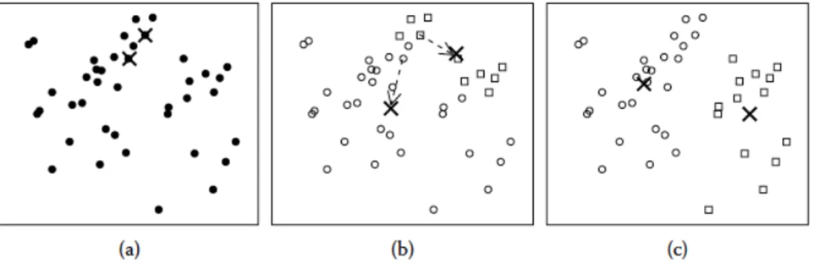
Figure 11 K-Means clustering algorithm steps (Miller & Han, 2001)
Figure 11 represents clustering process for the k-means algorithm with two clusters. In figure 11 (part a), for the dataset, two random cluster centers are selected (marked with ‘x’). Further, when the points are assigned to a cluster based on its distance to cluster centers, the cluster centers starts to move
from its initial location as represented in part b. Finally, when there are no more points remaining to assign to the cluster, the center of cluster does not change and final solution, containing two distinct clusters and two cluster centers are obtained as represented in part c. The pseudo code for K-means algorithm is presented in Appendix 1.
In K-means, random initialization of centroids is used, thus, different runs of K-means can produce different clusters. Selecting the proper initial centroids is the key step of the basic K-means method. Since, the initial centroids are selected randomly, it might not be possible to replicate exact cluster in different runs of algorithm. Thus, to solve the problem, one effective approach is to take a sample of points and cluster them using a hierarchical clustering technique. From hierarchical clustering, K clusters are extracted and centroids of those clusters are used as initial centroids for K-means clustering. Another approach is, by selecting first point at random or by taking the centroid of all points. Then for each successive initial centroid, the point that is farthest from any of the initial centroid is selected. By this approach, the initial centroids are guaranteed not only to be randomly selected but also well separated. But this approach can select outliers, rather than points in cluster and also it is expensive to compute the farthest point from the current set of initial centroids. Thus to overcome these problems, this approach is applied to sample of the points as outliers are rare, they tend not to show up
in a random sample. (Tan et al., 2006)
The algorithm works well when the clusters are compact clouds that are well separated from one another. The method is relatively scalable and efficient in processing large dataset because the computational complexity of the
algorithm is O(nkt), where n is the total number of objects, k is number of
clusters, and t is the number of iterations. The method terminates at a local
optimum. The output of algorithm produces clusters and cluster center is represented by the mean value of the objects in the cluster.
Although the algorithm partitions the given dataset into desired number of clusters, specifying the number of clusters in advance can be a disadvantage. Further, the method is not suitable for discovering clusters with non-convex shapes of clusters of different size and is sensitive to noise and outlier data