SELF-SUPERVISED LEARNING OF SPATIOTEMPORAL FEATURES FROM VIDEO COLORIZATION
BY
ZUBIN PAHUJA
THESIS
Submitted in partial fulfillment of the requirements for the degree of Master of Science in Computer Science
in the Graduate College of the
University of Illinois at Urbana-Champaign, 2019
Urbana, Illinois
Adviser:
ABSTRACT
We pose video colorization as a self-supervised learning problem for visual tracking. We use large amounts of freely available unlabeled video from YouTube to learn colorization without explicit supervision. However, instead of predicting the color directly from the gray-scale frame, we constrain the model to solve this task by learning to copy colors from a reference frame. By equipping the model with a pointing mechanism into a reference frame, we learn an explicit spatiotemporal feature representation that can be used as a generic tracker for new tracking tasks without additional training or fine-tuning.
Our self-supervised model can propagate any annotation from the first frame as a reference to the rest of the video. Experimental results suggest that the learned feature representations can be effectively transferred to video tracking and object segmentation tasks. We perform extensive quantitative and qualitative evaluations on the DAVIS-2017 video object segmentation dataset and demonstrate significant improvements over the baseline. Although the model is trained without any ground-truth labels, our method learns to track well enough to outperform the latest methods based on optical flow.
Since annotating videos is expensive and tracking has many applications in robotics and graphics, we believe learning to track with self-supervision can have a large impact. More broadly, we show that the features learned from a task for which cheap training data is readily available can be used to learn a task which would otherwise require an expensive, large-scale dataset with minimal supervision. Thus, we hope our results encourage a broader exploration in the promising field of self-supervised learning.
To my Godmother, for instilling faith in me. To my parents, for placing their faith in me.
ACKNOWLEDGMENTS
First and foremost, I would like to express my sincere gratitude to my research advisor, Dr. David Forsyth for his inspirational guidance that left me in awe of his intellect and humility and filled me with joy and enthusiasm for research every time I sought his advice. I feel privileged and grateful for this incredibly kind opportunity of a lifetime.
I am thankful to my friends and family for seeing me through thick and thin. Special thanks to Nilesh sir and Swati ma’am, Bakul uncle and Nita aunty without whom none of this would have ever been possible, and who are no less to me than my parents.
I would also like to take this opportunity to thank the Computer Vision research group members for inspiring and informing me, the Association for Computing Machinery (ACM) chapter at University of Illinois, Urbana-Champaign (UIUC) for fostering an exuberant learning community, the Department of Computer Science, especially my undergraduate research advisor, Dr. Kevin Chang and my graduate academic advisor, Viveka Kudaligama for their continued support.
TABLE OF CONTENTS
LIST OF TABLES . . . vi
LIST OF FIGURES . . . vii
CHAPTER 1 INTRODUCTION . . . 1
CHAPTER 2 RELATED WORK . . . 3
2.1 Self-Supervised Learning . . . 3
2.2 Colorization . . . 3
2.3 Video Object Segmentation . . . 4
2.4 Unsupervised Tracking . . . 4
2.5 Attention Mechanism . . . 5
CHAPTER 3 SELF-SUPERVISED COLORIZATION . . . 6
3.1 Hypothesis . . . 6
3.2 Model . . . 7
3.3 Learning . . . 8
3.4 Inference . . . 9
3.5 Implementation . . . 9
CHAPTER 4 UNSUPERVISED TRACKING . . . 13
4.1 Task . . . 13
4.2 Baseline . . . 14
4.3 Tracking from Colorization . . . 15
4.4 Denoising with MRFs . . . 15
4.5 Segmentation with Graph Cuts . . . 19
4.6 Results and Analysis . . . 21
CHAPTER 5 CONCLUSION . . . 24
LIST OF TABLES
3.1 Network Architecture: The table outlines the architecture of our 3D Convolutional network. Each convolution is followed by batch normalization and a rectified linear unit (ReLU), except for the last 1x1 convolution layer which produces the feature embeddings. The kernel
size is specified in the Time x Width x Height notation. . . 11 4.1 DAVIS 2016: Single-object video segmentation. . . 21 4.2 DAVIS 2017: Multi-object video segmentation. . . 21
LIST OF FIGURES
1.1 Tracking from Colorization: The figure illustrates the problem setup wherein the model learns to predict colors for a gray-scale frame by pointing to the corresponding pixel in the reference frame and copying its color. Thereby, a pointing mechanism is implicitly learned, which can be
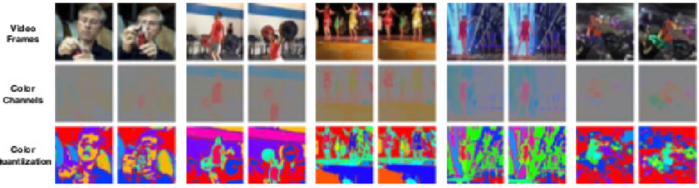
used as a tracker for downstream tasks. . . 2 3.1 Temporal Coherence of Color: Objects can be distinguished and
matched across two video frames that are seconds apart from their colors alone. This observation is generally true even if objects are arbitrarily displaced, but it fails under illumination changes as shown in the last column. The first row shows original frames, and the second row shows ‘ab’ color channels from Lab space. The third row quantizes colors into discrete bins and perturbs the colors to make the effect more
pronounced. Image courtesy: Vondrick et al. [1] . . . 6 3.2 Model Overview: The model uses a 3D CNN to compute feature
embeddings for every pixel in the gray-scale reference and target frames. For each pixel in target frame, the model points to the pixel in reference frame with the most similar embedding as measured by vector dot product (solid yellow arrow). It copies the color channels at that location in the RGB reference frame back to the predicted colors frame (dashed yellow arrow). At inference time, this pointing mechanism learned from colorization as a proxy task, is used for tracking. Although the illustrated pointer points to a single pixel, the actual pointer is “soft” in
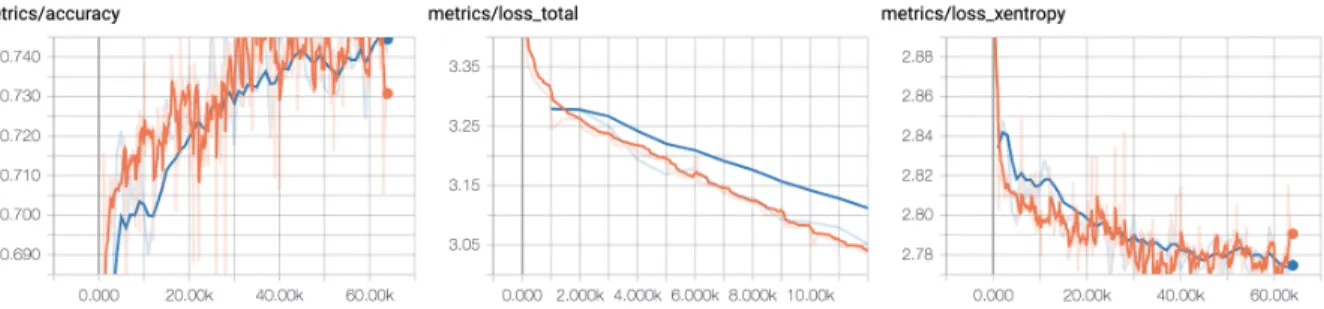
the sense that it uses softmax-similarity to copy a weighted color distribution. 7 3.3 Training and Validation History: Graphs of accuracy and loss vs epochs. 11 3.4 Video Colorization: Given a reference frame, our model learns to copy
colors over many challenging transformations such as fast motion. . . 12 4.1 Davis 2017: A multi-instance video object segmentation dataset. . . 13 4.2 Discrete MRF for Image Denoising: The shaded nodes represent the
observed pixel valuesXi, and the open nodes represent the unknown, true pixel values Hi. Each Xi is connected to the corresponding Hi, and each
Hi is connected to its neighbors Hj. . . 16 4.3 Examples of GrabCut: The user drags a rectangle loosely around an
object. The object is then extracted automatically. Image Courtesy:
4.4 Graphical Model for GrabCut: Each node in the graph represents pixels in the image. In addition, every pixel node in the graph is connected to the Source and Sink nodes, which represent the foreground and the background of the image respectively. A Min-cut/Max-Flow algorithm is
used to extract the foreground from the background. . . 20 4.5 Qualitative Evaluation: Figure shows ground truth annotation, our
self-supervised tracker, and then results refined using MFI and GrabCut
CHAPTER 1: INTRODUCTION
Visual tracking, or the process of locating one or more moving object(s) in a video over time, remains an active area of research in computer vision. Use cases include tracking of pedestrians by self-driving vehicles, or shoppers at an Amazon Go store as they just walk out with the products they intend to purchase. It has several other applications in robotics, human-computer interaction, security and surveillance, augmented reality (AR), medical imaging, video editing, video summarization, and video compression. Hence, tracking is integral to video analysis, and a good tracker must perform well in a large number of videos involving illumination changes, occlusion, camera motion, low contrast, and specularities.
However, the best performing deep learning-based techniques rely on copious amounts of labeled data, which requires extensive human effort to annotate every frame of the video. This approach is very expensive and prohibitive. We pursue an alternative approach that learns to track without human supervision by instead leveraging large amounts of raw, unlabeled video data.
The theme of our research is to learn feature embeddings from a task for which cheap training data is available in abundance. Then use these features to learn a task which would otherwise require an expensive large scale dataset. To this end, we take a self-supervised learning approach that uses video colorization as a supervisory signal for learning to track. Consecutive video frames are manipulated to generate pairs of gray-scale input and RGB labels, which yields ample training data to learn colorization at no cost.
The key intuition here is that colors in consecutive frames are temporally coherent. Hence, the object of interest in one frame will have a similar color in the subsequent frames. So instead of predicting the colors directly from the gray-scale frame, we take a roundabout approach by constraining the model to copy colors from a reference frame. This requires the model to learn to point to the region corresponding to the object in the reference frame. This pointer acts as a tracker in time.
After training on unlabeled videos collected from the web [3], the feature representation learned from video colorization can then be used for downstream tracking tasks without additional training or fine-tuning. We evaluate the performance of the tracker on the task of unsupervised video object segmentation against the 2017 DAVIS Challenge dataset and benchmark [4]. The model is set up to track segmented regions using the first frame of the video as reference. Experimental results demonstrate our tracker performs much better than optical flow, especially for the types of motion characterized by fast motion, occlusions, and dynamic backgrounds.
Figure 1.1: Tracking from Colorization: The figure illustrates the problem setup wherein the model learns to predict colors for a gray-scale frame by pointing to the corresponding pixel in the reference frame and copying its color. Thereby, a pointing mechanism is implicitly learned, which can be used as a tracker for downstream tasks.
However, the tracker has certain limitations, since the model is explicitly trained for video colorization. Low contrast video frames and camouflaged instances do not require the model to produce very accurate mappings to colorize successfully. These instances are also naturally hard to segment since their edges are not distinctly visible. Other known, stubborn problems such as objects with fine-structures remain difficult. But the most pressing problems arise when parts of other objects in the scene have a very similar structure and intensity to the tracked object. This leads to discontinuities in the predicted segment and mispredictions of other object parts as the target segment, which appear as blobs.
To address these limitations, mean-field variational inference (MFI) is employed at inference time to denoise and smoothen the segmentation mask. This removes any holes in the predicted segment or redundant blobs that the model may have over-eagerly predicted as a target segment. An artifact of this smoothening though is the expansion and blurring of segmentation boundary. To counteract this undesirable side-effect, we iteratively extract the precise object segmentation using automatic “GrabCut” [2].
Our self-supervised tracker performs significantly better than optical flow (FlowNet 2) without any labeled data during training. Therefore, these results underscore the promise of self-supervised learning and encourage further investigations in this emerging field of study.
CHAPTER 2: RELATED WORK
2.1 SELF-SUPERVISED LEARNING
Labeling millions of images for individual tasks in computer vision is expensive. An alternative training approach is self-supervised learning: supervised learning that does not require manually annotated data since labels are “manufactured” from unlabeled data.
A growing body of work capitalizes on large amounts of unlabeled video to train visual models by leveraging the natural context in images [1, 5–20]. The idea is to design auxiliary tasks to learn visual representations, which can then be used as a feature space for downstream tasks. Most of these auxiliary tasks learn specific kinds of invariance, such as spatial context [5], sounds associated with video frames [6, 7], inpainting [8], and color.
Other approaches include using robots that interact with the environment to learn visual features [21–23]. A related but different line of work explores how to learn geometric properties or cycle consistencies with self-supervision, for example for motion capture and visual correspondence [24–28], or audio source localization and separation [7].
The performance of these self-supervised models has come tantalizingly close to their supervised counterparts for several tasks, namely visual understanding [10], activity recognition [11], video generation [11], object classification and detection [12–14] among several others [15–19]. Furthermore, convolutional neural networks (CNN) trained with pre-trained feature representations from self-supervised models perform significantly better than randomly initialized networks and achieve state-of-the-art performance among algorithms which use only training set annotations [9, 10].
2.2 COLORIZATION
The task of colorization for gray-scale images and video has drawn significant attention in the vision community [29–38]. Apart from the principal task, it has also been leveraged as a proxy task to learn feature representations without explicit supervision [1, 10, 15].
In the context of video colorization, approaches that explicitly incorporate optical flow or learn to propagate color have been explored. We pursue a similar yet different direction by taking an indirect approach to video colorization in order to learn to track. We capitalize on the temporal coherence of color rather than enforcing it within the model.
2.3 VIDEO OBJECT SEGMENTATION
Performance on video object segmentation task serves as an important yardstick for visual tracking. Specifically, we evaluate our tracker on DAVIS 2017 Challenge dataset [4], which is a widely adopted benchmark in the community. The task of the challenge is to densely label one or more objects in every frame of the video for the semi-supervised scenario, i.e. the segmentation mask of the first frame is given, and no human interaction or refinement is allowed. Region Jaccard and Boundary F-measure are used for performance measurement.
A taxonomy of approaches to video object segmentation classifies them into methods that use the object of interest as the starting point of inference [39–42], and those that do not [43–46]. It is a challenging task, and the models [47, 48] that achieve the best results use large scale labeled datasets such as ImageNet [49], MS-COCO [50] or DAVIS [4] for training. Instead of competing with these supervised methods, we pursue an entirely different direction for learning to track from unlabeled videos collected from YouTube [3].
2.4 UNSUPERVISED TRACKING
Unsupervised learning techniques for video tracking have traditionally employed non-parametric graphical models. Faktor et al. [51] cast video segmentation as an iterative consensus voting scheme on the graph of re-occurring regions. M¨arki et al. [52] perform a graph cut over a spatiotemporal bilateral grid.
On the other hand, Khoreva et al. [53] propose an alternative training strategy for ConvNets, which achieves state-of-the-art results while using 20x-1000x less annotated data. It generates in-domain training data using the provided annotation on the first frame of each video to synthesize (“lucid dream”) plausible future video frames. However, their approach requires training on the testing frames, and thus it is quite slow for practical use. Unlike the aforementioned approaches, our self-supervised neural network does not hand engineer objective functions. Consequently, our model serves as a generic tracking method applicable to many video analysis tasks, not only video segmentation. The trained model can track objects, colorize video, and transfer any other annotation from the first frame to the rest of the video, without any fine-tuning or re-training. Our approach is fairly practical. It is fast, can track multiple objects and does not require training on the testing frames.
2.5 ATTENTION MECHANISM
Attention mechanism was created to help memorize long source sentences in neural machine translation [54]. Rather than building a single context vector from the encoder's last hidden state, the proposed attention model by Bahdanau et al. [54] learns to soft-search for parts of a source sentence that are relevant to predicting a target word. Vinyals et al. developed upon this model and introduced an architecture called Pointer Net [55], which uses the attention mechanism of [54] as a pointer to select a member of the input sequence as the output.
These developments inspired the genesis of visual attention models that were designed to “focus” their “awareness” to the relevant region of the image by selective cropping. Borrowing insights from how a human eye works, Mnih et al. proposed Recurrent Attention Models (RAM) [56] that “take a glance” at the image around a given location and sequentially point to the next location to “glimpse”. Additionally, they are able to track simple objects without explicit training.
Subsequently, Jaderberg et al. introduced Spatial Transformer Networks [57] that spatially transform (and thus attend) feature maps, which results in models that learn invariance to translation, scale, and rotation. In stark contrast with RAMs, Spatial Transformer modules are trained to predict affine transformations without supervision, learned purely with backpropagation without reinforcement learning, and are more flexible. Our model uses a pointing mechanism similar to [54–57]. However, our approach is unsupervised and we train the model to learn a “soft” pointer for use as a visual tracker. Our model points within a single training example rather than across training examples, uses a differentiable objective function and hence, does not require reinforcement learning.
We acknowledge the pioneering work by Vondrick et al. [1], which forms the basis of our research. We use their model as baseline, significantly improve both the Jaccard and boundary F-measure for DAVIS 2017 dataset, and conduct in-depth analysis of the results.
CHAPTER 3: SELF-SUPERVISED COLORIZATION
Figure 3.1: Temporal Coherence of Color: Objects can be distinguished and matched across two video frames that are seconds apart from their colors alone. This observation is generally true even if objects are arbitrarily displaced, but it fails under illumination changes as shown in the last column. The first row shows original frames, and the second row shows ‘ab’ color channels from Lab space. The third row quantizes colors into discrete bins and perturbs the colors to make the effect more pronounced. Image courtesy: Vondrick et al. [1]
The chapter describes our self-supervised model, which is designed to learn a tracker using colorization as a proxy task. Then, the network architecture and implementation are described in details, followed by results that validate our hypothesis.
3.1 HYPOTHESIS
Our approach leverages the assumption of temporal coherency of color in videos to “manufacture” labels from unlabeled data at a large scale. Obviously, this assumption does not always hold true. For example, colorful lights can turn on or off, and an object can go out of the scene or another unseen object can appear in the frame. However, unlabeled video on the web, of which there is no deficit, often has temporally stable color in practice. Hundreds of thousands of raw, unlabeled ten seconds video clips [3] are fed into the network during training to satisfy the appetite of our model. The network is used to learn feature representations that point a pixel in the target frame back to its corresponding pixel in the reference frame(s). As a result, a pointing mechanism is learned which can be used for unsupervised visual tracking, or to propagate any annotation from the first frame to the rest of the video in general.
Figure 3.2: Model Overview: The model uses a 3D CNN to compute feature embeddings for every pixel in the gray-scale reference and target frames. For each pixel in target frame, the model points to the pixel in reference frame with the most similar embedding as measured by vector dot product (solid yellow arrow). It copies the color channels at that location in the RGB reference frame back to the predicted colors frame (dashed yellow arrow). At inference time, this pointing mechanism learned from colorization as a proxy task, is used for tracking. Although the illustrated pointer points to a single pixel, the actual pointer is “soft” in the sense that it uses softmax-similarity to copy a weighted color distribution.
3.2 MODEL
The model uses a spatiotemporal 3D-CNN to estimate a low-dimensional embedding vector
f ∈ RD for every pixel location in an image. The embeddings are used to compute an all-pairs similarity matrixA between the reference frame and the target frame, where distances are measured by inner-product. For pixel i in the reference frame and pixelj in the target frame, the similarity matrix is given byAij =fiTfj.
The similarity matrix A can be used to identify the pixel location in the reference frame that is the closest in embedding space to pixelj in the target frame, given by arg max
i
(Aij). This yields a “hard” pointer as illustrated in Figure 3.2.
However, the model learns a “soft” pointer instead. Rather than pointing to a single pixel in the reference frame, the model predicts the weighted color distribution of the pixels in the reference frame. The weights are given by the columns of the similarity matrix A after it has been normalized using softmax function such that the columns sum to one:
Aij =
exp(fT i fj) P
The “soft” pointing mechanism can be interpreted as a mixture model of colors/labels, where the softmax similarity matrix A gives the mixing coefficients. To define this model formally, let ci ∈Rd be the true color for pixel i in the reference frame, and cj ∈Rd be the true color for pixel j in the target frame. The model predicts a color yj ∈ Rd for pixel j in the target frame as a linear combination of colors in the reference frame:
yj = X
i
Aijci (3.2)
Due to the softmax-similarity, the model only needs to point to one pixel in the reference frame in order to copy a color. Consequently, if there are two objects with the same color, the model does not constrain them to have the same embedding and hence, it is able to track multiple objects of the same color similar to attention mechanism [54–57].
3.3 LEARNING
The model is trained on the Kinetics human action recognition dataset [3] for the task of video colorization. The dataset comprises of approximately 650,000 high-quality video clips collected from YouTube, with each clip lasting around 10 seconds. However, the labels are irrelevant and swiftly discarded.
The learning objective is to find network parameters θ such that the predicted colors yj are close to the target colors cj. There exist multiple ways to colorize a video. Therefore, it is a multi-modal problem with several local optima. We take the standard approach of quantizing the color-space into discrete categories, and then optimizing the cross-entropy categorical loss function, L=−P
iyilog ˆyi across the training dataset: min
θ X
j
L(yj, cj) (3.3)
In our case, we quantize the color space into 32 color channels estimated by k-means clustering over 10,000 video clips from the Kinetics training data. The choice of these parameters achieves the best results on the DAVIS 2017 Challenge [4].
We use Adam optimizer [58] to optimize equation (3.3). Further details of the choice of hyper-parameters used for learning are provided in the Implementation section.
3.4 INFERENCE
Once trained, the 3D-CNN model outputs embeddings for every pixel in an image, which is used to compute a similarity matrix A for a pair of reference and target frames.
In order to colorize the target frame, the color channels in the reference frame are first quantized into k = 32 discrete bins. The quantization makes use of the cluster centers pre-computed using k-means. The cluster center closest to the color of the pixel is assigned as the quantized color value. The quantized color is then expressed as a one-hot vectorci ∈Rk. Now, we simply use the equation (3.2) to predict and propagate colors from the reference frame to the target frame. However, we make two small modifications during inference:
First, we use a recursive approach to propagate color. At each time step, the model predicts the colors for the current frame using a window of previousN = 3 frames as references. Only the first window consists of the ground truth RGB frames, and the remaining comprise of the model’s predictions. This trick helps reconcile with the problems caused by drift. Although the training video clips from Kinetics dataset are no longer than ten seconds, but this trick comes in handy when the model is used to colorize longer length videos and the objects get farther away from their original position in the reference frame.
Second, we adjust the temperatureτ of the softmax. Pre-softmax activationszare divided by a constant temperature τ before they are normalized, as defined below:
σ(z)i =
exp(zi/τ) P
jexp(zj/τ)
(3.4) The columns of the softmax similarity matrix, as defined in equation (3.1), give the weights for averaging colors/labels for pixels in the reference frame. The weights serve as a “soft” pointer, and the weighted average is returned as the model’s prediction. As the model propagates the distribution of colors, the results may become blurry with time if this pointer is not accurate. To compensate for this, the temperatureτ of the softmax is reduced during inference, so that the pointer makes more accurate predictions over time. We use τ = 0.5 for inference, but set τ = 1 to leave softmax as is for training. Equation (3.1) then becomes:
Aij = exp(fT i fj/τ) P kexp(fkTfj/τ) (3.5) 3.5 IMPLEMENTATION
We use a pre-trained ResNet-18 followed by a 5-layer 3D-CNN network to produce 64-dimensional feature embeddings per pixel. The embeddings are used to compute the all-pairs
similarity matrix between the reference frame and the target frame, which can be larger than the compute memory available. However, since color has low spatial frequency in images, we are able to operate at a low resolution that allows us to fit the matrix into available space. Hence, the model predicts a down-sampled feature map for both the reference and the target frame. We observe the best results with a 64 x 64 resolution color map before we run out of memory. Our implementation uses TensorFlow [59] and OpenCV [60].
3.5.1 Input
The network takes three reference frames and a target frame as its input. A window of three frames prior to the target frame is used as reference. All input frames are gray-scale and down-sampled to 256 x 256 resolution.
3.5.2 Data Preprocessing
We adhere to the standard practices for image processing. For gray-scale input images, the intensities are scaled in the range [-1,1].
For the colored reference frame(s), the RGB image is first converted into Lab color-space, and then the ’ab’ color channels are quantized into 32 discrete bins using k-means. The quantized color is represented as a one-hot vector, which is “hot” at the index corresponding to the nearest cluster center.
3.5.3 Network Architecture
The original ResNet-18 architecture [61] that has been pre-trained on ImageNet [62] is used as a backbone for our network. However, the ResNet architecture is slightly modified. The fully-connected layers used for classification and the last global average pooling layer are removed, and the output stride is modified such that the network outputs a 32 x 32 spatial map of 256 dimensions each.
Each input frame is propagated forward through the ResNet to extract feature representations of the dimensions 32 x 32 x 256. The pixel coordinates are encoded as a two-dimensional vector in the range [-1,1] and the vector is concatenated to the features from the ResNet in order to include global spatial information in the image representations.
Type Kernel Size Num Outputs Stride Padding Dilation Convolution 1 x 3 x 3 256 1 1 1 x 1 x 1 Convolution 3 x 1 x 1 256 1 1 1 x 1 x 1 Convolution 1 x 3 x 3 256 1 1 1 x 2 x 2 Convolution 3 x 1 x 1 256 1 1 1 x 1 x 1 Convolution 1 x 3 x 3 256 1 1 1 x 4 x 4 Convolution 3 x 1 x 1 256 1 1 1 x 1 x 1 Convolution 1 x 3 x 3 256 1 1 1 x 8 x 8 Convolution 3 x 1 x 1 256 1 1 1 x 1 x 1 Convolution 1 x 3 x 3 256 1 1 1 x 16 x 16 Convolution 3 x 1 x 1 256 1 1 1 x 1 x 1 Convolution 1 x 1 x 1 64 1 1 1 x 1 x 1
Table 3.1: Network Architecture: The table outlines the architecture of our 3D Convolutional network. Each convolution is followed by batch normalization and a rectified linear unit (ReLU), except for the last 1x1 convolution layer which produces the feature embeddings. The kernel size is specified in the Time x Width x Height notation.
3.5.4 Hyperparameters
Our model is trained for 64,000 epochs in mini-batches of size 32. We use the Adam optimizer with a constant learning rate of 0.001.
3.5.5 Output
The network produces a 64 x 64 feature map of 64 dimensional embeddings each.
CHAPTER 4: UNSUPERVISED TRACKING
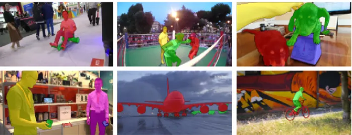
Figure 4.1: Davis 2017: A multi-instance video object segmentation dataset.
In chapter 3, video colorization was posed as a self-supervised learning problem for visual tracking. This chapter describes how the feature representations learned from colorization can be used as an unsupervised tracker. Subsequently, the tracker is quantitatively and qualitatively evaluated on the task of video object segmentation. Furthermore, graphical models specific to the task are applied to remove any artifacts and refine the results of the model. Significant improvements over the baseline are demonstrated.
4.1 TASK
The performance of the video tracker learned from colorization is evaluated against the DAVIS 2017 video object segmentation dataset [4]. It is a widely adopted benchmark in the community. The videos in the dataset are challenging and consist of multiple objects that undergo significant deformation, occlusion, and scale change with cluttered backgrounds.
The task of the challenge is to densely label one or more objects in every frame of the video for the semi-supervised scenario, i.e. the per-pixel segmentation mask of the first frame is given, and no human interaction or refinement is allowed.
The performance is evaluated by the F-1 measure of countour accuracy (F) and the Jaccard index (J), which is defined as the intersection-over-union of the estimated segmentation, M
and the ground-truth mask, G:
Note on Terminology: There is some disagreement in the tracking literature on nomenclature of what constitutes as semi-supervised and unsupervised tracking. There are two common tasks in visual tracking. In task A, the annotations for the first frame of the video are given. In task B, the annotations for the first frame are not given. The literature typically calls task A “semi-supervised” and task B “unsupervised” referring to whether the initial frame is labeled or not. The confusion in the terminology is that, in both cases, training with supervised data is permissible, even for the unsupervised task. However, our goal is to learn only from unlabeled video. At test time, we tackle task A, which specifies the region of interest to track. However, we call our method “unsupervised” because our model is trained without any ground-truth labels or fine-tuning for the task at hand.
4.2 BASELINE
We compare the performance of our unsupervised tracker on the DAVIS 2017 Challenge against the following unsupervised baselines:
Identity: Since we are given the ground-truth segmentation for the first frame of the test video, we have a baseline that assumes the video is static and repeats the initial segmentation for the rest of the video.
Optical Flow: We use two state-of-the-art methods in optical flow as a baseline [27, 63]. The first one is a classical optical flow implementation which is unsupervised and not learning based [63]. The second one is a learning based approach that learns from synthetic data [27]. In both cases, the target frames are estimated and the initial labels warped to produce the predicted segmentation. A pixel is labeled as belonging to a class if the warped score is above a threshold. Results achieved with the best performing threshold are reported. Both the recursive and non-recursive strategies are explored, and the strategy that works the best is reported. FlowNet2 [27] performs significantly better than classical optical flow. Therefore, unless otherwise stated, the reported results use FlowNet2 [27].
Fully-Supervised Models: The state-of-the-art supervised models with publicly available code are also considered to analyze the gap between our self-supervised model and fully supervised approaches [47, 64]. These models are trained on either of ImageNet [62], COCO [50], and DAVIS 2017 [4]. Furthermore, these supervised models are fine-tuned using the ground-truth segmentation of the first frame of the test videos.
4.3 TRACKING FROM COLORIZATION
Our model for self-supervised colorization produces embeddings that can be used to compute a similarity matrix A for any pair of target and reference frames. The similarity matrix can point from a pixel in the target frame to the most similar pixel in the reference frame(s). Albeit our model learns a “soft” pointer, one that gives the weights for linear combination of colors/labels in the reference frame(s) as shown in equation (3.2).
The colorization model is re-purposed for visual tracking/segmentation without any fine-tuning or additional training. To this end, we exploit the property of our model that it is non-parametric in the label space. The color vector in equation (3.2) is a one-hot vector
ci ∈Rd, wheredis the number of discrete color channels in the case of colorization. However,
the model does not place any restrictions on the dimensions of ci, nor does the ci have to be a one-hot vector. Moreover, the length of the vector d can change between learning and inference.
The label space can be any arbitrary discrete probability distribution of any number of random variables. Hence, the pointing mechanism learned from the task of colorization can be used to propagate labels through the entire video given an initially labeled frame. To this end, we simply re-use the equation (3.2) to propagate the distributions of categories rather than colors in the reference frame.
We re-interpret the labelci ∈ Rd as a vector indicating the probabilities for d categories.
For object segmentation, the categories correspond to individual instances in the video. The background counts as just another category. Since we know the ground truth labels for the first frame, its labels will be one-hot vectors, but the predictions in subsequent frames will be soft, indicating the confidence of the model. To make a hard decision, we choose the most confident category.
For video segmentation, the model takes a “hard” decision when it assigns labels. If the pointer is not confident, the predictions may be noisy and suffer from drift over time. To counteract this, the temperature of the softmax is adjusted to 0.5 during inference so that it makes more confident predictions. As with train time, the model propagates the labels from a window of N = 3 previous frames at test time as well.
4.4 DENOISING WITH MRFS
Our self-supervised tracker performs significantly better than unsupervised trackers that are not learning-based, especially for the types of motion characterized by occlusions and dynamic backgrounds. It is temporally more stable because of the temporal coherence of
color. However, the tracker has certain limitations. As the video progresses in time, the pointer becomes less and less confident as the distribution of labels draws closer. The problem is further aggravated when objects in the scene have similar structure and intensity to the region of interest. This leads to the formation of holes within and blobs outside of the region of interest.
To counteract and refine the segmentation, we leverage unsupervised graphical models. We use discrete Markov Random Fields (MRF) to denoise the segmentation masks during inference. This has the effect of smoothening the mask which fills the holes and removes undesirable blobs.
First, we describe the problem setting and a discrete MRF model adapted to denoising images. Then we formally derive a variational mean field method for approximate inference of the MRF model. We start with a simple Boltzmann machine for binary segmentation masks, and then extend it for denoising multi-label images.
4.4.1 Graphical Model
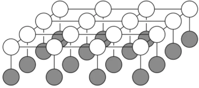
We define each pixel in the noisy image as an observed random variable X, and the unknown values of interest as H1, ..., HN. We perform maximum-a-posteriori (MAP) inference to find the values of H1, ..., HN that maximize P(H1, ..., HN|X). The model is formally intractable, so we exploit the natural context in images. A natural model is to assume that there are unknown, true pixel values H that tend to agree with the observed noisy pixel values X and with one another. So, our graph structure is defined as follows:
Figure 4.2: Discrete MRF for Image Denoising: The shaded nodes represent the observed pixel values Xi, and the open nodes represent the unknown, true pixel values Hi. EachXi is connected to the correspondingHi, and eachHi is connected to its neighborsHj. We obtain a discrete Markov Random Field (MRF) by placing a discrete random variable
Ui with a finite set of possible values at the ith node, and a coupling function θ(Ui, Uj) at edge from nodeitoj. We represent U as a one-hot vector. In a Boltzmann machine, which
we consider later, the binary random variable simply takes the value +1 or -1. In both cases, the coupling functions are defined as:
θ(Hi, Hj) = c (4.2)
θ(Hi, Xj) =kHi−Xjk (4.3)
4.4.2 Variational Inference
Since the MAP inference P(H|X) is intractable for our model, we use a variational inference approach that tries to find a tractable distribution Q(H; ˆθ) that is “close” to
P(H|X). A good choice of “close to” is to require that the KL-divergence of the two probability distributions, D(Q(H)kP(H|X)) be small. Although the KL-divergence is intractable, it is bounded by the variational free energy EQ, which can be evaluated.
EQ=EQ[logQ]−EQ[logP(H, X)] (4.4) Therefore, we obtain theQ(H) that minimizes theEQ, and as a result theQ(H) minimizes the KL-divergence as well. We use thatQ(H) as our approximation toP(H|X), and extract relevant information from Q(H).
4.4.3 Mean Field Method
We use the mean field method for variational inference. This approach assumes that Hi is conditionally independent of all others, and Q(H) comprises of a factor qi(Hi) for each hidden variableHi. Thus,Q(H) =q1(H1)q2(H2)...qN(HN). The iterative algorithm assumes that all but one of the terms inQ are known, and adjusts the remaining term.
For the simple case of a Boltzmann machine,qi(Hi) is a probability distribution over the two possible values ofHi, which are 1 and -1. If πi denotesP(Hi = 1), we have:
qi(Hi) = π (1+Hi) 2 i (1−πi) (1−Hi) 2 (4.5)
In order to minimize variational free energyEQ, we look at the two terms separately.
First, we consider the EQ[logQ] term:
EQ[logQ] =Eq1(H1)...qN(HN)[logq1(H1) +...+ logqN(HN)]
=Eq1(H1)[logq1(H1)] +...+EqN(HN)[logqN(HN)]]
(4.7) Next, we consider EQ[logP(H, X)]:
logp(H, X) = X i∈H X j∈N(i)∩H θijHiHj + X i∈H X j∈N(i)∩X θijHiXj +K (4.8)
Solving for the above equations gives us,
πi =
ea
ea+eb (4.9)
where the values of a and b are:
loga= X j∈N(i)∩H [θij(2πj−1)] + X j∈N(i)∩X [θijXj] (4.10) logb= X j∈N(i)∩H [−θij(2πj−1)] + X j∈N(i)∩X [−θijXj] (4.11)
For inference, each hidden node is visited iteratively, the associated πi is updated using the expression above assuming all the other πj are fixed, and this update rule is repeated until convergence is achieved.
The extension of the above method to multiple labels for discrete Markov Random Fields follows the same procedure. However, Ui is represented as a one-hot vector.
This gives us a more general form: loga= X j∈N(i)∩H [θijδ1(Hi, Hj)] + X j∈N(i)∩X [θijδ2(Hi, Xj)] (4.12)
Below, we outline the mean field inference algorithm for discrete MRF. We use the following notation in the below algorithm:
c= number of categories, which is number of instances + 1 for background
δ(x,y) = kx−yk, or the Frobenius norm
Data: Observed h×w image Result: Denoised h×wimage
c← number of objects + 1 πhw×c←0hw×c while δ(π, πprevious)< do πprevious ←π for i←1 to h×w do w← - P c([θ P j∈N(i,j)∩Hδ(πj, e(c))] +Pj∈N(i)∩X δ(Xj, e(c))) πi ←σ(w) end end
Algorithm 1: Mean field variational inference for discrete MRF
4.5 SEGMENTATION WITH GRAPH CUTS
Figure 4.3: Examples of GrabCut: The user drags a rectangle loosely around an object. The object is then extracted automatically. Image Courtesy: Rother et al. [2].
In the previous section, we use mean field variational inference to denoise the segmentation. However, an artifact of this smoothening is the expansion and blurring of the segmentation boundary. To counteract this undesirable side-effect, we iteratively extract the precise object segmentation using automatic “GrabCut” [2].
4.5.1 GrabCut
“GrabCut” is an image segmentation method based on graph cuts. Similar to other segmentation techniques “GrabCut” uses information encapsulated in the image. Most segmentation techniques make use of either the edge information or the region information in the image. However, “GrabCut” makes use of both edge and region information. This information is used to create an energy function which is minimized to produce the best segmentation.
In order to perform segmentation a graph is built, where nodes in the graph represent
node in the graph is connected to the Source and Sink node. The Source node represents the foreground of the image, and the Sink node the background. In order to segment the image the Source and Sink nodes must be separated.
The energy function is incorporated into the graph as weights between pixel nodes, and weights between pixel and Source or Sink nodes. Weights between pixel nodes are determined by edge information in the image. Thus, a strong indication of an edge between two pixels as measured by color gradient results in a very small weight between two pixel nodes. The region information determines the weights between pixels nodes, and the Source and Sink nodes. These weights are calculated by determining the probability of the pixel node being part of the background or foreground region.
In order for foreground and background regions to be created, some pixels in the image need to be labelled before segmentation as either certain foreground or background, which impose hard constraints on the model and the labels for these pixels are not altered.
Figure 4.4: Graphical Model for GrabCut: Each node in the graph represents pixels in the image. In addition, every pixel node in the graph is connected to the Source and Sink nodes, which represent the foreground and the background of the image respectively. A Min-cut/Max-Flow algorithm is used to extract the foreground from the background.
A Min-cut/Max-Flow algorithm is used to segment the graph. This algorithm determines the minimum cost cut that will separate the Source and Sink nodes. The cost of the cut is determined by the sum of all the weights of the links that are cut. Once the Source and Sink nodes are separated, all pixel nodes connected to the Source node become part of the
However, in our case we apply automatic “GrabCut” which does not require any user interaction. We apply erosion and dilation morphological operators on the segmentation from our self-supervised tracker to extract tri-maps for “GrabCut”.
4.6 RESULTS AND ANALYSIS
We evaluate our tracker for single-object as well as multi-object video segmentation tasks on the DAVIS 2017 Challenge. Our tracker achieves significant improvements over our chosen baselines. Our mean field inference approach fills in gaps in the region of interest, and removes any blobs, thereby improving segmentation recall. GrabCut refines segmentation boundary and improve precision as well as recall of contour accuracy.
Method Region Jaccard (J) Contour Accuracy F-1
Self-Supervised Tracker 49.48 49.02
Tracker with MFI 55.42 49.23
Tracker with MFI and GrabCut 60.05 52.2
Table 4.1: DAVIS 2016: Single-object video segmentation.
Method Region Jaccard (J) Contour Accuracy F-1
Identity 22.1 23.6
Optical Flow (Coarse-to-Fine) 13.0 15.1
Optical Flow (FlowNet2) 24.7 25.2
Our Self-Supervised Tracker 24.52 32.38
Tracker with MFI 24.69 33.49
Tracker with MFI and GrabCut 27.33 36.76
Table 4.2: DAVIS 2017: Multi-object video segmentation.
The largest improvement is recorded in recall. For both Intersection-over-Union (J) and Contour accuracy (F) measures, recall improves by 10-13% for both single and multi-object segmentation.
4.6.1 Jaccard Index and Contour Accuracy
measure for contour accuracy (F).
While optical flow makes strong predictions for motion vectors, warping the previous segment is error-prone due to occlusions, dynamic backgrounds, shaky camera motion and motion blur. In contrast, our model learns the tracker end-to-end on a large scale dataset. This has a regularizing effect since the unlabeled Kinetics video data will likely cover these challenging effects.
4.6.2 Temporal Stability
Analysis shows our approach maintains consistent performance for longer periods of time than optical flow. Optical flow based techniques accumulate errors over time. As we propagate color distribution, our model also suffers from drift. However, as we expect, color is temporally coherent for a longer span of time, whereas the performance of optical flow based trackers eventually degrades to the identity baseline.
4.6.3 Performance by Attributes
Our self-supervised tracker is more robust over optical flow for videos characterized by dynamic backgrounds and fast motion, which are traditionally challenging situations for optical flow. Training on large scale video dataset that includes these artifacts has a regularization effect on our learned model and hence, it is able to generalize better.
Since color has low spatial frequency, our tracker is able to handle situations involving occlusion and motion blur, which are difficult for optical flow because matching key-points is difficult under these conditions.
However, other known, stubborn problems such as scale variation, tracking small objects and lack of fine-grained details remain difficult. We believe these challenges can be resolved by operating at higher resolution feature maps and with improvements in colorization models.
Figure 4.5: Qualitative Evaluation: Figure shows ground truth annotation, our self-supervised tracker, and then results refined using MFI and GrabCut side-by-side.
CHAPTER 5: CONCLUSION
Our approach uses video colorization as a supervisory signal for learning to track. The self-supervised model leverages the temporal coherence of color to “manufacture” labels for colorization from large amounts of unlabeled video. The model learns spatiotemporal features that can be used as a pointer to propagate annotations from the initial frame as a reference to the rest of the video. We leverage this pointer for video object segmentation on the DAVIS 2017 dataset.
Experimental results show that our approach is more robust than the state-of-the-art optical flow-based unsupervised techniques. This holds true especially for motion types characterized by dynamic backgrounds, occlusions and motion blur. We attribute these improvements to the end-to-end training on diverse, large-scale data, which has a regularizing effect on the model and helps it generalize better.
Furthermore, we use non-parametric probabilistic graphical models to address the limitations of our unsupervised tracker. This results in additional improvements for both the intersection-over-union as well as the contour accuracy measures. The largest improvement is recorded in the recall for both the metrics.
However, illumination changes, scale variation, small objects and objects with fine-grained details present challenging situations for our model. Many of these problems may be addressed by simply increasing the resolution of the color features map.
Our results demonstrate that self-supervised video colorization can be a powerful signal for video analysis owing to the abundance of raw, unlabeled video on the web.
REFERENCES
[1] C. Vondrick, A. Shrivastava, A. Fathi, S. Guadarrama, and K. Murphy, “Tracking emerges by colorizing videos,” inProceedings of the European Conference on Computer Vision (ECCV), 2018, pp. 391–408.
[2] C. Rother, V. Kolmogorov, and A. Blake, “Grabcut: Interactive foreground extraction using iterated graph cuts,” in ACM transactions on graphics (TOG), vol. 23, no. 3. ACM, 2004, pp. 309–314.
[3] W. Kay, J. Carreira, K. Simonyan, B. Zhang, C. Hillier, S. Vijayanarasimhan, F. Viola, T. Green, T. Back, P. Natsev et al., “The kinetics human action video dataset,” arXiv preprint arXiv:1705.06950, 2017.
[4] J. Pont-Tuset, F. Perazzi, S. Caelles, P. Arbel´aez, A. Sorkine-Hornung, and L. Van Gool, “The 2017 davis challenge on video object segmentation,” arXiv preprint arXiv:1704.00675, 2017.
[5] C. Doersch, A. Gupta, and A. A. Efros, “Unsupervised visual representation learning by context prediction,” inProceedings of the IEEE International Conference on Computer Vision, 2015, pp. 1422–1430.
[6] A. Owens, J. Wu, J. H. McDermott, W. T. Freeman, and A. Torralba, “Ambient sound provides supervision for visual learning,” in European conference on computer vision. Springer, 2016, pp. 801–816.
[7] A. Owens and A. A. Efros, “Audio-visual scene analysis with self-supervised multisensory features,” inProceedings of the European Conference on Computer Vision (ECCV), 2018, pp. 631–648.
[8] D. Pathak, P. Krahenbuhl, J. Donahue, T. Darrell, and A. A. Efros, “Context encoders: Feature learning by inpainting,” in Proceedings of the IEEE conference on computer vision and pattern recognition, 2016, pp. 2536–2544.
[9] L. Jing, X. Yang, J. Liu, and Y. Tian, “Self-supervised spatiotemporal feature learning via video rotation prediction,” arXiv preprint arXiv:1811.11387, 2019.
[10] G. Larsson, M. Maire, and G. Shakhnarovich, “Colorization as a proxy task for visual understanding,” in Proceedings of the IEEE Conference on Computer Vision and Pattern Recognition, 2017, pp. 6874–6883.
[11] C. Vondrick, H. Pirsiavash, and A. Torralba, “Generating videos with scene dynamics,” in Advances In Neural Information Processing Systems, 2016, pp. 613–621.
[12] X. Wang and A. Gupta, “Unsupervised learning of visual representations using videos,” in Proceedings of the IEEE International Conference on Computer Vision, 2015, pp. 2794–2802.
[13] D. Pathak, R. Girshick, P. Doll´ar, T. Darrell, and B. Hariharan, “Learning features by watching objects move,” in Proceedings of the IEEE Conference on Computer Vision and Pattern Recognition, 2017, pp. 2701–2710.
[14] M. Noroozi and P. Favaro, “Unsupervised learning of visual representations by solving jigsaw puzzles,” in European Conference on Computer Vision. Springer, 2016, pp. 69–84.
[15] R. Zhang, P. Isola, and A. A. Efros, “Split-brain autoencoders: Unsupervised learning by cross-channel prediction,” in Proceedings of the IEEE Conference on Computer Vision and Pattern Recognition, 2017, pp. 1058–1067.
[16] X. Wang, K. He, and A. Gupta, “Transitive invariance for self-supervised visual representation learning,” in Proceedings of the IEEE International Conference on Computer Vision, 2017, pp. 1329–1338.
[17] C. Doersch and A. Zisserman, “Multi-task self-supervised visual learning,” in Proceedings of the IEEE International Conference on Computer Vision, 2017, pp. 2051– 2060.
[18] D. Jayaraman and K. Grauman, “Learning image representations tied to ego-motion,” in Proceedings of the IEEE International Conference on Computer Vision, 2015, pp. 1413–1421.
[19] P. Isola, J.-Y. Zhu, T. Zhou, and A. A. Efros, “Image-to-image translation with conditional adversarial networks,” in Proceedings of the IEEE conference on computer vision and pattern recognition, 2017, pp. 1125–1134.
[20] D. Xu, J. Xiao, Z. Zhao, J. Shao, D. Xie, and Y. Zhuang, “Self-supervised spatiotemporal learning via video clip order prediction,” in Proceedings of the IEEE Conference on Computer Vision and Pattern Recognition, 2019, pp. 10 334–10 343. [21] L. Pinto, D. Gandhi, Y. Han, Y.-L. Park, and A. Gupta, “The curious robot: Learning
visual representations via physical interactions,” in European Conference on Computer Vision. Springer, 2016, pp. 3–18.
[22] P. Agrawal, A. V. Nair, P. Abbeel, J. Malik, and S. Levine, “Learning to poke by poking: Experiential learning of intuitive physics,” in Advances in Neural Information Processing Systems, 2016, pp. 5074–5082.
[23] J. Wu, J. J. Lim, H. Zhang, J. B. Tenenbaum, and W. T. Freeman, “Physics 101: Learning physical object properties from unlabeled videos.” in BMVC, vol. 2, no. 6, 2016, p. 7.
[24] T. Zhou, M. Brown, N. Snavely, and D. G. Lowe, “Unsupervised learning of depth and ego-motion from video,” in Proceedings of the IEEE Conference on Computer Vision and Pattern Recognition, 2017, pp. 1851–1858.
[25] H.-Y. Tung, H.-W. Tung, E. Yumer, and K. Fragkiadaki, “Self-supervised learning of motion capture,” in Advances in Neural Information Processing Systems, 2017, pp. 5236–5246.
[26] T. Zhou, P. Krahenbuhl, M. Aubry, Q. Huang, and A. A. Efros, “Learning dense correspondence via 3d-guided cycle consistency,” inProceedings of the IEEE Conference on Computer Vision and Pattern Recognition, 2016, pp. 117–126.
[27] E. Ilg, N. Mayer, T. Saikia, M. Keuper, A. Dosovitskiy, and T. Brox, “Flownet 2.0: Evolution of optical flow estimation with deep networks,” in Proceedings of the IEEE conference on computer vision and pattern recognition, 2017, pp. 2462–2470.
[28] T. Zhou, S. Tulsiani, W. Sun, J. Malik, and A. A. Efros, “View synthesis by appearance flow,” in European conference on computer vision. Springer, 2016, pp. 286–301. [29] T. Welsh, M. Ashikhmin, and K. Mueller, “Transferring color to greyscale images,” in
ACM transactions on graphics (TOG), vol. 21, no. 3. ACM, 2002, pp. 277–280. [30] R. K. Gupta, A. Y.-S. Chia, D. Rajan, E. S. Ng, and H. Zhiyong, “Image colorization
using similar images,” in Proceedings of the 20th ACM international conference on Multimedia. ACM, 2012, pp. 369–378.
[31] X. Liu, L. Wan, Y. Qu, T.-T. Wong, S. Lin, C.-S. Leung, and P.-A. Heng, “Intrinsic colorization,” in ACM Transactions on Graphics (TOG), vol. 27, no. 5. ACM, 2008, p. 152.
[32] A. Y.-S. Chia, S. Zhuo, R. K. Gupta, Y.-W. Tai, S.-Y. Cho, P. Tan, and S. Lin, “Semantic colorization with internet images,” in ACM Transactions on Graphics (TOG), vol. 30, no. 6. ACM, 2011, p. 156.
[33] A. Deshpande, J. Rock, and D. Forsyth, “Learning large-scale automatic image colorization,” inProceedings of the IEEE International Conference on Computer Vision, 2015, pp. 567–575.
[34] R. Zhang, P. Isola, and A. A. Efros, “Colorful image colorization,” in European conference on computer vision. Springer, 2016, pp. 649–666.
[35] G. Larsson, M. Maire, and G. Shakhnarovich, “Learning representations for automatic colorization,” in European Conference on Computer Vision. Springer, 2016, pp. 577– 593.
[36] S. Guadarrama, R. Dahl, D. Bieber, M. Norouzi, J. Shlens, and K. Murphy, “Pixcolor: Pixel recursive colorization,” arXiv preprint arXiv:1705.07208, 2017.
[37] S. Iizuka, E. Simo-Serra, and H. Ishikawa, “Let there be color!: joint end-to-end learning of global and local image priors for automatic image colorization with simultaneous classification,” ACM Transactions on Graphics (TOG), vol. 35, no. 4, p. 110, 2016.
[38] R. Ironi, D. Cohen-Or, and D. Lischinski, “Colorization by example.” in Rendering Techniques. Citeseer, 2005, pp. 201–210.
[39] V. Badrinarayanan, F. Galasso, and R. Cipolla, “Label propagation in video sequences,” in 2010 IEEE Computer Society Conference on Computer Vision and Pattern Recognition. IEEE, 2010, pp. 3265–3272.
[40] S. Avinash Ramakanth and R. Venkatesh Babu, “Seamseg: Video object segmentation using patch seams,” in Proceedings of the IEEE Conference on Computer Vision and Pattern Recognition, 2014, pp. 376–383.
[41] S. Vijayanarasimhan and K. Grauman, “Active frame selection for label propagation in videos,” inEuropean conference on computer vision. Springer, 2012, pp. 496–509. [42] F. Perazzi, O. Wang, M. Gross, and A. Sorkine-Hornung, “Fully connected object
proposals for video segmentation,” inProceedings of the IEEE international conference on computer vision, 2015, pp. 3227–3234.
[43] M. Grundmann, V. Kwatra, M. Han, and I. Essa, “Efficient hierarchical graph-based video segmentation,” in 2010 ieee computer society conference on computer vision and pattern recognition. IEEE, 2010, pp. 2141–2148.
[44] C. Xu and J. J. Corso, “Evaluation of super-voxel methods for early video processing,” in2012 IEEE conference on computer vision and pattern recognition. IEEE, 2012, pp. 1202–1209.
[45] T. Brox and J. Malik, “Object segmentation by long term analysis of point trajectories,” in European conference on computer vision. Springer, 2010, pp. 282–295.
[46] K. Fragkiadaki, G. Zhang, and J. Shi, “Video segmentation by tracing discontinuities in a trajectory embedding,” in2012 IEEE Conference on Computer Vision and Pattern Recognition. IEEE, 2012, pp. 1846–1853.
[47] S. Caelles, K.-K. Maninis, J. Pont-Tuset, L. Leal-Taix´e, D. Cremers, and L. Van Gool, “One-shot video object segmentation,” in Proceedings of the IEEE conference on computer vision and pattern recognition, 2017, pp. 221–230.
[48] F. Perazzi, A. Khoreva, R. Benenson, B. Schiele, and A. Sorkine-Hornung, “Learning video object segmentation from static images,” in Proceedings of the IEEE Conference on Computer Vision and Pattern Recognition, 2017, pp. 2663–2672.
[49] J. Deng, W. Dong, R. Socher, L.-J. Li, K. Li, and L. Fei-Fei, “Imagenet: A large-scale hierarchical image database,” in 2009 IEEE conference on computer vision and pattern recognition. Ieee, 2009, pp. 248–255.
[50] T.-Y. Lin, M. Maire, S. Belongie, J. Hays, P. Perona, D. Ramanan, P. Doll´ar, and C. L. Zitnick, “Microsoft coco: Common objects in context,” in European conference
[51] A. Faktor and M. Irani, “Video segmentation by non-local consensus voting.” inBMVC, vol. 2, no. 7, 2014, p. 8.
[52] N. M¨arki, F. Perazzi, O. Wang, and A. Sorkine-Hornung, “Bilateral space video segmentation,” inProceedings of the IEEE Conference on Computer Vision and Pattern Recognition, 2016, pp. 743–751.
[53] A. Khoreva, R. Benenson, E. Ilg, T. Brox, and B. Schiele, “Lucid data dreaming for multiple object tracking,” arXiv preprint arXiv:1703.09554, 2017.
[54] D. Bahdanau, K. Cho, and Y. Bengio, “Neural machine translation by jointly learning to align and translate,” arXiv preprint arXiv:1409.0473, 2014.
[55] O. Vinyals, M. Fortunato, and N. Jaitly, “Pointer networks,” in Advances in Neural Information Processing Systems, 2015, pp. 2692–2700.
[56] V. Mnih, N. Heess, A. Graves et al., “Recurrent models of visual attention,” inAdvances in neural information processing systems, 2014, pp. 2204–2212.
[57] M. Jaderberg, K. Simonyan, A. Zisserman et al., “Spatial transformer networks,” in Advances in neural information processing systems, 2015, pp. 2017–2025.
[58] D. P. Kingma and J. Ba, “Adam: A method for stochastic optimization,”arXiv preprint arXiv:1412.6980, 2014.
[59] M. Abadi, P. Barham, J. Chen, Z. Chen, A. Davis, J. Dean, M. Devin, S. Ghemawat, G. Irving, M. Isard et al., “Tensorflow: A system for large-scale machine learning,” in 12th {USENIX} Symposium on Operating Systems Design and Implementation ({OSDI} 16), 2016, pp. 265–283.
[60] G. Bradski, “The OpenCV Library,” Dr. Dobb’s Journal of Software Tools, 2000. [61] K. He, X. Zhang, S. Ren, and J. Sun, “Deep residual learning for image recognition,” in
Proceedings of the IEEE conference on computer vision and pattern recognition, 2016, pp. 770–778.
[62] A. Krizhevsky, I. Sutskever, and G. E. Hinton, “Imagenet classification with deep convolutional neural networks,” in Advances in neural information processing systems, 2012, pp. 1097–1105.
[63] C. Liu et al., “Beyond pixels: exploring new representations and applications for motion analysis,” Ph.D. dissertation, Massachusetts Institute of Technology, 2009.
[64] L. Yang, Y. Wang, X. Xiong, J. Yang, and A. K. Katsaggelos, “Efficient video object segmentation via network modulation,” in Proceedings of the IEEE Conference on Computer Vision and Pattern Recognition, 2018, pp. 6499–6507.