Signalverarbeitung in der Erdbeobachtung
Regression-Induced Representation Learning and Its
Optimizer: A Novel Paradigm to Revisit Hyperspectral
Imagery Analysis
Danfeng Hong
Vollst¨andiger Abdruck der von der Ingenieurfakult¨at Bau Geo Umwelt der Technischen Universit¨at M ¨unchen zur Erlangung des akademischen Grades eines
Doktor-Ingenieurs (Dr.-Ing.) genehmigten Dissertation
Vorsitzender: Prof. Dr.-Ing. habil. Richard H. G. Bamler
Pr ¨ufer der Dissertation: 1. Prof. Dr.-Ing. habil. Xiaoxiang Zhu 2. Prof. Dr. Jocelyn Chanussot
3. Prof. Dr. Guisong Xia
Die Dissertation wurde am 23.05.2019 bei der Technischen Universit¨at M ¨unchen ein-gereicht und durch die Ingenieurfakult¨at Bau Geo Umwelt am 07.10.2019 angenommen.
Abstract
A
irborne and spaceborne hyperspectral imagery (HSI) is a remotely sensed 3D imag-ing product of stackimag-ing hundreds or thousands of 2D images finely sampled from the continuous wavelength covering the whole electromagnetic spectrum, i.e. 300nm-2500nm. A narrower swath width in spectral domain enables the HSI to discriminate the materials, particularly for those that are extremely similar in the range of visual light, at a more ac-curate level unachievable by easily-available multispectral or RBG imagery. Over the past decades, unprecedented progress in many challenging tasks of earth observation, such as mineral exploration, precision agriculture, and disaster responses, has been made by the means of HSI acquired by currently operational hyperspectral satellites (e.g., ASTER, Hy-perion, CHRIS) and advanced aerial imaging sensors (e.g., DAIS, ROSIS, HyMap, HySpex). Nevertheless, three crucial issues in HSI – the need for large storage capacity, the spec-tral variability caused by extrinsic factors (e.g., environmental conditions and instrumental configurations) and the intrinsic deformation of the materials, and small-scale availability due to the limitations of satellite devices itself – hardly make it applicable to a large-scale real scene. Our primary concern is supposed to, therefore, point-to-point addressing the aforementioned problems in order to better brace for upcoming or newly-launched spec-troscopy imaging missions, such as German EnMap, NASA’s HyspIRI, DLR’s DESIS, and Chinese Tiangong-1, Gaofen-5, Zhuhai-1, whose products will be possessed of higher spatial and spectral resolution, wider coverage area, shorter temporal sampling intervals, stronger mapping ability, but also larger storage need and tighter coupling between bands. For this purpose, the thesis will be unfolded from the three main aspects of hyperspectral remote sensing, includinghyperspectral dimensionality reduction,spectral unmixing, andcross-modality feature fusion and learning, with five algorithmic contributions to overcoming
thetrade-off between robustness and representation capability of HSI in a regression-based learning paradigm.
Inhyperspectral dimensionality reduction, thetrade-off between the explosively growing
spectral dimension and the spectral discrimination ability has been an emphatically-focused problem, in that very high dimensionality raises the information redundancy and also in-troduces more complex noise distribution. Inspired by the statistical robustness of regres-sion technique, a multi-layered regresregres-sion representation model is developed to improve the discriminative ability of which common regression models are lack 1) by jointly per-forming dimensionality reduction and classification; 2) by progressively searching several intermediate states of subspaces to approach an optimal mapping; 3) by spectrally embed-ding manifold structure in each learnt latent subspace in order to preserve the same or similar topological property between the compressed data and the original data.
There is another to-be-considered trade-off existed in spectral unmixing, that is, spectral variations and accurate unmixing. In this thesis, two feasible solutions to address the spec-tral variability are introduced by providing new insights into the inverse problem of hy-perspectral unmixing. The former assumes to be a low-coherence between real spectral sig-natures and spectral variabilities and then integrates this attribute into a sparse and dense joint regression model, called the augmented linear mixing model (ALMM). While for the latter, it seeks to unmix the HSI in a to-be-estimated subspace instead of in the original high-dimensional space, and the subspace and abundance maps in unmixing can be jointly optimized with a low-rank attribute embedding.
A rethinking-worthy open problem for the exiting and upcoming hyperspectral imaging missions ishow to use the HSI to contribute to a large area and even global mapping and mon-itoring, since there are higher spectral resolution yet lower spatial resolution and smaller coverage from space in these HSIs than those of MSIs. Thistrade-off between HSI and MSI
naturally leads to a challenging issue related to cross-modality feature fusion and learn-ing. With this intent, a regression-based cross-modality learning framework is designed, called common subspace learning (CoSpace), to linearly learn a shared latent subspace from hyperspectral-multispectral (HS-MS) correspondences by locally aligning the mani-fold structure of the two modalities. Through the learned subspace, the HSI’s properties can be effectively transferred into the MSI available on a larger scale. Beyond the CoSapce, a semi-supervised learning framework is proposed by learning to simultaneously align the data structures of labeled and unlabeled samples as well as multi-modalities in the form of graph representation.
Moreover, a unified optimizer followed by the alternating direction method of multipli-ers (ADMM) strategy is developed and generalized to solve the above-mentioned five algo-rithms.
Besides, these proposed strategies in different hyperspectral tasks have been proven to be superior and effective, from both visually and quantitatively, in comparison with other state-of-the-art methods for a variety of simulated and real data scenarios.
Zusammenfassung
L
uft- und raumfahrtgest ¨utzte Hyperspektralbilder (HSI) sind ein ferngesteuertes 3D-Bildgebungsprodukt, bei dem hunderte oder tausende 2D-Bilder stapelweise aus der kontinuierlichen Wellenl¨ange des gesamten elektromagnetischen Spektrums, d.H. von 300 nm bis 2500 nm, abgetastet werden. Eine geringere Streifenbreite im Spek-tralbereich erm¨oglicht eine genauere Unterscheidung von Materialien, welche mittels le-icht zug¨anglichen Multispektral- oder RGB-Bildern nle-icht erreichbar w¨are. Dies gilt ins-besondere f ¨ur Materialien, die sich im visuellen Spektrum stark ¨ahneln. In den letzten Jahrzehnten wurden mit Hilfe von “HSI”, von derzeit in Betrieb befindlichen hyperspek-tralen Satelliten (z. B. ASTER, Hyperion, CHRIS) und fortschrittlichen Luftbildsensoren (z.B. DAIS, ROSIS, HyMAP, HYSpex), beispiellose Fortschritte bei vielen anspruchsvollen Aufgaben der Erdbeobachtung erzielt, beispielsweise bei der Mineralexploration, der Pr¨azisionslandwirtschaft und bei der Katastrophenbew¨altigung.Dennoch erschweren drei entscheidende Punkte die Anwendbarkeit von HSI f ¨ur große reale Szenen. Diese umfassen 1) den Bedarf an großer Speicherkapazit¨at, 2) die spektrale Vari-abilit¨at durch ¨außere Faktoren (z.B. Umgebungsbedingungen und Ger¨atekonfigurationen) und 3) die Eigenverformung der Materialien, sowie die Verf ¨ugbarkeit im kleinen Maßstab durch die Einschr¨ankungen der Satellitenger¨ate selbst. Unser Hauptanliegen ist es da-her, die oben genannten Probleme punktuell anzugehen, um besser auf bevorstehende oder k ¨urzliche gestartete spektroskopische Bildgebungsmissionen-Missionen, wie German EnMap, HyspIRI der NASA, DESIS des DLR und chinesisches Tiangong-1, Gaofen-5 uund Zuhai-1 vorbereitet zu sein, dessen Produkte eine h¨ohere r¨aumliche und spek-trale Aufl¨osung, einen gr¨oßeren Erfassungsbereich, k ¨urzere zeitliche Abtastintervalle, eine st¨arkere Kartierungsf¨ahigkeit, aber auch einen gr¨oßeren Speicherbedarf und eine engere Verflechtung zwischen den B¨andern aufweisen werden. Zu diesem Zweck wird diese Dis-sertation aus den drei Hauptaspekten der hyperspektralen Fernerkundung entwickelt, ein-schließlichder Verringerung der hyperspektralen Dimensionalit¨at,der spektralen
Ent-mischung und der Kombination und des Lernens von Kreuzmodalit¨aten mit f ¨unf
al-gorithmischen Beitr¨agen zur ¨Uberwindung des Kompromisses zwischen Robustheit und Repr¨asentationsf¨ahigkeit von HSI in einem regressionsbasierten Lernparadigma.
Bei der Verringerung der hyperspektralen Dimensionalit¨at war der Kompromiss
zwis-chen der explosionsartig wachsenden spektralen Dimension und der spektralen Diskri-minierungsf¨ahigkeit ein nachdr ¨ucklich fokussiertes Problem, da eine sehr hohe Dimen-sionalit¨at die Informationsredundanz erh¨oht und auch eine komplexere Rauschverteilung einf ¨uhrt. Inspiriert von der statistischen Robustheit der Regressionstechnik wird ein mehrschichtiges Regressionsrepr¨asentationsmodell entwickelt, um die Diskrim-inierungsf¨ahigkeit zu verbessern, an der g¨angige Regressionsmodelle fehlen 1) durch gemeinsames Durchf ¨uhren der Dimensionsreduktion und -klassifizierung; 2) durch schrit-tweises Durchsuchen mehrerer Zwischenzust¨ande von Unterr¨aumen, um sich einer opti-malen Abbildung anzun¨ahern; 3) durch spektrales Einbetten einer Mannigfaltigkeitsstruk-tur in jeden erlernten latenten Unterraum, um die gleiche oder eine ¨ahnliche topologische Eigenschaft zwischen den komprimierten Daten und den urspr ¨unglichen Daten zu erhalten.
Bei der spektralen Entmischung gibt es einen weiteren Kompromiss zwischen spektraler
Variationen und genauer Entmischung. In dieser Arbeit werden zwei m¨ogliche L¨osungen zur Behebung der spektralen Variabilit¨at vorgestellt, indem neue Erkenntnisse ¨uber das in-verse Problem der hyperspektralen Entmischung bereitgestellt werden. Ersteres geht von einer niedrigen Koh¨arenz zwischen echten Spektralsignaturen und Spektralvariabilit¨aten aus und integriert dieses Attribut in ein sp¨arliches und dichtes Regressionsmodell, das als Augmented Linear Mixing Model (ALMM) bezeichnet wird. Letzteres versucht in einem zu
sch¨atzenden Unterraum statt im urspr ¨unglichen hochdimensionalen Raum zu entmischen, und die Unterraum- und Abundanzkarten beim Entmischen gemeinsam mit einer nieder-rangigen Attributeinbettung optimiert werden k¨onnen.
Ein umdenkenswertes offenes Problem f ¨ur die bestehenden und zuk ¨unftigen hyperspek-tralen Bildgebungsmissionen ist, wie man mit HSI zu einer großr¨aumigen und sogar glob-alen Kartierung und ¨Uberwachung beitragen kann, da f ¨ur HSI zwar eine h¨ohere spektrale Aufl¨osung als f ¨ur MSI erreicht werden kann, gleichzeitig jedoch eine geringerer r¨aumlicher Aufl¨osung und Abdeckung. DieserKompromisszwischen HSI und MSI f ¨uhrt naturgem¨aß zu einem herausfordernden Problem im Zusammenhang mitCross-Modality-Feature-Fusion
und Lernen. Mit dieser Absicht wird ein regressionsbasiertes
Cross-Modality-Learning-Framework entwickelt, das als Common Subspace Learning (CoSpace) bezeichnet wird, um einen gemeinsam genutzten latenten Unterraum aus hyperspektralen, multispektralen (HS-MS) -Korrespondenzen durch lokales Ausrichten der vielf¨altigen Strukturen der beiden lin-ear zu lernen Modalit¨aten. Durch den erlernten Teilraum k¨onnen die Eigenschaften des HSI effektiv in das MSI ¨ubertragen werden, welches in einem gr¨oßeren Maßstab verf ¨ugbar ist.
¨
Uber das CoSapce hinaus wird ein semi- ¨uberwachtes Lernframework vorgeschlagen, in dem die Datenstrukturen von markierten und nicht markierten Proben sowie Multimodalit¨aten in Form einer Diagrammdarstellung gleichzeitig abgeglichen werden.
Dar ¨uber hinaus wird ein einheitlicher Optimierer, gefolgt von der Strategie der alternieren-den Richtungsmethode der Multiplikatoren (ADMM), entwickelt und verallgemeinert, um die oben genannten f ¨unf Algorithmen zu l¨osen.
Zudem haben sich diese vorgeschlagenen Strategien f ¨ur unterschiedliche hyperspektrale Aufgaben sowohl visuell als auch quantitativ im Vergleich mit anderen modernen Meth-oden f ¨ur eine Vielzahl simulierter und realer Datenszenarien als ¨uberlegen und wirksam erwiesen.
List of Abbreviations
Abbreviation Description 1-D one-dimensional 2-D two-dimensional 3-D three-dimensional AA average accuracyACMSL alignment-based cross-modality share learning ADMM alternating direction method of multipliers
ALMM augmented linear mixing model
AVIRIS Airborne Visible / Infrared Imaging Spectrometer AutoRULe auto-reconstructing unsupervised learning
CASI Compact Airborne Spectrographic Imager
CCF canonical correlation forests
CDF cumulative distribution function
CD coordinate descent
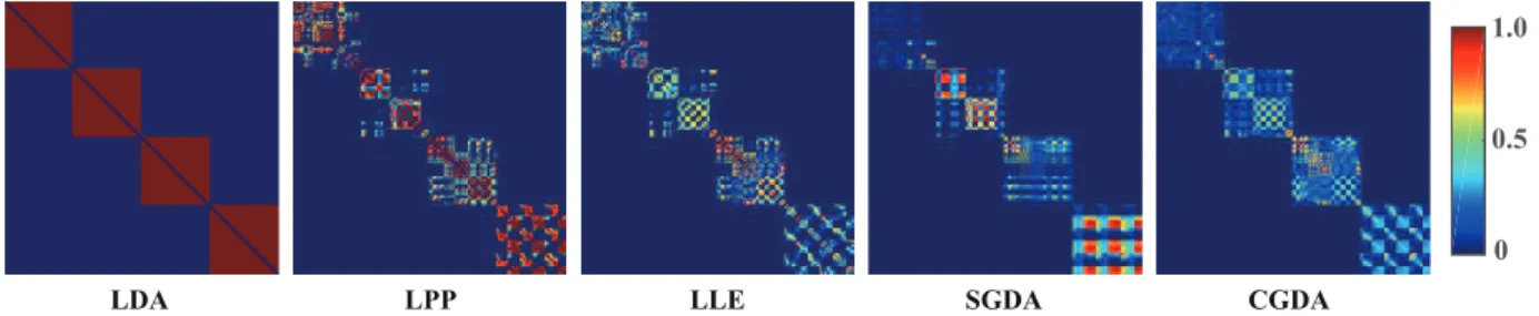
CGDA collaborative graph-based discriminant analysis
CML cross-modality learning
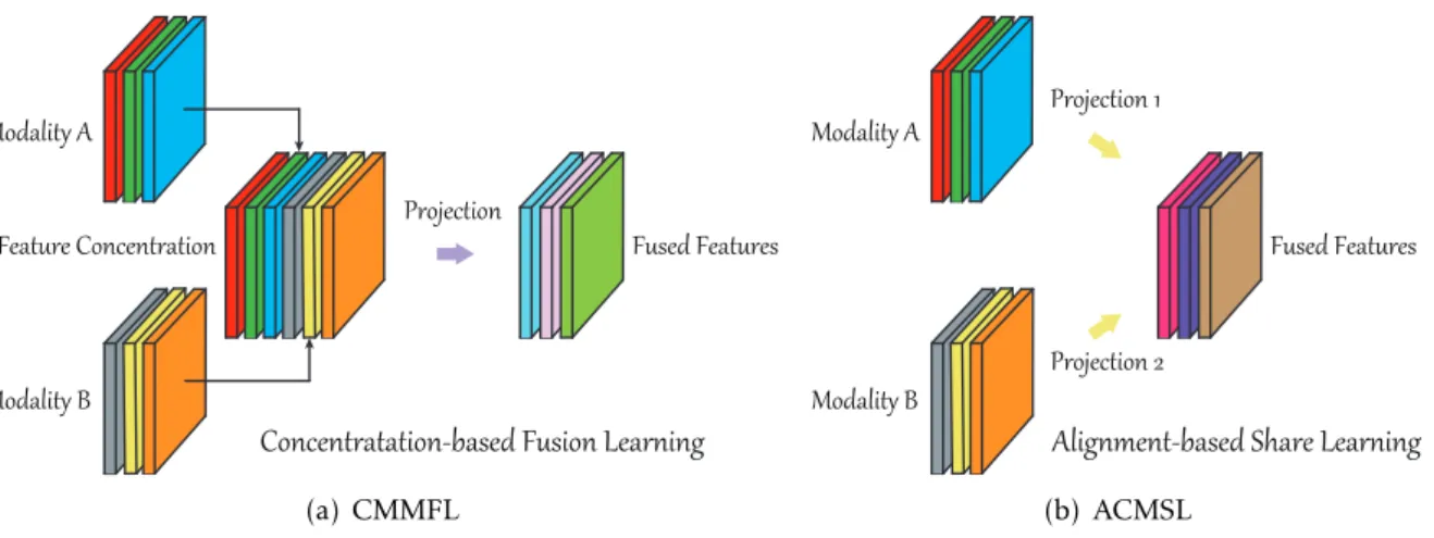
CMMFL concentration-based multi-modality fusion learning
CMs classification maps
CoSpace common subspace learning
DADR discriminant analysis dimensionality reduction DAIS Digital Airborne Imaging Spectrometer
DANSER dictionary-adjusted non-convex sparsity-encouraging regression DLR Deutschen Zentrums f ¨ur Luft- und Raumfahrt
ELMM extended linear mixing model
FA factor analysis
FCLUS fully constrained least squares unmixing FSDA feature space discriminant analysis
GBM generalized bilinear model
GDA graph-based discriminant analysis
GDN global data normalization
GED generalized eigenvalues decomposition
Abbreviation Description
GLP graph-based label propagation
GSD ground sampling distance
HDR hyperspectral dimensionality reduction
HNS hierarchical neighbor selection
HS hyperspectral
HSI hyperspectral imagery
HyMap Hyperspectral Mapper
ICA independent component analysis
IFOV instantaneous field of view
IT iterative thresholding
ISOMAP isometric feature mapping
JL joint learning
JN joint normalization
J-Play joint and progressive learning strategy
KCGDA kernel collaborative graph-based discriminant analysis
KDA kernelized discriminant analysis
KLD Kullback-Leibler divergence
KLDA kernel linear discriminant analysis KLFDA kernel local fisher discriminant analysis KPCA kernel principle component analysis
KSGDA kernel sparse graph-based discriminant analysis
LARS least angle regression
LDA linear discriminant analysis
LDN local data normalization
LE Laplacian eigenmaps
LeMA learnable manifold alignment
LFDA local fisher discriminant analysis
LLE locally linear embedding
LML local manifold learning
LMM linear mixing model
LPP locality preserving projections
LSDR least-squares dimension reduction
LSL latent subspace learning
L-SMA LPP-based supervised manifold alignment LSQMI least-squares quadratic mutual information
Abbreviation Description
LSQMID least-squares QMI derivative
LTSA local tangent space alignment
L-USMA LPP-based unsupervised manifold alignment
MA manifold alignment
MAP maximum a posteriori
MIVIS Multispectral Infrared and Visible Imaging
MMDA multi-modality data analysis
MS multispectral
MSI multispectral imagery
NASA National Aeronautics and Space Administration
NN nearest neighbor
NPE neighborhood preserving embedding
NS neighbor selection
OA overall accuracy
OSF original spectral features
PCA principle component analysis
PCLSU partial con-strained least squares unmixing
PGD proximal gradient descent
P-JDR PCA-based on joint dimensionality reduction PPCA probabilistic principal component analysis
PLMM perturbed linear mixing model
QP quadratic programming
RBF radial basis function
RIRL regression-induced representation learning RLMR robust local manifold representation
RNS refined neighbor selection
RTT radiative transfer theory
SAM spectral angle mapper
SAR synthetic aperture radar
S-CoSpace semi-supervised CoSpace
SELD semi-supervised local discriminant analysis SELF semi-supervised local Fisher discriminant analysis SGDA sparse graph-based discriminant analysis
SIR sliced inverse regression
Abbreviation Description
SLDA subspace linear discriminant analysis
SMI squared-loss mutual information
SNR signal to noise ratio
SPCLUS scaled partial constrained least squares unmixing SSDA semi-supervised discriminant analysis
S-SMA Semi-supervised supervised manifold alignment
SU spectral unmixing
SULoRA subspace unmixing with low-rank attribute embedding
SUnSAL sparse unmixing by variable splitting and augmented Lagrangian
TDA topological data analysis
TV total variation
SVD singular value decomposition
SVM support vector machine
SVT singular value thresholding
UAV unmanned aerial vehicle
List of Symbols
Abbreviation Description α regularization parameter β regularization parameter γ regularization parameter λ regularization parameter Λ Lagrangian multiplier C class labelCov covariance matrix
D degree matrix
E expectation
g0(•) derivative of functiong(•)
hv function with respect to the variablev
k the number of classes
L Laplacian matrix
ρ increasing rate of penalty parameterµ
Θ latent subspace projection
Schur-Hadamard (term-wise) product
./ element-wise (term-wise) division
p(•) probability distribution function
ri residual vector
R residual matrix
S2 variance
Sw within-class scatter matrix
Sb between-class scatter matrix
φk(•) theknearest neighbor of the variable•
t iteration
tr(•) trace of matrix•
(•)T transpose of matrix
µ penalty parameter
µmax upper bound of penalty parameterµ
η tolerated errors
Abbreviation Description
V projection matrix
W adjacency matrix
xi spectral signature ofi-thpixel (sample)
X unfolded hyperspectral image
X mean value of the variableX
yi class label ofi-thpixel (sample)
Y label matrix that consists ofyi
Yl one-hot encoded label matrix
zi low-dimensional embedding (vector)
Z low-dimensional embedding (matrix)
∂(•) partial derivative of variable•
(•)−1 inverse of matrix k•k1,1 L1norm of matrix
k•k2 L2norm of vector
k•kF Frobenius norm
Contents
Abstract i Zusammenfassung iii List of Abbreviations v List of Symbols ix 1 Introduction 11.1 Motivation and Challenges 1
1.2 Objectives and Research Focus 2
1.3 Skeleton of the Thesis 4
2 Basics 5
2.1 Get to Know the Hyperspectral Imaging 5
2.1.1 Imaging Principle 5
2.1.2 Hyperspectral Sensors 5
2.1.3 Scanning Techniques of Hyperspectral Acquisition 7
2.1.4 Spectral Signature 8
2.1.5 Material Miscibility and Spectral Variability 9
2.1.6 Applications and Role of Hyperspectral Remote Sensing in Earth
Observation 10
2.2 Regression Techniques and Their Optimizers 11
2.2.1 Linear Regression 11
2.2.2 Ridge (or Dense) Regression 13
2.2.3 Lasso (or Sparse) Regression 13
2.2.4 Low-rank Regression 15
2.2.5 Joint Regression 16
3 State-of-the-art in Hyperspectral Data Analysis 18
3.1 Hyperspectral Dimensionality Reduction 18
3.1.1 Priority-driven Unsupervised Dimensionality Reduction 19
3.1.2 Category-guided Supervised Dimensionality Reduction 24
3.1.3 Semi-supervised Strategy of Dimensionality Reduction 28
3.2 Spectral Unmixing 30
3.2.1 Linear Mixing Model and Its Variants 30
3.2.2 Nonlinear Mixing Models 33
3.3 Multi-Modality Data Analysis 35
3.3.1 Concentration-based Multi-Modality Fusion Learning 36
3.3.2 Alignment-based Cross-Modality Share Learning 37
4 Summary of the Work 41
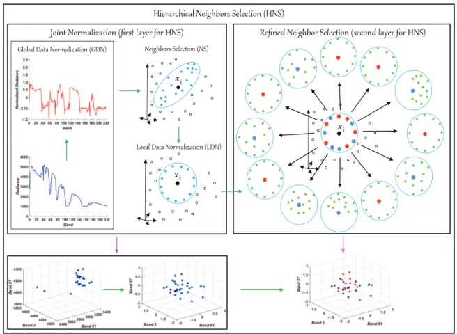
4.1 Robust Local Manifold Representation for HDR 41
4.1.1 Hierarchical Neighbors Selection 42
4.1.2 Spatial-Spectral Contextual Information Embedding 44
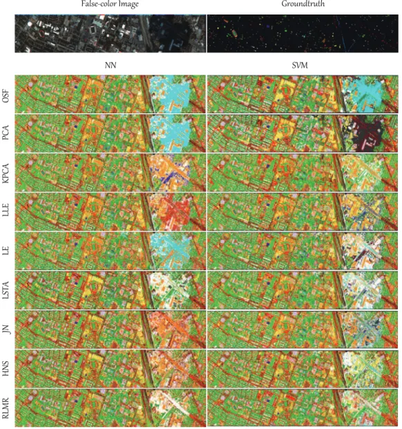
4.1.3 Performance Assessment: A Case of Classification 45
4.2 Joint & Progressive Learning of Hyperspectral Data 48
4.2.1 HDR from the View of Subspace Learning 49
4.2.3 Results and Analysis on Hyperspectral Data 52
4.3 Low-Coherence Learning for Hyperspectral Unmixing 53
4.3.1 Spectral Variability Modeling 54
4.3.2 Augmented Linear Mixing Model 56
4.3.3 Visualization of Unmixing Results 56
4.4 Low-Rank Subspace Unmixing: A Novel Strategy 58
4.4.1 General Remark in Subspace Unmixing 59
4.4.2 Low-rank Attribute Embedding 60
4.4.3 Visual Assessment of Abundance Maps 60
4.5 Learning Common Subspace across Multi- and Hyperspectral Modalities 63
4.5.1 Cross-Modality Learning in Remote Sensing 63
4.5.2 Learning to Align in the Latent Subspace 63
4.5.3 Larger Area Multispectral Classification with the Aids of HSI 66 4.6 Learnable Manifold Alignment in Cross-Modality: A Semi-Supervised Way 68
4.6.1 Data-Driven VS Hand-Crafted Graph Construction 69
4.6.2 Manifold Alignment Meets Graph Learning 70
4.6.3 Application in Cross-Modality Data Analysis 71
5 Conclusion and Outlook 76
5.1 Conclusion 76
5.2 Outlook 77
5.2.1 High-Efficiency and Low-Loss Hyperspectral Data Compression 77
5.2.2 Weakly-Supervised Learning-based Hyperspectral Unmixing 78
5.2.3 Evaluation of Spectral Unmixing: Build the Benchmark Datasets 78
5.2.4 Time-Series Hyperspectral Data Analysis 78
5.2.5 Geospatial Object Detection 78
References 79
Acknowledgement 93
Appendices 96
A Hong D., Yokoya N., Zhu X. X., 2017. Learning a Robust Local Manifold
Representation for Hyperspectral Dimensionality Reduction. IEEE Journal of Selected Topics in Applied Earth Observations and Remote Sensing
(JSTARS), 10(6): 2960-2975. 97
B Hong D., Yokoya N., Xu J., Zhu X. X., 2018. Joint & Progressive Learning
from High-Dimensional Data for Multi-Label Classification. European Conference on Computer Vision (ECCV), Munich, Germany, September,
pp. 469-484. 115
C Hong D., Yokoya N., Chanussot J., Zhu X. X., 2019. An Augmented Linear
Mixing Model to Address Spectral Variability for Hyperspectral Unmixing.
IEEE Transactions on Image Processing (TIP), 28(4): 1923-1938. 133
D Hong D., Zhu X. X., 2019. SULoRA: Subspace Unmixing with Low-Rank
Attribute Embedding for Hyperspectral Data Analysis. IEEE Journal of
E Hong D., Yokoya N., Chanussot J., Zhu X. X., 2019. CoSpace: Common Subspace Learning from Hyperspectral-Multispectral Correspondences. IEEE Transactions on Geoscience and Remote Sensing (TGRS), 57(7):
4349-4359. 167
F Hong D., Yokoya N., Ge N., Chanussot J., Zhu X. X., 2019. Learnable
Manifold Alignment (LeMA): A Semi-supervised Cross-modality Learning Framework for Land Cover and Land Use Classification. ISPRS Journal of
1
Introduction
1.1
Motivation and Challenges
H
yperspectral imaging, also known as imaging spectroscopy, is a seminal technique of truly achieving the integration of the 1-D spectrum and the 2-D image, which was first-ever to be conceptualized by Goetz1 et al. in 1980’s [Goetz et al., 1985]. From then on, hyperspectral remote sensing, which is evolved based on imaging spectroscopy, has garnered growing attention from researchers. Unlike those previous optical imaging tech-niques that sample the spectral space in a discrete (or very sparse) form (e.g., panchromatic, color photography, and multispectral imagery), the hyperspectral imaging systems exploit the senors to collect hundreds or thousands of spectral channels with an approximately continuous spectral sampling at a subtle interval (e.g., 10nm). This makes the hyperspec-tral remote sensing widely applied in earth observation and environmental surveys. More specifically, the main differences between hyperspectral remote sensing and those remote sensing techniques of low spectral resolution lie in the following three aspects:• The hyperspectral products are capable of finely discriminating the different classes
that belong to the same category, such as Citigroup Pine and American Giant Sequoia, Alunite and Kaolin. While for those traditional optical imaging products (e.g., multi-spectral imagery), they can only identify some materials with the significant differences in the spectral signatures, such as water, vegetation, soil, etc.
• The higher spectral resolution makes it feasible to some formerly impossible
applica-tions, e.g., parameter extraction of biophysics and biochemistry, automatic detection of food safety, which provides new insight into the field of the remote sensing technique.
• Due to the limitations in spectral and spatial resolution of imaging sensors,
atmo-spheric effects, and the interference of soil background, the traditional remote sensing technique was dominated by qualitative analysis. With the emergence of hyperspec-tral remote sensing, quantitative or semi-quantitative analysis is becoming increasingly possible.
Despite the HSI’s merits mentioned above, yet there are still several crucial issues that need to be sufficiently considered in the high-level data analysis with the use of HSI: information redundancy, spectral variability caused by illumination, topography change, atmospheric effects, and complex sensor noises, the need for large storage capacity and high performance computing, and data acquisition over a large area, among others. These drawbacks can be generalized to some specific challenges by raising three important questions about “ how” as follows:
• Overcoming the curse of dimensionality.As the HSI’s dimension gradually increases
along the spectral direction, the spectral discrimination ability in identifying the ma-terials would meet the bottleneck and even suffer from the degradation. This might be well explained by many possible factors, such as the coupling between the neighbor-ing spectral bands, more complex noise patterns, the same object with different spectra and different objects with the same spectrum. One challenge is posed to the first “how” question –how to effectively preserve the task-related information and get rid of the useless information in parallel?
• Addressing spectral variability. Due to the meter-level ground sampling distance
(GSD) of hyperspectral imaging, the spectral signatures for most pixels of HSI are ac-quired in the form of a complex mixture that consists of at least two types of
materi-als, inevitably degrading the performance of spectral identification. Spectral unmixing must be made before the high-level data analysis. However, the spectral variations, such as scaling factors, offsets, low-coherent or incoherent constituents, or complex noises, make it very difficult to accurately unmix these mixed pixels. Thus, the second “how” question corresponding to the challenge in spectral unmixing ishow to accurately esti-mate the abundance maps of the endmembers in the presence of spectral variability?
• Exploring and positioning the HSI’s role in future earth observation.There is an
ob-vious trend in the coming spaceborne earth observation, that is, extraordinary demand on global area data processing and analysis. It is well known, however, that a wealth of spectral bands enable the HSI to distinguish and detect the objects of interest with ease, especially for those spectrally similar classes, but its swath width from the space is completely incomparable to the one of optical broadband (e.g., multispectral) imag-ing due to the differences of imaging principles and techniques. For that reason, an application-innovative challenge in hyperspectral remote sensing is converted to de-scribing the third “how” question:how can HSI covering only a limited part of the MSI be explored to help improve the classification (or mapping) of the entire area covered by the MSI?
1.2
Objectives and Research Focus
With the coming of the “Big Data” era, large-scale remote sensing data management, mon-itoring and utilizing have developed into the mainstream in the next-generation earth ob-servation. As a central member of the remote sensing community, the HSI is duty-bound to participate in the tasks of global mapping, monitoring, and responding. Hence, the resulting general goal in this thesis is
“developing advanced algorithms to analyzing the hyperspectral data more robustly and efficiently with the potential contributions to improving the classification or mapping tasks in the
regional and even global coverage”.
Towards this goal, three main research objectives aiming at item-to-item handling the afore-mentioned challenges have been specified in the following:
− Objective 1:developing novel strategies to reduce the spectral dimension without sacrificing
the highly-discriminant information
Due to the highly-correlated characteristic between spectral bands, the HSI is subjected to the information redundancy, which could hurt the ability to discriminate the ma-terials under certain extremely-conditioned cases. Dimensionality reduction must be conducted before the high-level data analysis starts up. As a result, the first research branch of this thesis is to balance the spectral discrimination and robustness of the results before and after performing dimensionality reduction.
− Objective 2:discovering new prior knowledge against spectral variability for robust
hyper-spectral unmixing
In most previously-proposed unmixing models, e.g., the classic linear mixing model (LMM), they generally fail to consider the spectral variability in the process of esti-mating abundance maps. This leads to the poor unmixing performance by using those LMM-based approaches, since the spectral variability is not ignored or discarded but absorbed by the estimated abundances. To this end, the second investigated branch in the work is supposed to develop the new models linking with the spectral variability from the point of the physically-meaningful view.
multispectral data) to enhance the feature representation ability for preparation of large-scale land cover and land use classification.
Recently, multispectral spaceborne images are freely available on a nearly global scale, thanks to those optical broadband satellites that have been launched, such as Sentinel-2 [Drusch et al., Sentinel-201Sentinel-2], Landsat-8 [Roy et al., Sentinel-2014], etc. It should be noted, however, that limited by the spectral bandwidth, it is next to impossible for the multispectral data to distinguish the materials that are spectrally similar only with minute spectral discrepancies. In this connection, the final research branch of this dissertation is trans-ferring the highly-discriminant spectral information from HSI into wider-covered MSI of low spectral resolution only in the training phase, and improving the classification performance of the remaining large-scale MSI under the conditions without the corre-sponding HSI.
The traditional methodology of hyperspectral data analysis may not be qualified to cope with the above objectives. Consequently, the hyperspectral data analysis has to be revisited to find the technically feasible and theoretically-guaranteed solutions following an effective regression-based representation learning paradigm. Accordingly, the methodological focus of this thesis can be detailed as
− Solution 1:Docking to theObjective 1– hyperspectral dimensionality reduction task,
ajoint andprogressivelearning strategy(J-Play) is proposed to linearly find an optimal dimension-reduced subspace. The J-Play is made up of two strategies: the joint learn-ing that simultaneously performs subspace learnlearn-ing and regression aims at findlearn-ing a discriminative subspace by bridging the learned subspace with the label information, while the progressive learning gradually converts the original data space to a poten-tially optimal subspace through multi-coupled intermediate transformations, tending to find a better solution. Additionally, with the local manifold preservation on each intermediate subspace, the proposed method has demonstrated its robustness and dis-criminant capability as well as the ability to generalize the out-of-the-sample.
− Solution 2:Linking with theObjective 2, anaugmentedlinearmixingmodel (ALMM)
is proposed to view the spectral unmixing as a special case of bilinear mixing model by incorporating two different regression techniques: sparse regression attempting to accurately estimating the scaled abundance maps in the absence of other spectral vari-abilities, and dense regression allowing for reconstructing the rest of spectral variabili-ties except scaling factors with a to-be-updated spectral variability dictionary. The two parts can be organically coupled with a low-coherent assumption to be a joint model.
− Solution 3: Different from the Solution 2to solve the Objective 2, which unmixs the
HSI in the original spectral space, a novel subspace-based unmixing model is devel-oped with low-rank attribute embedding, called SULoRA, by jointly estimating sub-space projections and regressing the sparse abundance maps to robustify the inverse problems of hyperspectral unmixing against spectral variability.
− Solution 4: Connecting to theObjective 3, this thesis presents a general but effective
common subspacelearning method, CoSpace for short. Similarly to the J-Play in the So-lution 1, CoSpace also follows the joint learning framework. The main difference lies in that the latent subspace is learned by aligning the class-specific manifold structure of two modalities (MS-HS). Furthermore, through the subspace, the HSI-related proper-ties, e.g., high spectral discrimination, can be effectively transferred to those multispec-tral out-of-samples, thereby achieving the performance improvement of classification in a larger study scene.
of cross-modality learning, named as learnable manifold alignment (LeMA). As the name suggests, LeMA aligns the two different modalities not limiting to labeled data but also unlabeled data, by the means of data-driven learning strategy instead of the hand-crafted graph structure. Headed by the learned graph, the decision boundary may be better determined, i.e. using graph-based label propagation.
1.3
Skeleton of the Thesis
This is a cumulative dissertation to be unfolded around the general goal of hyperspectral imagery analysis, mainly including seven peer-reviewed papers – one top conference and six journal articles (please see the list of Appendix). The remainder of this thesis is guided as follows:
Chapter 2 starts with the introduction of hyperspectral imaging systems comprising imag-ing principle, the concept of spectral signals, and the explanation for material mixture and spectral variability as well as the potential applications in the next-generation earth obser-vation. Afterward, this chapter also makes a detailed review of several types of regression techniques and their solvers.
Chapter 3 systematically provides the analysis and discussion of the state-of-the-art meth-ods in hyperspectral data analysis from three main aspects: dimensionality reduction, spec-tral unmixing, and cross-modality feature fusion and learning. It then ends with clarifying our main contributions of this thesis.
Corresponding to these main contributions, the overview and summary of the seven rele-vant publications are given in Chapter 4, and the details in each paper can be found in the attached Appendix.
2
Basics
T
his chapter briefly makes a picture of hyperspectral imaging to help the readers who are interested or already in the field of hyperspectral remote sensing quickly acces-sible into the relevant topics. To begin with, the imaging principle is introduced and then its product is presented in the form of spectral signatures. Next, the material miscibility in HSI is explained by various factors and also spectral variability is pointed out to be ubiq-uitous. Finally, the role of hyperspectral remote sensing in earth observation and potential applications are clarified.2.1
Get to Know the Hyperspectral Imaging
2.1.1
Imaging Principle
Remote sensing [Tsang et al., 1985] is an important means of information acquisition in a contactless fashion. Technically speaking, it falls into “active” remote sensing, emitting the energy or signal by spacecraft or aircraft and receiving the response reflected from the object by the sensor similarly installed in spacecraft or aircraft, and “passive” remote sens-ing, which directly detects the radiation from the sunlight’s reflection on the surface of the Earth [Ulaby et al., 1986]. Figure 2.1 (a) and (b) illustrate the procedures of the two collec-tion patterns of remote sensing data. As a promising category of “passive” remote sensing, hyperspectral imaging [Goetz et al., 1985] judiciously assembles the two techniques of spec-troscopy and digital photography in a single system. The resulting product is a 3-D cube by simultaneously scanning the 2-D image plane in spectrally contiguous bands. The HSI holds a complete spectrum, which means that hundreds of (narrow) wavelength bands are collected at each pixel across the electromagnetic spectrum [Turner et al., 2003], i.e. from Gamma-rays, X-rays, the ultraviolet, through the visible and the infrared, to micro-waves, radio-waves, and even long-waves. Figure 2.1 (c) shows a fine partition for the electromag-netic spectrum.
2.1.2
Hyperspectral Sensors
As opposed to broad wavelength imaging techniques, such as RBG or multispectral imag-ing [Hong et al., 2015, Wu et al., 2019a, 2018], that provide the sparse spectral channels up to ten, imaging spectrometer uses the hyperspectral sensors, which is nothing struc-turally special with the charge-coupled device (CCD)-like and multispectral scanners but only difference in more spectral channels with the compacted sampling intervals, to record the detailed spectral information approximately being able to go throughout entire electro-magnetic spectrum. Up to the present, there has been an incrementally updating in imaging spectrometers from either aircraft or spacecraft, enabling the image quality progressively increasing. According to the different carriers, these sensors can be roughly categorized into two groups – airborne and spaceborne.
The former captures the imagery relatively flexibly due to the self-adapting to the schedule of image acquisition, which is effective to minimize the interference of changeable weather conditions caused by sum illumination, cloud blocking, and other atmospheric effects. The aircraft, also known as an unmanned aerial vehicle (UAV), helicopter, drone, airship, is of great benefit to developing a practical platform due to its flexibility in maintaining, re-pairing, and re-configuring the devices. A few of popular advanced airborne hyperspectral imagers will be briefly introduced, i.e.
Satellite (or Sensor) Solar (Lighting Source)
Forests Rocks Grass Built-up Area
Passive Remote Sensing
(a) Passive Remote Sensing
Satellite (or Sensor)
Forests Rocks Grass Built-up Area
Active Remote Sensing
(b) Active Remote Sensing
1000m 100m 10m 10cm 1cm 1mm 100μm 10μm 1μm 100nm 10nm 1nm 100pm10pm Wavelength 1017 1016 1015 1014 1013 1012 1011 1010 109 108 106 Frequency (Hz) 1018 1019 G am m a-ra ys X-rays U ltr av io le t Vi si bl e Microwaves Radiowaves Long waves 107 1m 1pm 1020 In!ared R ed O ra ng e Ye llo w G re en C ya n Bl ue Ind ig o Vi ol et 75 0n m 62 5n m 59 0n m 56 5nm 52 0n m 50 0n m 45 0n m 43 0n m 38 0n m N ea r I R Sh or t I R M ed iu m IR Lo ng IR Fa r I R 1.4µ m 3µ m 8µ m 15 µm 10 00 µm So ſt X-ra y H ar d X-ra y Su pe r H ar d X-ra y 1p m 10 pm 10 0p m 10 00 0p m 21 6M H z A M R ad io Sh or t w av e VH F TV 2 -6 FM R ad io VH F TV 7 -1 3 17 4M H z 88 M H z 54 M H z 0. 54 M H z 1.6 M H z Energy Increasing Wavelength Increasing (c) Electromagnetic spectrum
Fig. 2.1. An illustration to clarify the similarities and differences between “active” remote sensing and “passive” remote sensing [Tsang et al., 1985], as shown in (a) and (b). (c) gives a showcase of the electromagnetic spectrum [Turner et al., 2003]: the order from low to high according to frequency is Long-waves, Radio-waves, Micro-waves, Infrared, Visible, Ultraviolet, X-rays, and Gamma-rays, where several highlighted intervals, e.g., Radio-waves, Infrared, Visible, and X-rays are finely partitioned.
Airborne Visible / Infrared Imaging Spectrometer (AVIRIS) is a premier airborne
equipment used to measure the radiance in the spectral wavelength ranging from 400nm to 2500nm, which has been successively carried on four remote sensing plat-forms, e.g., NASA ER-2, de Havilland Canada DHC-6 Twin otters, Scaled Composites Model 281 Proteus, and NASA’s WB-57.
Compact Airborne Spectrographic Imager (CASI) is an instrument of recording the
ra-diance with at most 288 bands in the visible near Infrared (380nm to 1050nm) and of-fering 25cm spatial resolution. The hyperspectral cameras have contributed to a large number of applications of remote sensing, owing to its finer focus and the high sensi-tivity to lighting source.
Digital Airborne Imaging Spectrometer (DAIS-7915) collects the reflected radiance
across a wide range of spectral wavelength: 400nm to 12600nm, 79 channels in total. These channels are captured individually using four different Spectrometers that con-tain 32 bands (400nm to 1000nm), 8 bands (1500nm to 1800nm), 32 bands (2000nm to
Table 1. An overview of parameter configuration of several representative airborne hyperspectral sensors as well as oper-ational and upcoming spaceborne hyperspectral imaging missions where IFOV means instantaneous field of view. Some details stem from [Ortenberg et al., 2011].
Airborne Hyperspectral Sensors
Sensor Operator Spectral Range Band Number Spectral Resolution Spatial Resolution IFOV Swath
AVIRIS NASA 400-2500nm 224 10nm 17m 0.1mrad 11km
CASI ITRES 380-1050nm 288 2.5nm 0.25-1.5m 0.5mrad 1.5-7km
DAIS-7915 DLR 498-1010nm 32 16nm 3-20m 3.3mrad 2.5km 1500-1800nm 8 100nm 1970-2450nm 32 15nm 3000-5000nm 1 2000nm 8700-12300nm 6 600nm MIVIS SensTech 1100-1500nm 8 50nm 3-8m 2mrad 2.85km 1900-2500nm 64 9nm 8200-12700nm 10 35-45nm
HyMap HyVista 400-2500nm 128 15-20nm 3-10m 2.5mrad 1.7-6km
400-800nm 20 20nm
Spaceborne Hyperspectral Sensors
Sensor (Satellite) Altitude Spectral Range Band Number Spectral Resolution Spatial Resolution IFOV Swath
HIS (SIMSA) 523km 430-2400nm 220 20nm 25m 47.8urad 7.7km
Hyperion (EO-1) 705km 400-2500nm 220 10nm 30m 42.5urad 7.5km
CHRIS (PROBA) 580km 400-1050nm 19 1.25-11nm 25m 43.1urad 17.5km
MODIS (TERRA) 705km 400-1440nm 36 10-50nm 250-1000m 2000urad 2330km
HypSEO (MITA) 620km 400-2500nm 210 10nm 20m 40urad 20 km
Global Imager (ADEOS-2) 802km 380-1195nm 36 10-1000nm 250-1000m 310-1250urad 1600km
EnMAP 675km 420-1030nm 92 5-10nm 30nm 30urad 30km
950-2450nm 108 10-20nm
HyspIRI 700km 380-2500nm 200 10nm 60m 80urad 145km
2500nm) and 1 band (3000nm to 5000nm), and 6 bands (8000nm to 12600nm), respec-tively.
Multispectral Infrared and Visible Imaging (MIVIS): Similar to DAIS-7915, MIVIS,
which is a concurrent hyperspectral imaging system that operates from the visible to Thermal infrared ranges between 1100nm to 127000nm, covers three different wave-length ranges with 102 spectral channels.
Hyperspectral Mapper (HyMap) is manufactured in Australia, yielding four
spectrome-ters covering the spectral ranges of 400nm to 2500nm at a GSD of 5m. It is a well-known hyperspectral sensors that have been widely recognized in commercial circles.
More specifically, table 1 lists the parameter configuration of the above-mentioned hyper-spectral sensors in terms of the operator, hyper-spectral coverage, the number of hyper-spectral bands, spectral resolution, spatial resolution, and the instantaneous field of view. Furthermore, some operational and upcoming spaceborne hyperspectral missions (satellites) are also sum-marized in Table 1 with more detailed characteristics.
2.1.3
Scanning Techniques of Hyperspectral Acquisition
From the sampling point of the perspective, there are five types of basic ways to acquire the hyperspectral cube in hyperspectral imaging, they are point scanning, spatial scanning, spectral scanning, non-scanning (snapshot hyperspectral imaging), and spatio-spectral joint scanning, respectively. Figure 2.2 visualizes the five different scanning techniques in a 3-D
Point Scanning Spatial Scanning Spectral Scanning Non-Scanning Spatiospectral Scanning
Fig. 2.2. An evolutionary process of scanning techniques in hyperspectral imaging: five toy examples, from left to right, corresponding to point scanning, spatial scanning, spectral scanning, non-spanning, and spatio-spectral scanning, respec-tively.
toy sample of the hyperspectral cube.
Point Scanning, also known as whisk broom scanning, is a well-known technique of
passive remote sensing from aircraft or spacecraft, which has been extensively applied to obtain the aerial and satellite imagery. This possible reason to interpret this phe-nomenon is that the single detector in the whisk broom scanner only allows one pixel access to the lighting source each time. Although the resulting satellite products hold a high spatial resolution, yet such costly moving strategy burdens the sensor. Figure 2.2 illustrates the imaging process.
Spatial Scanning is a system of line-based scanning that uses the 2-D aperture
sen-sor to obtain slit-like spectra. The line scanning system is operated with a push broom scanner, which can be viewed as a variant of a whisk broom scanner. Thanks to the wider receptive field and longer scanning time, the push broom strategy tends to cap-ture more diversified light.
Spectral Scanning is also part of line scanning, yet the main difference with spatial
scanning is the spectrally scanning direction, which can be interpreted as a kind of spectral band-pass filters.
Non-Scanning outputs the entire hyperspectral cube in one shot because of without
any scanning operation. This greatly shortens the acquisition time of the image and meanwhile effectively avoids the motion artifacts caused by scanning. However, this is also a two-edged sword, since the snapshot benefits need to be supported by expen-sively computational cost.
Spatiospectral Scanning overcomes the drawbacks of the above line-based scanning
that only considers either spectrally or spatially moving direction at one time. By taking advantage of the dispersion technique, the scanning system is of benefit to generate the hyperspectral product of high spatial-spectral resolution.
It is worth mentioning that the specific application requirements guide the selection of scan-ning techniques.
2.1.4
Spectral Signature
Loosely speaking, spectral signature refers to the electromagnetic energy that is scattered, absorbed, transited and emitted from the surface of objects on the Earth, theoretically across any range of wavelengths. In hyperspectral imaging, the HSI is gathered with pixels each of which corresponds to a spectral signature that is quantified by vectors. The vector is a combinatorial radiance or reflectance, whose size is identical to the number of sampled spectral bands.
In view of the different reflectivity and absorptivity to various surface features on the ground, such as water, soil, forests and complex classes of land cover or land use, the de-tailed spectral signatures collected by hyperspectral sensors are capable of discriminating
Wavelength Wavelength R efl ec ta nc e R efl ec ta nc e Wavelength R efl ec ta nc e Vegetation Water
Asphalt & Soil & Vegetation
Building & Vegetation & Soil
}
}
}
}
Wavelength R efl ec ta nc e Wavelength R efl ec ta nc e Wavelength R efl ec ta nc eBuilding (70%) Vegetation (20%) Soil (10%)
=
+
+
Wavelength R efl ec ta nc e Wavelength R efl ec ta nc e Wavelength R efl ec ta nc e+
=
Asphalt (65%) Soil (30%) Pure Pixel Pure Pixel Mixed Pixel Mixed Pixel A Pure Pixel Grass: 0% Tree: 0% Sand: 0% Stone: 100% A Mixed Pixel Grass: 50% Tree: 25% Sand: 12.5% Stone: 12.5% Pure vs Mixed Wavelength R efl ec ta nc e+
Vegetation (5%)Fig. 2.3. A showcase in a real hyperspectral scene (Pavia City Centre) to quickly look at the concept of the hyperspectral image, spectral signature, and material mixture as well as pure pixel (endmember) and mixed pixel. The spectral signatures in the hyperspectral data are, as often as not, exhibited in the form of the reflectance, aiming to make the pixel spectral profiles comparable to some known materials. In the studied scene, the pure pixels correspond to two spectral reflectance curves of vegetation and water, respectively, while the mixed ones illustrate the case of spectral mixing, i.e. these mixed pixels consist of three components with different proportion. Furthermore, the right upper of the figure also gives two toy examples to explain the material miscibility.
and identifying the spectrally similar classes by capturing more subtle differences from the geometrically similar spectral shape. HSI can be usually seen as a stack of 2-D images con-tinuously acquired in the spectral direction. Figure 2.3 shows several examples of visualiz-ing spectral profiles in a real hyperspectral scene.
Besides, to correct the illumination, sensor devices, atmospheric effects, and solar and to-pographic compensation in the collection of remotely sensed digital images, radiometric calibration is an essential step in the data processing flow, yielding the calibrating spectral signatures.
2.1.5
Material Miscibility and Spectral Variability
Material mixing frequently occurs in hyperspectral imaging due to the inadequate spatial resolution in the image domain, or worse yet, intimate nonlinear interaction, which makes the recorded spectral signature commonly mixed at each pixel. This mixing behavior can be grouped into macroscopic mixing and microscopic mixing. Just as its name implies, the macroscopic mixture is an outcome by microscopically mixing multiple material compo-nents that come from the outside of the materials (or pixels), while for the microscopic mixture, the mixing process happens inside the materials (or pixels) in a nonlinear fashion. A showcase of material miscibility in a real city scenario with an illustration of toy examples (top-right corner) is given in Figure 2.3, where the mixing behavior happens in a pixel level and thus there are, more often than not, pure pixels and mixed pixels in a real-world hyper-spectral scene. For the former, only one material exists in the real ground area, which means that its percentage or abundance is 100%. Whereas the latter pixels are usually made up of two and more materials at a given GSD, hence their proportion can be computed according to the actual ground meters, e.g., there are four materials involved in a HSI’s pixel: Grass, Stone, Tree, and Sandwith the percentages of 50%, 12.5%, 25%, and 12.5%, respectively, as shown in Figure 2.3.
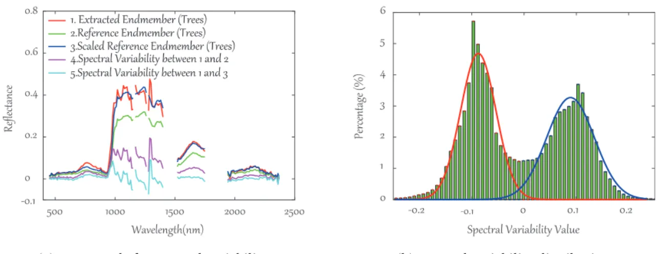
Due to the existence of material mixing behavior in HSI, the variation in the spectral signa-ture of material is inevitable. As shown in Figure 2.4, there is a visual example to clarify the spectral variability in a real hyperspectral scene. The factors may be multifarious, possibly
Spectral Bands 0 0.7 R efl ec ta nc e 0.6 0.5 0.4 0.3 0.2 0.1 0 20 40 60 80 100 120 Spectral Bands Sp ec tr al V ar ab ili ty 0.3 0.2 0.1 0 -0.1 -0.2 -0.3 -0.4 0 20 40 60 80 100 120 Spectral Bands R efl ec ta nc e 0.45 0.40 0.35 0.30 0.25 0.20 0.15 0.10 0.05 0 0 20 40 60 80 100 120 Trees A Hyperspectral Scene
(a) Spectral Signatures with Spectral Variability
(b) Pure Spectral Signature (c) Spectral Variablity
Fig. 2.4. A visual example of spectral variability in a real hyperspectral scene. A sub-area covering the trees is cropped to show the spectral variations in (a). (b) gives a smooth pure spectral signature for trees captured from the lab. It is clear to see from (c) the spectral variability between (a) and (b).
resulting from environmental, atmospheric, instrumental, physical or chemical effects. The spectral scaling, as a principal spectral variability, is frequently occurring, as the illumi-nation conditions, which are sensitive to the elevation and azimuth of the lighting source, result in the deformations of the topography and the changes of roughness in materials. Another important factor to bring the spectral variability is an atmospheric impact on the reflection, scattering or absorption of the electromagnetic energy when encountering vari-ous gases (e.g., carbon dioxide, oxygen), aerosol particles, water vapour, dust, to name a few. As explained above, the intimately mixing is also a leading source of spectral variability, which is given rise to the microscopically multiple scatting between-in the material. As a result, the robust estimation techniques [Hong et al., 2016a, 2014b] are needed to address the challenges.
2.1.6
Applications and Role of Hyperspectral Remote Sensing in Earth
Observation
Compared to on-site exploration, hyperspectral sensors record the information without the need to contact with the objects of interest. Together with the rich spectral information of HSI, hyperspectral remote sensing has gained growing attention in a wide range of applica-tions, not limiting to remote sensing, but including
Atmospheric and Hydrological Monitoring:Hyperspectral images have been viewed as a
powerful tool to detect the changes, e.g., in estimating aerosol density, tracking pollu-tion sources, mapping hydrological structure, analyzing gas constituents, and evaluat-ing water quality.
hyperspec-tral imaging [Feng and Sun, 2012, Gowen et al., 2007]. For example, the HSI can be used to inspect the freshness of the fruit and the concentrations of pesticides, owing to its spectral information that goes beyond the visible spectrum.
Forensic Medicine:Hyperspectral technique is apt to discover some tiny marks that are
easy to be ignored, such as remaining bloodstain, fiber differences, yielding the great support in the criminal cases.
Medical Diagnose:Highly spectral resolution makes it possible to timely detect the
dis-ease and obtain early treatment.
Energy Exploitation:Hyperspectral data are widely applied in the detection of oil and
toxic gas seeps, and it, on the other hand, also has the potential of exploiting the onshore and offshore petroleum, natural gas, minerals, and other energy sources.
Ecological Research:Hyperspectral images have been proven to be effective for the
bio-diversity investigation in the forest-covering area [Ghiyamat and Shafri, 2010] and the biomass and carbon estimation [Dube and Mutanga, 2016, Karila et al., 2019], i.e. by the means of the HSI-based classification.
Urban Planning and Management:Currently, a large number of researches have shown
the HSI’s superiority and effectiveness in a precise urban mapping (or classification) and change detection. This provides the researchers with a good foundation for the follow-up urban planning and management.
Still returning to the hyperspectral remote sensing of earth observation, the low spatial res-olution and small-scale data collection have been two main factors to limit the HSI to be a dominant role, in spite of great benefits to various applications. Fortunately, the Sentinel-1 SAR and Sentinel-2 multispectral satellites in operation allow largely and even globally SAR and multispectral data of high spatial resolution to be available. This naturally might deter-mine the role of the HSI that can become a significant complementary source to contribute to the large-scale earth observation tasks. That is to say, however, that the HSI is dispens-able; on the contrary, its highly discriminative spectral information is a key to unlock the bottleneck that SAR, multispectral, or other data sources fail to classify or recognize the ma-terials with fine-grained differences. As a result, this thesis not only presents the improve-ments targeting at some traditional challenges in hyperspectral data analysis, but also casts an interesting question related to cross-modality data analysis and proposes two advanced solutions.
2.2
Regression Techniques and Their Optimizers
Popularly speaking, the regression technique refers to utilizing the mathematically statis-tical method to measure or model the relations between dependent and independent vari-ables. According to the causality of describing the two variables, the regression technique can be further divided into linear regression analysis and nonlinear regression analysis. Among them, the linear regression is a frequently-used approach in practice, due to its easy-to-use style and ability to generalize well, while the nonlinear one is used to deal with more complex nonlinear relationships and its solution is usually obtained by solving an approximate linear regression problem. Combining with the main focus of this thesis in hy-perspectral data analysis, the following subsections will emphatically give priority to the linear regression-based techniques.
2.2.1
Linear Regression
From the machine learning perspective, the linear regression, a typical supervised learn-ing technique, aims at learnlearn-ing a function or model that could be any of a line, a
plane or a higher dimensional hyperplane by a linearized combination of different at-tributes. The learned model is expected to minimize the errors between the predicted and real values, thereby better generalizing the out-of-sample. Given a pair-wise training set {(x1,y1), . . . , (xi,yi), . . . , (xm,ym)} that contains the training samples X = {xi}m
i=1 ∈ Rb
×m with b dimensions (or bands) by m pixels (or samples) and corresponding class labels
Y = {yi}m
i=1 ∈ R1
×m
, yi ∈ {C1, C2, . . . , Ck}, where k denotes the number of classes, the
re-gression function or modelhv(•) can be written as
hv(xi) =v0+v1xi1+v2xi2+· · ·+vbxib, (2.1) making the to-be-estimated hv(xi) approach to yi. Eq. (2.1) can be also represented with vector ashv(xi) =Vxi, or with matrix ashV(X) =VX, where
V= [v0, v1, v2, . . . , vm]∈R1×b, X= [x0, x1, x2, . . . , xm]∈Rb×m, (2.2) andx0 = [1, 1,1, . . . , 1]T∈Rb×1. In order to assess the quality of the variableV, we need to define a following loss functionJ
J(V) =1 2 m X i (hv(xi)−yi)2= 1 2kVX−Yk 2 F= 1 2(XV−Y) T(XV−Y), (2.3)
wherek•kFdenotes the Frobenius norm. There are many strategies in minimizingJ(V) with
the respect to the variableV, written as min
V
J(V), such as least squares or gradient descend,
which are two commonly-used and effective algorithms.
Solution 1 – least squares:To facilitate the derivation, Eq. (2.3) can be unfolded as
J(V) = 1 2(XV−Y) T(XV−Y) = 1 2 h VTXTXV−VTXTY−YTXW+YTYi = 1 2 h VTXTXV−2WTXTY+YTYi. (2.4)
If and only if the input matrixX is full rank (m b), we then have the derivation of Eq.
(2.3):
∂J(V)
V =V
TXTX−XTY. (2.5)
Let Eq. (2.5) be equal to zeros, thus the variableVhas an analytical solution of (XTX)−1XTY
whenXTXis invertible .
Solution 2 – gradient descent:In more general cases, the gradient descend is used to solve
the problem (2.3) by searching the minimum. Note that due to the sensitivity to the initial point, the gradient descent algorithm could fall into a local minimum. More specifically, the gradient descend follows the following procedures:
1) initializing the variableVwith randomization or zero vector;
2) updating the variableV, making the value ofJ(V) reduced towards the direction of
gradient descent, according to the rule:
V←V−α∂J(V)
V , (2.6)
In this thesis, the full rank assumption of the matrixX is satisfied, thus the Solution 1 is preferable.
2.2.2
Ridge (or Dense) Regression
In reality, multicollinearity exits extensively between the data due to certain highly corre-lated vectors (or columns) in the matrix, particularly when the matrix is approaching singu-larity. To avoid the trivial solution or overfitting issue, the aforementioned ill-posed problem can be steadily and reliably solved by adding a regularization term parameterized byλ. This leads to a least-squares optimization problem with Tikhonov regularization, which can be formulated as min V 1 2kY−VXk 2 F+λkVk2F, (2.7)
whose closed-form solution is
V←(XTX+λI)−1XTY. (2.8)
Similarly, the variable Vin Eq. (2.7) can be optimized by gradient descent method with a modified update rule:
V←V(1−αλ)−α∂J(V)
V , (2.9)
where the penalty parameter λ controls the model’s complexity. As λ increases gradually, the absolute value of each element in the variable V tends to uninterruptedly decrease, further yielding a growing deviation relative to the actual V. This process could lead to a well-known underfitting, conversely call overfitting. Therefore, a proper λ may assist the model to reach a balance between robustness and fitting ability. In addition, due to the characteristic of theL2-norm, that is, each element in the estimatedVis a contributor to the
data fitting, the ridge regression is also called as dense regression or representation [Jiang and Lai, 2015].
2.2.3
Lasso (or Sparse) Regression
In ridge regression, the L2-norm constraint shrinks the to-be-estimated coefficients of the
variableVto a value close to zero but not exactly zero, which brings the difficulties in model understanding to a great extent, or in other words, is lack of physical meaning to explic-itly guide the variable (or feature) selection. What’s more, since the ridge regression has to estimate all elements of the variableV, even though a very small number, it still yields a computationally expensive cost. A straightforward and effective way to address the two problems is the least absolute shrinkage and selection operator (Lasso). By using L1-norm
penalty constraint in place ofL2-norm term in ridge regression, also known as sparse
re-gression [Bioucas-Dias et al., 2012], the resulting Lasso rere-gression can be represented in the form of a matrix as min V 1 2kY−VXk 2 F+λkVk1,1, (2.10)
wherekXk1,1 is defined as the sum of absolute values of each element of the matrixV,
for-malized byPm
i=1kxik1. SuchL1-norm may make many coefficients accurately converged to
zeros and reduce the effects of multicollinearity. Especially in the case – small-size sam-ples but high feature (variable) dimension, Lasso has been proven to be effective for high-dimensional statistic analysis by reducing the variations of the model and meanwhile in-creasing its regression precision.
Considering the non-differentiable points in L1-norm, the solvers, whether it be
least-squares or gradient descend, lose their functions. There have been some tailored optimiza-tion algorithms proposed for solving the Lasso problem, such as coordinate descent (CD),
Algorithm 1ADMM-based solver to Lasso (sparse) regression
Input: X,Y, and regularization parameterλ,maxIter
Output:the transformation vectorV
Initialize: Z1=V1=0,µ1= 10−3,µmax= 106,ρ= 1.5,t= 1,ζ= 10−4 1: whilenot converged ort >maxIterdo
2: Fix other variables to updateVt+1by solving a least-squares problem with Tikhonov
regularization
3: Fix other variables to updateZt+1by Eqs. (2.11) and (2.12) 4: Update Lagrange multipliers byΛt+1←Λt+µt(Zt+1−Vt+1) 5: Update penalty parameter byµt+1= min(ρµt, µmax)
6: Check the convergence condition: 7: ifkVt+1−Zt+1kF< ζthen 8: Stop iteration; 9: else 10: t←t+ 1; 11: Break; 12: end if 13: end while
least angle regression (LARS), proximal gradient descent (PGD), quadratic programming (QP), etc. These methods basically follow the iterative strategy and differ primarily in the heuristic mode, i.e. CD walks along the coordinate direction and LARS seeks to find the next-step points by maximizing the correlations with Cosine distance (corresponding to the least angle). Inspired by the iterative thresholding (IT) [Wright et al., 2009] that splits the problem (2.10) into two subproblems and then the sparse part (L1-norm: kVk1,1) can be
updated with a well-knownsoft-thresholding (shrinkage)operator [Chen et al., 2001]:
S←max{0,kV−Λ/µk1−λ/µ}sign(V−Λ/µ), (2.11)
wheresign(•) is defined by
sign(•) =
(
1, • 0
−1, • ≺0, (2.12)
the sparse regression problem in Eq. (2.10) can be effectively solved by embedding the soft-thresholding (shrinkage)operator into a general optimization framework based on the alter-nating direction method of multipliers (ADMM) [Bioucas-Dias and Figueiredo, 2010]. The general form of ADMM-based optimization problem is
min
V f(V) +g(V), (2.13)
whereV is the model parameter; f(V) and g(V) denote the loss function and the regular-ization term (i.e.g(V) =kVk1,1), respectively. Separating theg(V) from the overall objective
function, the Eq. (2.13) can be then rewritten by replacing the variableVofg(V) with a new variableZ:
min
V f(V) +g(Z), s.t. V
−Z=0.
(2.14) To relax the equality constraints of Eq. (2.14), the corresponding augmented Lagrangian function can be written as
LD(V,Z,Λ) =f(V) +g(Z) +ΛT(V−Z) +
µ
2kV−Zk
2
F, (2.15)