A Framework for Analyzing Stochastic Optimization Algorithms Under Dependence

(1)

A Framework for Analyzing Stochastic

Optimization Algorithms Under

Dependence

Chaoxu Zhou

Submitted in partial fulfillment of the requirements for the degree of

Doctor of Philosophy under the Executive Committee of the Graduate School of Arts and Sciences

COLUMBIA UNIVERSITY

(2)

(3)

ABSTRACT

A Framework for Analyzing Stochastic Algorithms Under Dependence

Chaoxu Zhou

In this dissertation, a theoretical framework based on concentration inequalities for empirical processes is developed to better design iterative optimization algorithms and analyze their

convergence properties in the presence of complex dependence between directions and step-sizes. Based on this framework, we proposed a stochastic away-step Frank-Wolfe algorithm and a stochastic pairwise-step Frank-Wolfe algorithm for solving strongly convex problems with polytope constraints and proved that both of those algorithms converge linearly to the optimal solution in expectation and almost surely. Numerical results showed that the proposed algorithms are faster and more stable than most of their competitors.

This framework can be applied for designing and analyzing stochastic algorithms with adaptive step-sizes that are based on local curvature for self-concordant optimization problems. Notably, we proposed and analyzed a stochastic BFGS algorithm without line-search, and proved that it converges linearly globally and super-linearly locally using the framework mentioned above. This is the first work that analyzes a fully stochastic BFGS algorithm, which also avoids time

consuming or even impossible line-search steps.

A third class of problems that the empirical processes framework can be applied to is to study the optimization of compositions of stochastic functions. A multi-level Monte Carlo based unbiased gradient generation method is introduced into stochastic optimization algorithms for minimizing function compositions. Based on this, standard stochastic optimization algorithms can be applied to these problems directly.

(4)

List of Tables

3.1 Comparisons of algorithms in terms of their requirements and theoretical perfor-mance to get an-approximate solution. In Table 3.1, FG denotes full gradient; SG denotes stochastic gradients; and LO denotes linear optimizations. In Prox-SVRG, mis the number of iterations in each epoch. In PSFW,|V|is the number of vertices in the polytope constraint. . . 17 3.2 Parameter choices in the algorithms . . . 34

(9)

List of Figures

3.1 Comparison between algorithms on simulated data. . . 34 3.2 Comparisons between algorithms on million song dataset. . . 36

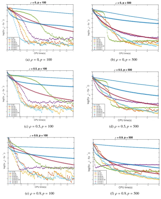
4.1 Experimental results for p = 100,500 and varying ρ. The x-axis is the elapsed CPU time and they-axis measureslog(f(x)− f(x∗)). . . 69

5.1 Performance plots for different algorithms on Cox’s partial likelihood dataset. . . . 125 5.2 Performance plots for different algorithms on the OCR dataset. . . 127

(10)

Acknowledgements

First and foremost, I would like to express my sincere gratitude to my academic advisors Professor Donald Goldfarb and Garud Iyengar. This thesis would not have been possible without their constant guidance and support during my graduate study. They not only provided valuable advice on my research, but also cared about my personal and career development, for which I am truly indebted and grateful.

I would also like to thank my committee members, Professors John Wright, Henry Lam, and Krzysztof Choromanski for their advice and helpful insights, and for careful reading of my thesis manuscript.

I would like to thank all the faculty and staff members of the Department of Industrial Engineering and Operations Research for creating such a supportive community. I am also obliged to my friends and fellow students for their sincere friendship.

I especially thank my family for their unconditional support and understanding throughout the years.

(11)

Chapter 1: Introduction and Background

1.1 Overview

In the era of big data, the main challenge that the field of optimization faces is the trade-off between solution accuracy and algorithm running time. To address this issue, a large number of stochastic optimization algorithms have been developed, especially for convex problems. When the directions and step sizes are both stochastic and depend on each other, analyzing the convergence properties of such algorithms poses great technical difficulty. To address this issue, we developed a theoretical framework based on concentration inequalities for empirical processes to better design algorithms and analyze their convergence properties in the presence of complex dependence.

Based on this framework, we proposed a stochastic away-step Frank-Wolfe algorithm and a stochastic pairwise-step Frank-Wolfe algorithm in [1] for solving strongly convex problems with polytope constraints and proved that both of them converge linearly to the optimal solution in expectation and almost surely. Numerical results showed that the proposed algorithms are faster and more stable than most of their competitors.

Another important issue for current stochastic optimization algorithms is step-size tuning. Most currently available stochastic algorithms are provably convergent only if either diminishing or in-finitesimal step-sizes are used. As a result, practitioners have to put a lot of effort into tuning step-sizes and other parameters in most of the algorithms that are used. To address this topic, we proposed an adaptive step-size framework based on local curvature for a number of stochas-tic algorithms for self-concordant optimization problems in [2]. Most notably, we proposed a stochastic BFGS algorithm without line-search, and proved that it converges linearly globally and super-linearly locally using the techniques mentioned above that we developed to resolve the de-pendence issue. This is the first work that analyzes a fully stochastic BFGS algorithm, which also

(12)

avoids time consuming or even impossible line-search steps.

A third class of problems that we studied addresses the optimization of compositions of stochas-tic functions. Problems that have this structure arise in many statisstochas-tics and machine learning appli-cations, such as parameter estimation for conditional random fields and for maximizing the partial likelihood in proportional-hazards models. In these problems, obtaining a stochastic gradient is already computationally difficult. Therefore most current approaches use biased stochastic gradi-ents in their algorithmic design, which results in non-optimal iteration complexities. To solve this problem, we introduced multi-level Monte Carlo methods into optimization algorithms for mini-mizing function compositions in [3]. We proposed simulation algorithms that generate unbiased gradient estimates with finite variance and finite expected computational cost. As a result, standard stochastic optimization algorithms can be applied to these problems directly. We also modified our simulation algorithms to enable them to incorporate various acceleration schemes.

1.2 The Empirical Processes Framework

Empirical processes generalizes the Glivenko-Cantelli theorem and the Donsker theorem to more general function classes. It has been widely used in analyzing large-sample properties of statistical estimators, especially M-estimators, in parametric, non-parametric, and semi-parametric statistical models. The uniform convergence results in the theory of empirical processes natu-rally resolve the complex dependence between the estimator and the samples when analyzing its properties. The complexity of the underlying function class, which is measured by the covering number, packing number, or bracketing number, plays an important role in the development of empirical processes theory. However, this set of tools has not been previously used in analyzing the properties of stochastic optimization algorithms. In chapter 2 of this thesis, we propose and develop a theoretical framework that is based on concentration inequalities for empirical processes for proving the convergence results for stochastic optimization algorithms under dependence.

(13)

1.3 The Frank-Wolfe Algorithm and Its Variants

The Frank-Wolfe algorithm, which is also known as the conditional gradient algorithm, was proposed in 1956 to minimize a convex function over a convex and compact feasible region. More specifically, for solving minx∈DF(x), where F(·) is a convex function and D is a convex and

compact set, the Frank-Wolfe algorithm proceeds as follows:

Algorithm 1The Frank-Wolfe Algorithm

Input:Initial solution x(1) ∈ D.

for k =1,2, . . .do

Set p(k) =arg mins∈Dh∇F(x(k)),si.

Setd(k) = p(k) −x(k).

Set x(k+1) = x(k) +γ(k)d(k), whereγ(k) = _k2₊₂ or obtain by line-search.

end for

Return: x(k+1).

The Frank-Wolfe Algorithm has become popular recently because it performs a sparse update at each step. For a good review of what was known about the FW algorithm until a few years ago, see [4]. When the feasible regionD is a polytope, it is well-known that this algorithm converges sub-linearly with rateO(1/k) because of the so-called zig-zagging phenomenon [5]. Especially if the optimal solutionx∗does not lie in the relative interior ofD, the FW algorithm tends to zig-zag

amongst the vertices that define the facet containing x∗. One way to overcome this zig-zagging

problem is to keep track of the "active“ vertices (the vertices discovered previously in the FW algorithm) and move away from the “worst” of these in some iterations. The Away-step Frank-Wolfe algorithm (AFW) and the Pairwise Frank-Frank-Wolfe algorithm (PFW) in [5] are two notable variants based on this idea.

In chapter 3 of this thesis, we will discuss in details and analyze the convergence properties of stochastic versions of these two algorithms. Moreover, in large-scale numerical experiments, the proposed algorithms perform as well as or better than their stochastic competitors in actual CPU

(14)

time.

1.4 Local Curvature Based Adaptive Step-size Algorithms

Many stochastic algorithms have been proposed to solve the generic stochastic optimization problem

min

x∈Rd

Eξf(x, ξ), and its finite sample version

min x∈Rd 1 n n X i=1 f(x, ξi),

including stochastic gradient descent (SGD), and variance-reduced extensions of SGD, such as SVRG [6], SAG [7], and SAGA [8]. These first-order methods extend gradient descent to the stochastic setting. It is natural to consider stochastic extensions of quasi-Newton and second-order methods. One such method, the Newton Incremental Method (NIM) [9], combines cyclic updating of a fixed collection of functions f(x, ξ1), . . . , f(x, ξm) with Newton’s method, and attains local superlinear convergence.

One of the key obstacles in developing stochastic extensions of quasi-Newton methods is the necessity of selecting appropriate step sizes. The analysis of the global convergence of the BFGS method [10] and other members of Broyden’s convex class [11] assumes that Armijo-Wolfe inexact line search is used. This is rather undesirable for a stochastic algorithm, as line search is both computationally expensive and difficult to analyze in a probabilistic setting. However, there is a special class of functions, the self-concordant functions, whose properties allow us to compute an adaptive step size based on local curvature and thereby avoid performing line searches. In [12], it is shown that the BFGS [13][14][15][16] method with adaptive step sizes converges superlinearly when applied to self-concordant functions.

In chapter 4 of this thesis, we will introduce class of stochastic, adaptive methods for mini-mizing self-concordant functions which can be expressed as an expected value. These methods generate an estimate of the true objective function by taking the empirical mean over a sample

(15)

drawn at each step, making the problem tractable. The use of adaptive step sizes, which are based on local curvature, eliminates the need for the user to supply a step size. Methods in this class include extensions of gradient descent (GD) and BFGS. Based on the empirical processes frame-work, we can show that, given a suitable amount of sampling, our stochastic adaptive GD method attains linear convergence in expectation, and with further sampling, our stochastic adaptive BFGS method attains R-superlinear convergence.

1.5 Unbiased Simulation Method for Stochastic Composition Optimization Problems

Most of the algorithms for solving the generic stochastic optimization problem,

min

x∈DEξf(x;ξ),

implicitly assume the gradient of each member function f(·;ξ) is easy to compute. But this as-sumption does not hold in the so-called stochastic composition optimization (SCO) problem [17]:

min

x∈DF(x) , Evfv(Ewgw(x)),

where v and w are random variables with certain known joint distributions nor its finite sample version: min x∈DFn(x) , 1 n n X i=1 fi{ 1 mi mi X j=1 gi j(x)}. (1.1)

As far as we know, all current algorithms that are used to solve SCO problems are based onbiased stochastic gradient oracles.

In chapter 5 of this thesis, we introduce unbiased gradient simulation algorithms that are based on a multilevel Monte Carlo technique for solving smooth SCO problems. Based on our unbiased gradient simulation algorithms, a stochastic composition optimization problem can be considered as a generic stochastic optimization problem.

(16)

Chapter 2: An Empirical Processes Framework

2.1 The Framework

The goal of developing the empirical prcoesses framework described in this section is to unify the convergence analysis of stochastic optimization algorithms under dependence. These results originate in empirical process theory [18]. The problem to be minimized has the form

min

x∈Rd

F(x) ≡_Eξf(x, ξ). (2.1)

We require the following assumptions onF and f for the analysis.

Assumptions:

1. There exist compact sets D₀ and D with x∗ ∈ D and D₀ ⊆ D ⊂ _Rd, such that if x₀ is chosen inD₀, then for all possible realizations of the samplesξ1, . . . , ξm(k) for every k, the

sequence of iterates {xk}∞_k₌₀ produced by the algorithm is contained within D. We write D= sup{kx−yk : x,y ∈ D }for the diameter ofD.

Furthermore, we assume that the objective values and gradients are bounded:

u= sup ξ xsup∈D f(x, ξ) < ∞ l = inf ξ xinf∈D f(x, ξ) > −∞ γ = sup ξ xsup∈D k∇f(x, ξ)k < ∞

2. There exists0 < L < ∞, such thatsup_ξ|f(x, ξ)− f(y, ξ)| < Lkx−yk.

(17)

sub-sampled functionF(k)(x) fromF(x).

Theorem 2.1.1. Let m(k) ∈_N+, and F(k)(x) ≡ 1

m(k) Pm(k) i=1 f(x, ξ (k) i ), whereξ (k) 1 , . . . , ξ (k) m(k) are i.i.d.

following the distribution ofξ. For any δ >0and0< < min{D,_2Lδ }, we have

P(sup x∈D |F(k)(x)−F(x)| ≥ δ) ≤ 2dd/2D d d exp ₋ m (k)₍_δ₋₂_L₎2 2(u−l)2 . (2.2)

Moreover, let x∗ =arg minx∈DF(x)and x∗(k) = arg minx∈DF(k)(x). For m(k) ≥ 3, we have

Based on this theorem, we are ready to state our theoretical framework for proving the con-vergence of stochastic algorithms. Let {y(k)} be a sequence of iterates that are generated by an iterative and deterministic algorithm which solves problem (2.1). Assume the iterates satisfies the property that

F(y(k+1))−F(y∗) ≤ ρ(k){F(y(k))−F(y∗)}, (2.5)

(18)

properties such as iteration count and hyper-parameters. Now consider a stochastic version of the deterministic algorithm which uses an average i.i.d. sub-sampled quantity to substitute for the original deterministic quantity. Let {x(k)}be the sequence of iterates generated by this stochastic algorithm. Then we have

F(x(k+1))−F(x∗) = F(x(k+1))−F(k)(x(k+1)) +F(k)(x(k+1))−F(k)(x∗(k)) +F(k)(x(∗k))−F(x∗) .

For the terms in the first set of brackets on the right hand side of the equation above, we have

E{F(x(k+1))−F(k)(x(k+1))} ≤ E|F(x(k+1))−F(k)(x(k+1))| ≤ _Esup x∈D |F(k)(x)−F(x)| ≤ C s logm(k) m(k) . (2.6)

Similarly, for the terms in the third set of brackets on the right hand side, we have

EF(k)(x(k)∗ )−F(x∗) ≤E|F(k)(x∗(k))−F(x∗)| ≤ C

s

logm(k)

m(k) . (2.7)

For the second term, note that x(k+1) only depends on the samples generated ink-th iteration and x(k). As a result, we may consider it as running the deterministic algorithms on a deterministic functionF(k)(·). Thus the property (2.5) can be directly applied here; that is,

F(k)(x(k+1))−F(k)(x∗(k)) ≤ ρ(k){F(k)(x(k))−F(k)(x(k∗ ))}

= ρ(k)_{_F(_x(k)₎₋_F_(x

(19)

Taking expectation on both sides of the inequality above and using (2.6) and (2.7), we have E{F(k)(x(k+1))−F(k)(x(k∗ ))} ≤ ρ(k)E{F(k)(x(k))−F(k)(x(k)∗ )}+2ρ(k)C s logm(k) m(k) ≤ ρ(k)_E{F(k)(x(k))−F(k)(x(k)∗ )}+2C s logm(k) m(k) , where the last inequality follows from ρ(k) < 1.

Combining these three inequalities, we have

EF(x(k+1))−F(x∗) ≤ ρ(k)EF(x(k))−F(x∗) +4C s logm(k) m(k) ≤ (F(x(1))−F(x∗)) k Y i=1 ρ(i) ₊₄_C k X i=1 r logm(i) m(i) k Y j=i+1 ρ(j)_.

Therefore, the rate of convergence of this stochastic algorithm is determined by the rate of of con-vergence of its deterministic version ρ(k) and the sampling rate,m(k), in every iteration.

Remark. Our analysis above focuses on the iteration complexities instead of sample complexities.

In machine learning, the sample complexity of an algorithm represents the total number of training samples needed in order to learn the target function with arbitrarily high probability. This concept is also important in the context of optimization algorithms, since many stochastic algorithms, such as Stochastic Gradient Descent (SGD), use only one sample in every iteration and obtaining such a sample is the most time consuming step. In this case, the sample complexity is a good indicator of the performance of these algorithms. However, in many other algorithms such as the stochastic Frank-Wolfe (conditional gradient) algorithms and stochastic Quasi-Newton algorithms, this is not the case. In stochastic Frank-Wolfe algorithms, in every iteration, one needs to solve a linear programming problem which is typically much more time consuming than sampling. Similarly, the matrix vector multiplications in the Quasi-Newton algorithms can be more time consuming than sampling. In such cases, the iteration complexity is a much more reasonable indicator of the

(20)

performance of an algorithm.

2.2 Proof of Theorem 2.1.1

We need the following definition and lemma to prove the Theorem 2.1.1.

Definition[Bracketing Number] LetF be a class of functions. Given two functionsl andu, the bracket[l,u]is the set of all function f withl ≤ f ≤ u. An -bracket in L₁is a bracket[l,u]with

E|u−l| < . The bracketing number N[](,F,L1) is the minimum number of -brackets needed to coverF. (The bracketing functionslandumust have finiteL₁-norms but need not belong toF).

The bracketing number is a quantity that measures the complexity of a function class. The lemma below provides an upper bound for a function class indexed by a finite dimensional bounded set. This result can be found in any empirical processes textbook such as [18]. For completeness, we provide a proof.

Lemma 2.2.1. LetF = {fθ |θ ∈Θ}be a collection of measurable functions indexed by a bounded subsetΘ ⊂ _Rd. Denote DΘ =sup{kθ1−θ2k | θ1, θ2 ∈Θ}. Suppose that there exists a measurable functiongsuch that

|fθ1(ξ)− fθ2(ξ)| ≤ g(ξ)kθ1−θ2k (2.8)

for everyθ1, θ2 ∈Θ. If kg(ξ)k1 ≡

R

|g(ξ)|dP< ∞, then the bracketing numbers satisfy

N_[](kgk₁,F,L₁) ≤ (

√

d DΘ

)d

for every0 < < DΘ.

Proof. To prove the result, we use brackets of the type [fθ −g/2, fθ+ g/2]for θ that ranging over a suitably chosen subset ofΘand these brackets have L₁-sizekgk₁. Ifkθ1−θ2k ≤ /2, then by the Lipschitz condition (2.8), we have fθ1−g/2 ≤ fθ2 ≤ fθ1 +g/2. Therefore, the brackets

(21)

coverF ifθranges over a grid of meshwidth/√doverΘ. This grid has at most (√d DΘ/)dgrid

points. Therefore the bracketing number N[](kgk1,F,L1) can be bounded by (

√

d DΘ/)d.

Remark: The bracketing number has a very close relationship with the covering number, which

is a better known quantity in machine learning. Let N(,F,L₁) be the covering number of the set F; that is, the minimal number of balls of L1-radius needs to cover the set F. Then the relation, N(,F,L1) ≤ N[](2,F,L1), between covering number and bracketing number always holds. Moreover, this concept is also closely related to the VC-dimension. Usually, constructing and counting the number of brackets for a class of functions is easier to do than computing the minimum number of balls that covers the class.

Now, we are ready to prove Theorem 2.1.1.

Proof. Consider the function classF = {f(x,·) |x ∈ D }as defined in (2.1). Since f(·, ξ) each is assumed to be Lipschitz continuous with Lipschitz constantL, we must have|f(x, ξ)− f(y, ξ)| ≤

Lkx − yk. Moreover, the index set D ∈ _Rp for the function class F is assume to be bounded. Therefore all conditions for Lemma 2.2.1 are satisfied and hence the number of brackets of the type[f(x,·)−L, f(x,·)+L]satisfies N_[](L,F,L₁) ≤ ( √ d)d(D ) d_,

for every0 < < D, whereD = sup{kx− yk | x,y ∈ D }. Let Γ ⊂ Ddenote the set of indices of the centers of these brackets andξ1, . . . ξm(k) be the i.i.d. samples drawn at thek-th iteration of the

algorithm. Since the brackets centered atΓcover F, we must have

sup x∈D | 1 m(k) m(k) X i=1 f(x, ξi)−Ef(x, ξi)| ≤ max{| 1 m(k) m(k) X i=1 f(y, ξi)−Ef(y, ξi)| | y ∈Γ}+2L.

(22)

Consequently, for everyδ ≥ 0and < min{δ/(2L),D}, P{sup x∈D | 1 m(k) m(k) X i=1 f(x, ξi)−_Ef(x, ξi)| ≥ δ} ≤ _P{max{| 1 m(k) m(k) X i=1 f(y, ξi)−_Ef(y, ξi)| | y ∈Γ}+2L ≥ δ} ≤ X y∈Γ P{| 1 m(k) m(k) X i=1 f(y, ξi)−_Ef(y, ξ1)| ≥ δ−2L} (union bound) ≤ X y∈Γ 2 exp{−2m (k)₍_δ₋₂_L₎2 (u−l)2 } (Hoeffding inequality) ≤ 2( √ d)d(D )dexp{− 2m(k)(δ−2L)2 (u−l)2 }. (|Γ| ≤ ( √ d)d(D)d) Since by definition,F(k)(x)= _m1(k) Pm(k)

i=1 f(ξi,x) andF(x)= Ef(ξi,x), then (2.2) follows.

To show (2.3), first note that bothF(k)(·) andF(·) are bounded bylandu; hence,sup_x_∈D|F(k)(x)−

F(x)| ≤ 2(|u|+|l|). Then for everyδ ≥ 0, we have,

Esup x∈D |F(k)(x)−F(x)| ≤ 2(|u|+|l|)P{sup x∈D |F(k)(x)−F(x)| ≥ δ}+δ _P{sup x∈D |F(k)(x)−F(x)| < δ} ≤ 4(|u|+|l|)( √ d)d(D ) d exp{−2m (k)₍_δ₋₂_L₎2 (u−l)2 }+δ ≤ 4(|u|+|l|)( √ d)dDdexp{−2m (k)₍_δ₋₂_L₎2 (u−l)2 +dlog 1 }+δ. Now letδ = (u−l) √ 4(d+1)log √ m(k) √ m(k)√₂ , = (u−l) 2L √ m(k)√₂. Then Esup x∈P |F(k)(x)−F(x)| ≤ 4(|u|+|l|)( √ d)dDdexp{−( q 4(d+1)logpm(k) ₋₁₎2₋_d₍_log u−l 2√2L) +dlogpm(k)_}+ (u−l) q 4(d+1)log √ m(k) √ m(k)√₂ .

Note that (x −1)2 ≥ x2/4whenx ≥ 2. Thus, form(k) ≥ 3andd ≥ 1,

q

4(d+1)log √

(23)

Therefore Esup x∈D |F(k)(x)−F(x)| ≤ 4(|u|+|l|)( √

d)dDdexp{−(d+1)log(pm(k)₎+_d_logp_m(k) ₋_d(_log u−l

2√2L) } + (u−l) q 4(d+1)log √ m(k) √ m(k)√₂ ≤ C s logm(k) m(k) , whereC =4(|u|+|l|)( √ d)dDdexp{−d(log u−l 2√2L)}+(u−l) √ d+1. Next, we will obtain a bound for_E|F(k)(x(k)∗ )−F(x∗)|. (2.2) implies both

F(x(∗k))−δ ≤ F(k)(x∗(k)) ≤ F(x(k)∗ )+δ (2.9)

and

F(x∗)−δ ≤ F(k)(x∗) ≤ F(x∗)+δ (2.10)

happen with probability at least1−2(

√

d)d(D )dexp{−m(k)(δ−2L)2

2(u−l)2 }. Consequently, on the one hand

F(k)(x∗(k)) ≥ F(x∗(k))−δ (by 2.9)

≥ F(x∗)−δ (optimality of x∗forF(·))

On the other hand,

F(k)(x(k)∗ ) ≤ F(k)(x∗) (optimiality of x(k∗ ) forF(k)(·))

(24)

Therefore, we have P{|F(k)(x∗(k))−F(x∗)| ≥ δ} ≤ 2( √ d)d(D ) d exp{−m (k)₍_δ₋₂_L₎2 2(u−l)2 }, and hence,E|F(k)(x∗(k))−F(x∗)|=C q logm(k) m(k) .

2.3 From Convergence in Expectation to Almost Sure Convergence.

In this section, we will discuss a simple technique that enables us to derive the almost sure convergence of the solutions of a stochastic algorithm from its convergence rate in expectation. Let{x(k)}be the solutions generated by a stochastic algorithm for solving problem (2.1). Assume thatEF(x(k))−F(x∗) ≤ α(k)andP∞_k₌₁α(k) < ∞. ThenF(x(k)) → F(x∗) almost surely ask → ∞.

To prove this, for every > 0, let E(k) denote the event that F(x(k)) − F(x∗) > . By the

Markov inequality ∞ X k=2 P(E(k))= ∞ X k=2 P((F(x(k))−F(x∗)) > ) ≤ ∞ X k=2 E{F(x(k))−F∗} < 1 ∞ X k=2 α(k) _< _∞.

Therefore the Borel-Cantelli lemma implies that P(lim supk→∞E(k)) = 0, and hence, F(x(k)) −

F(x∗)→ 0almost surely ask → ∞.

Remark. As we have shown, when the rate of convergence in expectation satisfies certain

condi-tions, we can get almost sure convergence for free. This result guarantees the global convergence of every individual sample path, which is a key component for analyzing local convergence properties of the stochastic quasi-Newton algorithms.

(25)

Chapter 3: Linear Convergence of Stochastic Frank Wolfe Variants

3.1 Motivation

The recent trend of using a large number of parameters to model large datasets in machine learning and statistics has created a strong demand for optimization algorithms that have low com-putational cost per iteration and exploit model structure. Regularized empirical risk minimization (ERM) is an important class of problems in this area that can be formulated as smooth constrained optimization problems. A popular approach for solving such ERM problems is the proximal gra-dient method which solves a projection sub-problem in each iteration. The major drawback of this method is that the projection step can be expensive in many situations. As an alternative, the Frank-Wolfe (FW) algorithm [19], also known as the conditional gradient method, solves a linear optimization sub-problem in each iteration, which is much faster than the standard projection tech-nique when the feasible set is a simple polytope [20]. When the number of observations in ERM is large, calculating the gradient in every FW iteration becomes a computationally intensive task. The question of whether ‘cheap’ stochastic gradients can be used as a surrogate in FW immediately arises.

3.2 Contribution

In this chapter, we show that the Away-step Stochastic Frank-Wolfe (ASFW) algorithm con-verges linearly in expectation and on each sample path, the algorithm concon-verges linearly. We also show that if an algorithm converges linearly in expectation then it converges linearly almost surely. The major technical difficulty of analyzing the ASFW algorithm is the lack of tools that combine stochastic arguments and combinatorial arguments. In order to solve this problem and prove our convergence results, a novel proof technique based on the empirical processes framework, that we

(26)

introduced in Chapter 2, is developed. This technique is then applied to prove the linear conver-gence in expectation and almost sure converconver-gence of each sample path of another Frank-Wolfe variant, the Pairwise Stochastic Frank-Wolfe (PSFW) algorithm. In our large-scale numerical ex-periments, the proposed algorithms outperform their competitors in all different settings.

3.3 Related Work

The Frank-Wolfe algorithm was proposed sixty years ago ([19]) for minimizing a convex func-tion over a polytope and is known to converge at anO(1/k) rate. In [21] the same convergence rate was proved for compact convex constraints. When both objective function and the constraint set are strongly convex, [22] proved that the Frank-Wolfe algorithm has anO(1/k2) rate of con-vergence with a properly chosen step size. Motivated by removing the influence of “bad" visited vertices, the away-steps variant of the Frank-Wolfe algorithm was proposed in [23]. Later, [24] showed that this variant converges linearly under the assumption that the objective function is strongly convex and the optimum lies in the interior of the constraint polytope. Recently, [25] and [26] extended the linear convergence result by removing the assumption of the location of the optimum and [27] extended it further by relaxing the strongly convex objective function as-sumption. Stochastic Frank-Wolfe algorithms were studied by [28] and [29] and anO(1/k) rate of convergence in expectation were established. [30] considered the Stochastic Varianced-Reduced Frank-Wolfe method (SVRF) which also has convergence rateO(1/k) in expectation. In addition, the Frank-Wolfe algorithm has been applied to solve several different classes of problems, includ-ing non-linear SVM ([31]), structural SVM ([32, 33]), and comprehensive principal component pursuit ([34]) among many others. We compare FW variants and other useful algorithms such as the Prox-SVRG of [35] and the stochastic variance reduced FW algorithm of [30] in Table 3.1, where we summarize the required conditions for convergence and the given complexity bounds, the number of exact and stochastic gradient oracle calls, the number of linear optimization oracle (LO) calls and the number of projection calls in order to obtain an-approximate solution.

(27)

Algorithm Extra conditions FG SG LO Projection

FW bounded constraint O(1) NA O(1) NA

Away-step polytope constraint

FW strongly convex O(log1) NA O(log1) NA

objective Pairwise polytope constraint

FW strongly convex O(log1) NA O(log1) NA

objective

SVRF bounded constraint O(log1) O(12) O(

1

) NA

Prox- strongly convex O(log1) O(mlog1) NA O(mlog1)

SVRG objective

ASFW polytope constraint O(1/4η),

strongly convex NA 0< η <1 O(log1) NA

objective

PSFW polytope constraint O(1/(6|V|!+2)ζ),

strongly convex NA 0< ζ < 1 O(log1) NA

objective

Table 3.1: Comparisons of algorithms in terms of their requirements and theoretical performance to get an -approximate solution. In Table 3.1, FG denotes full gradient; SG denotes stochastic gradients; and LO denotes linear optimizations. In Prox-SVRG, m is the number of iterations in each epoch. In PSFW,|V|is the number of vertices in the polytope constraint.

3.4 Problem description.

Consider the minimization problem

min x∈P ( F(x) ≡ 1 n n X i=1 fi(x) ) , (P1)

(28)

where P is a polytope, i.e., a non-empty compact polyhedron given byP = {x ∈ _Rp : C x ≤ d}

for someC ∈ _Rm×p, d ∈ _Rm. Therefore, the set of verticesV of the polytopeP has finitely many elements. LetD =sup{kx−yk | x,y ∈ P }be the diameter ofP. For everyi= 1, . . . ,n, fi :R→R

is a strongly convex function with parameter σi with an Li Lipschitz continuous gradient. From another point of view, (P1) can be reformulated as the stochastic optimization problem

min x∈P (1 n n X i=1 fi(x)≡ Ef(ξ,x) ) , (SP1)

where ξ is a random variable that follows a discrete uniform distribution on {1, . . . ,n}, f(i,x) = fi(x) for everyi =1, . . . ,nand x ∈ P. Furthermore, define∇f(ξ,x)= ∇fξ(x).

3.5 The Frank-Wolfe Algorithms.

In contrast to the projected gradient algorithm, the Frank-Wolfe algorithm calls a linear opti-mization oracle instead of a projection oracle in every iteration.

Algorithm 2The Frank-Wolfe Algorithm

Input: x(1) ∈ P, F(·)

for k =1,2, . . .do

Set p(k) =arg mins∈Ph∇F(x(k)),si.

Setd(k) = p(k) −x(k).

Set x(k+1) = x(k) +γ(k)d(k), whereγ(k) = _k2₊₂ or obtain by line-search.

end for

Return: x(k+1).

The Frank-Wolfe Algorithm has become popular recently because it performs a sparse update at each step. See [4] for a good review of the classical results on the FW algorithm. It is well-known that this algorithm converges sub-linearly with rateO(1/k) because of the so-called zig-zagging phenomenon ([5]). Especially when the optimal solution x∗ does not lie in the relative interior of

(29)

P, the FW algorithm tends to zig-zag amongst the vertices that define the facet containingx∗. One way to overcome this zig-zagging problem is to keep tracking of the "active“ vertices (the vertices discovered previously in the FW algorithm) and move away from the “worst” of these in some iterations.

The Away-step Frank-Wolfe algorithm (AFW) and the Pairwise Frank-Wolfe algorithm (PFW) are two notable variants based on this idea. After computing the vertex

p(k) = arg minx∈Ph∇F(x(k)),xiby the linear optimization oracle and the vertex

u(k) = arg maxx∈U(k)h∇F(x(k)),xi, whereU(k) is the set of active vertices at iteration k, the AFW

algorithm moves away from the one that maximizes the potential increase inF(x); i.e. the increase in the linearized function, while the PFW algorithm tries to take advantages of both vertices and moves in the direction p(k) −u(k). Details of the algorithms can be found in [5].

3.5.1 Variants of Stochastic Frank-Wolfe Algorithm

When the exact gradients are expensive to compute and an unbiased stochastic gradient is easy to obtain, it may be advantageous to use stochastic gradients in AFW and PFW. We describe the Away-step Stochastic Frank-Wolfe Algorithm (ASFW) and the Pairwise Stochastic Frank-Wolfe Algorithm(PSFW) below.

(30)

Algorithm 3Away-step Stochastic Frank-Wolfe algorithm

1: Input: x(1) ∈V, fi andLi

2: Set µ(1)_x₍1) = 1, µ

(1)

v = 0, for allv ∈V/{x(1)}andU(1) = {x(1)}. 3: for k = 1,2, . . .do

4: Sampleξ1, . . . , ξm(k) i.i.d.∼ ξand setg(k) = 1

m(k) Pm(k) i=1 ∇xf(ξi,x(k)), L(k) = 1 m(k) Pm(k) i=1 Lξi.

5: Computep(k) ∈arg minx∈Phg(k),xi.

6: Computeu(k) ∈argmax_v_∈_U(k)hg(k),vi.

7: ifhg(k),p(k) +u(k)−2x(k)i ≤ 0,then

8: Setd(k) = p(k)− x(k) andγ_max(k) =1.

9: else

10: Setd(k) = x(k)−u(k) andγ_max(k) = µ

(k) u(k) 1−µ(k) u(k) . 11: end if 12: Setγ(k) = min{−_Lhg(k()k_k),_dd(k(k))_ki2, γ (k)

max}or determine it by line-search.

13: Setx(k+1) = x(k)+γ(k)d(k).

14: UpdateU(k+1) and µ(k+1) by VRU Procedure.

15: end for

16: Return: x(k+1).

Algorithm 4Pairwise Stochastic Frank-Wolfe algorithm

1: Replace line 7 to 11 in Algorithm 3 by: d(k) = p(k)−u(k) andγ_max(k) = µ(k) u(k).

The following algorithm updates a vertex representation of the current iterate and is called in Algorithms 3 and 4.

(31)

Algorithm 5Procedure Vertex Representation Update (VRU)

1: Input: x(k), (U(k), µ(k)),d(k),γ(k), p(k) andv(k).

2: ifd(k) = x(k)−u(k) then

3: Update µ(k)_v = µ(k)_v (1+γ(k)), for allv ∈U(k)/{u(k)}.

4: Update µ(k+1) u(k) = µ (k) u(k)(1+γ (k)₎₋_γ(k)_. 5: if µ_u(k₍_k+₎1) =0then 6: UpdateU(k+1) =U(k)/{u(k)} 7: else 8: UpdateU(k+1) =U(k) 9: end if 10: end if

11: Update µ(k_v +1) = µ(k)_v (1−γ(k)), for anyv ∈U(k)/{p(k)}.

12: Update µ(k_p₍_k+₎1) = µ_p(k)₍_k₎(1−γ(k))+γ(k). 13: if µ(k+1) p(k) =1then 14: UpdateU(k+1) = {p(k)}. 15: else 16: UpdateU(k+1) =U(k) ∪ {p(k)}. 17: end if

18: (Optional) Carathéodory’s Theorem can be applied for the vertex representation of x(k+1) so that |U(k+1)|= p+1and µ(k+1) ∈_Rp+1.

19: Return: (U(k+1), µ(k+1))

3.6 Convergence Proof

In this section, we first introduce some lemmas and notation and then prove the main theorems in this chapter. Note that, at the k-th iteration of Algorithms 3 and 4, m(k) i.i.d. samples of

ξ are obtained. Define F(k)(x) = _m1(k)

Pm(k)

i=1 fξi(x). Clearly, F

(k) _{is Lipschitz continuous with} Lipschitz constant L(k) = 1

m(k)

Pm(k)

i=1 Lξi and strongly convex with constantσ

(k) ₌ 1 m(k)

Pm(k)

(32)

The following ancillary problem is used in our analysis.

min

x∈P F

(k)_(x)_, _(H1)

Let x(k)_∗ denote the optimal solution of problem (H1), i.e., x_∗(k) = argminx∈PF(k)(x). The lemma

below plays an important role in our proof. We refer to [27] for a detailed proof of this lemma.

Lemma 3.6.1. For any x ∈ P/{x∗(k)}that can be represented as x =Pv∈U(k) µ_vv for some U(k) ⊂

V , whereP

v∈U(k) µ_v = 1and µ_v > 0for everyv ∈U(k), it holds that,

max u∈U,p∈Vh∇F (k)_(x)_,_u₋_p_{i ≥} ΩP |U| h∇F(k)(x),x−x_∗(k)i kx− x_∗(k)k ,

where|U(k)|denotes the cardinality of U(k), V is the set of extreme points ofPand

ΩP = ζ φ for ζ = min v∈V,i∈{1,...,m}:ai>Civ (di−Civ), φ= max i∈{1,...,m}/I(V) kCik.

Lemma 3.6.2. Let ci ≥ 0and bi ∈ {0,1}for i =1, . . . ,n. Assume thatPn_j₌₁bj = m < n. Then for

0< a< 1, we have n X k=1 aPnj=kbj_c k ≤ m X k=1 am−k+1ck + n X k=m+1 ck. (3.1)

Proof. The right hand side of (3.1) is obtained by settingbi= 1fori ≤ mandbi= 0fori > m. We will show that this choice of {bi}maximizes Pn_k₌₁a

Pn j=kbj_c

k. Consider an assignment ofbi such that there is abr = 0forr ≤ mandbs = 1fors > m. Define a new assignment b0_i such that there

(33)

isb0_i = bifori ,r,s,b0r = 1andb 0 s = 0. Then n X k=1 aPnj=kbj_c k = n X k=s+1 aPnj=kbj_c k + s X k=r aPnj=kbj_c k + r−1 X k=1 aPnj=kbj_c k = n X k=s+1 a Pn j=kb0j_ck + s X k=r+1 a Pn j=kbj_ck+ r X k=1 a Pn j=kb0j_ck = n X k=s+1 aPnj=kb 0 j_c k +a s X k=r+1 aPnj=kb 0 j_c k+ r X k=1 aPnj=kb 0 j_c k ≤ n X k=s+1 a Pn j=kb0j_c k + s X k=r+1 a Pn j=kb0j_c k+ r X k=1 a Pn j=kb0j_c k = n X k=1 aPnj=kb0j_c k.

Therefore, such interchanges will always increase the value ofPn k=1a

Pn

j=kbj_ck _{and hence, setting}

bi =1fori ≤ mandbi =0fori > mmaximizes it.

Using the above lemmas we are ready to state and prove the main results.

Theorem 3.6.3. Let{x(k)}k≥1be the sequence generated by Algorithm 3 for solving Problem(P1), N be the number of vertices used to represent x(k)(if VRU is implemented by using Carathéodory’s theorem, N = p+1, otherwise N = |V|) and F∗ be the optimal value of the problem. Let ρ =

min{1₂, Ω 2

PσF

16N2_L

FD2}, where σF = min{σ1, . . . , σn}, LF = max{L1, . . . ,Ln}. Set m

(i) ₌ _d1/₍₁ ₋

ρ)2i+2e. Then for every k ≥ 1,

E{F(x(k+1))−F∗} ≤C2(1− β)(k−1)/2, (3.2) where C₂is a deterministic constant and0 < β < ρ≤ 1/2.

Proof. At iteration k, let x(k) denote the current solution, ξ1, . . . , ξm(k) denote the samples used

by Algorithm 3,d(k) denote the direction that Algorithm 3 takes and γ(k) denote the step length. DefineF(k)(x) = _m1₍_k₎ Pm(k)

i=1 f(ξi,x), x (k)

∗ = arg minx∈P F(k)(x) and F∗(k) = F(k)(x(k)∗ ). Note that

F(k) is Lipschitz continuous with Lipschitz constant L(k) = 1 m(k)

Pm(k)

(34)

with constantσ(k) = _m1(k)

Pm(k)

i=1 σξi. In addition, the stochastic gradientg

(k) ₌_∇_F(k)_{(x). From the} choice ofd(k) in the algorithm,

hg(k),d(k)i ≤ 1 2(hg

(k)_,_p(k) ₋_x(k)_i₊_h_g(k)_,_x(k) ₋_u(k)_i₎ ₌ 1

2hg

(k)_,_p(k) ₋_u(k)_{i ≤} _0.

Hence, we can boundhg(k),d(k)i2below by

hg(k),d(k)i2 ≥ 1 4hg (k)_,_u(k) ₋_p(k)_i2 ≥ 1 4p∈Vmax,u∈U(k) hg(k),u−pi2 (definition ofp(k) andu(k)) = 1 4p∈Vmax,u∈U(k)h∇F (k)_(x(k)₎_,_u₋_p_i2 (g(k) = ∇F(k)(x(k))) ≥ 1 4 Ω2_P |U(k)_|2 h∇F(k)(x(k)),x(k) −x∗(k)i2 kx(k) ₋_x(k) ∗ k2 (by Lemma 3.6.1) ≥ Ω 2 P 4N2 {F(k)(x(k))−F∗(k)}2 kx(k)₋ _x(k) ∗ k2 (Convexity ofF(k)(·)) ≥ Ω 2 Pσ (k) 8N2 {F (k)₍_x(k)₎₋_F(k)

∗ } (by strong convexity ofF(k)(·)) ≥ Ω 2 PσF 8N2 {F (k)₍_x(k)₎₋_F(k) ∗ }.

Similarly, we can boundhg(k),d(k)iabove by

hg(k),d(k)i ≤ 1 2hg (k)_,_p(k) ₋_u(k)_i ≤ 1 2hg (k)_,_x(k) ∗ −x(k)i (definition ofp(k) andu(k)) = 1 2h∇F (k)_(x(k)₎_,_x(k) ∗ −x(k)i (g(k) = ∇F(k)(x(k))) ≤ 1 2{F (k) ∗ −F(k)(x(k))}. (Convexity ofF(·))

With the above bounds, we can separate our analysis into the following four cases at iterationk

(35)

(B(k)) γ_max(k) ≥ 1andγ(k) ≥ 1.

(C(k)) γ_max(k) <1andγ(k) < γmax(k) .

(D(k)) γ_max(k) < 1andγ(k) =γ_max(k) . By the descent lemma, we have

F(k)(x(k+1)) = F(k)(x(k) +γ(k)d(k)) ≤ F(k)(x(k))+γ(k)h∇F(k)(x(k)),d(k)i+ L (k)₍_γ(k)₎2 2 kd (k)_k2 = F(k)(x(k))+γ(k)hg(k),d(k)i+ L (k)₍_γ(k)₎2 2 kd (k)_k2_. _(3.3)

In case (A(k)), letδ_A(k) denote the indicator function for this case. Then

δ_A(k){F(k)(x(k+1))−F_∗(k)} ≤ δ_A(k){F(k)(x(k))−F_∗(k) +γ(k)hg(k),d(k)i+ L(k)(γ(k))2 2 kd (k)_k2_} = δ_A(k){F(k)(x(k))−F_∗(k) − hg(k),d(k)i2 2L(k)_k_d(k)_k2} (definition ofγ (k) _{in case} _A(k)₎ ≤ δ_A(k){(1− Ω2_PσF 16N2_L(k)_D2)(F (k) (x(k))−F∗(k))} ≤ δ_A(k){(1− Ω2_PσF 16N2LFD2 )(F(k)(x(k))−F∗(k))}

In case (B(k)), sinceγ(k) > 1, we have

− hg(k),d(k)i> L(k)kd(k)k2 and (3.4) γ(k)_h_g(k)_,_d(k)_i₊ L(k)(γ(k))2 2 kd (k)_k2 _{≤ h}_g(k)_,_d(k)_i₊ L(k) 2 kd (k)_k2_. _(3.5)

(36)

UseδB(k) to denote the indicator function for this case. Then, δ_B(k){F(k)(x(k+1))−F_∗(k)} ≤ δ_B(k){F(k)(x(k))−F∗(k)+γ(k)h∇F(k)(x(k)),d(k)i+ L(k)(γ(k))2 2 kd (k)_k2_} = δB(k){F(k)(x(k))−F_∗(k)+γ(k)hg(k),d(k)i+ L(k)(γ(k))2 2 kd (k)_k2 ≤ δ_B(k){F(k)(x(k))−F_∗(k)+hg(k),d(k)i+ L(k) 2 kd (k)_k2_} _{(by (3.5))} ≤ δ_B(k){F(k)(x(k))−F∗(k)+ 1 2hg (k)_,_d(k)_i} _{(by (3.4))} ≤ δ_B(k){ 1 2(F (k)_(x(k)₎₋_F(k) ∗ )}

In case (C(k)), letδC(k) be the indicator function for this case. Using exactly the same argument

as in case (A(k)), we obtain the following inequality

δ_C(k){F(k)(x(k+1))−F_∗(k)} ≤ δ_C(k){F(k)(x(k))−F_∗(k) − hg(k),d(k)i2 2L(k)_k_d(k)_k2} ≤ δ_C(k){(1− Ω2_PσF 16N2LFD2 )(F(k)(x(k))−F∗(k))}

Case (D(k)) is the so called “drop step" in the conditional gradient algorithm with away-steps. Use

δ_D(k) to denote the indicator function for this case. Note thatγ(k) =γ_max(k) ≤ −hg(k),d(k)i/(L(k)kd(k)k2)

in this case. Hence, we have

δ_D(k){(F(k)(x(k+1))−F_∗(k))} ≤ δ_D(k){F(k)(x(k))−F∗(k) +γ(k)h∇F(k)(x(k)),d(k)i+ L(k)(γ(k))2 2 kd (k)_k2_} =δD(k){F(k)(x(k))−F_∗(k) +γ(k)hg(k),d(k)i+ L(k)(γ(k))2 2 kd (k)_k2_} ≤ δ_D(k){F(k)(x(k))−F_∗(k) + γ(k) 2 hg (k)_,_d(k)_i} ≤ δ_D(k){F(k)(x(k))−F_∗(k)}.

(37)

Define ρ = min{1₂, Ω 2

PσF

16N2_L_F_D2}. Note that ρis a deterministic constant between 0 and 1. Therefore

we have F(k)(x(k+1))−F_∗(k) ≤ ({1− ρ){1−δD(k)}_(F(k)₍_x(k)₎₋_F(k) ∗ ) = (1− ρ){1−δD(k)}(F(k−1)(x(k))−F_∗(k−1)) +(1− ρ){1−δD(k)}{F(k)(x(k))−F_∗(k)−F(k−1)(x(k))+F_∗(k−1)} = (1− ρ){1−δD(k)}_(F(k−1)_(x(k)₎₋_F(k−1) ∗ ) +(1− ρ){1−δD(k)}{F(k)(x(k))−F(x(k))+F(x(k))−F(k−1)(x(k))+F∗−F_∗(k) +F_∗(k−1) −F∗} ≤ (1− ρ){1−δD(k)}(F(k−1)(x(k))−F_∗(k−1)) +(1− ρ){1−δD(k)}{|F(k)(x(k))−F(x(k))|+|F(k−1)(x(k))−F(x(k))|+|F_∗(k) −F∗| +|F_∗(k−1) −F∗|} ≤ (1− ρ)Pi=k1{1−δD(i)}(F(0)(x(1))−F_∗(0))+ k X i=1

(1− ρ)Pkj=i{1−δD(j)}{|_F(i)_(x(i)₎−_F_(x(i)₎|+|_F(i−1)_(x(i)₎−_F_(x(i)₎|+|_F_∗(i) −_F∗|

+|F∗(i−1)−F∗|}.

At iterationk, there are at most (k+1)/2drop steps, i.e., at most (k+1)/2δ_D(i)’s equal to 1. Then,

(38)

F∗|+|F∗(i−1) −F∗|}, it follows from Lemma 3.6.2 that

k

X

i=1

(1− ρ)Pkj=i{1−δD(j)}_{|_F(i)₍_x(i)₎₋_F(_x(i)₎_|+_|_F(i−1)₍_x(i)₎₋_F_(x(i)₎_|+_|_F(i)

∗ −F∗| +|F_∗(i−1) −F∗|} ≤ k X i=k/2

{|F(i)(x(i))−F(x(i))|+|F(i−1)(x(i))−F(x(i))|+|F∗(i) −F∗|+|F(i −1) ∗ −F∗|} + k/2−1 X i=1

(1− ρ)k/2−i{|F(i)(x(i))−F(x(i))|+|F(i−1)(x(i))−F(x(i))|+|F∗(i)−F∗|+|F(i −1) ∗ −F∗|}. Therefore F(k)(x(k+1))−F∗(k) ≤ (1− ρ)k−21(u_F −l_F) + k X i=k/2

(1− ρ)k/2−i{|F(i)(x(i))−F(x(i))|+|F(i−1)(x(i))−F(x(i))|+|F∗(i) −F∗|+|F(i −1) ∗ −F∗|}. In addition,F(k)(x(k+1))−F_∗(k) = F(x(k+1))−F∗+(F(k)(x(k+1))−F(x(k+1)))+(F∗−F_∗(k)). Thus F(x(k+1))−F∗ ≤ (1− ρ)k−21_(u_F ₋_l_F₎ + k+1 X i=k/2

(1− ρ)k/2−i{|F(i)(x(i))−F(x(i))|+|F(i−1)(x(i))−F(x(i))|+|F∗(i) −F∗|+|F(i −1)

∗ −F∗|}.

(39)

Combining all above bounds and usingm(i) = d1/(1− ρ)2i+2e, we have

E{F(x(k+1))−F∗} ≤ (1− ρ)k−21(u_F−l_F) +2C₁{ k+1 X i=k/2 ( r logm(i) m(i) + r logm(i−1) m(i−1) )+ k/2−1 X i=1 (1− ρ)k/2−i( r logm(i) m(i) + r logm(i−1) m(i−1) )} ≤ (1− ρ)k−21(uF−_lF)+4_C₁{ k+1 X i=k/2 r logm(i−1) m(i−1) + k/2−1 X i=1 (1− ρ)k/2−i r logm(i−1) m(i−1) }

(log_xx decreases for x > e)

≤ (1− ρ)k−21_(u_F₋_l_F₎+₄_C 1 s 2 log 1 1− ρ{ k+1 X i=k/2 (1− ρ)i √ i+ k/2−1 X i=1 (1− ρ)k/2 √ i} ≤ C₂(1− β)k−21

for some constantC2and0 < β < ρ <1.

Remark: The proof of Theorem 3.6.3 does not use any stochastic arguments until the very end

and uses Lemma 3.1 to get rid of the indicator function for the ‘drop-steps’ so that the stochastic arguments based on concentration inequalities can be applied. Note that we cannot take expectation on the stochastic gradients and utilize their unbiasedness property because of the presence of the indicator functions. This proof technique is specifically designed for the ‘drop-step’ in ASFW and can be useful in analyzing other similar algorithms.

(40)

Corollary 3.6.4. Let {x(k)}k≥1 be the sequence generated by Algorithm 3 for solving Problem (P1). Then

F(x(k))−F∗ (1−ω)k−21

→0

almost surely as k tends to infinity for any0< ω < β. Therefore F(x(k))linearly converges to F∗ almost surely.

Proof. For every > 0, let E(k) denotes the event that (F(x(k))− F∗)/(1−ω)(k−1)/2 > . By Markov’s inequality ∞ X k=2 P(E(k)) = ∞ X k=1 P((F(x(k))−F∗)/(1−ω)(k−1)/2 > ) ≤ ∞ X k=2 E{F(x(k))−F∗} (1−ω)(k−1)/2 ≤ C2 ∞ X k=2 (1− β 1−ω) k−1 2 < ∞. Therefore P∞

k=2P(E(k)) < ∞ and the Borel-Cantelli lemma implies that P(lim supk→infE(k)) =

0, which implies (F(x(k))− F∗)/(1− ω)(k−1)/2 converges to 0 almost surely. This implies that every sequence generated by Algorithm 3 linearly converges to the optimal function value almost

surely.

Remark: Note that the result in Corollary 3.6.4 only relies on the property that an algorithm

converges linearly in expectation. Therefore, we can apply exactly the same argument to show that every sequence generated by the algorithm in [6] converges linearly almost surely.

Corollary 3.6.5. To obtain an-accurate solution, Algorithm 3 requires O((1/)4η) of stochastic gradient evaluations, where0< η = log(1− ρ)/log(1− β) < 1.

Proof. Let k be the total number of iterations performed by Algorithm 3 so that an -accurate solution is obtained for the first time. Theorem 3.6.3 impliesC₂(1− β)k−21 < and hence k ≥

(41)

1+ 2 log/log(1 − β). In iteration i of Algorithm 3, m(i) = 1/(1− ρ)2i+2 stochastic gradient evaluations are performed. Thus, the total number of stochastic gradient evaluations until iteration kis k X i=1 m(i) = k X i=1 1 (1− ρ)(2i+2) = 1 (1− ρ)2 1/(1− ρ)2−1/(1− ρ)2k+2 1−1/(1− ρ)2 ≤ 2 (1− ρ)2k+4 ≤ 2 (1− ρ)4exp{−2klog(1− ρ)} ≤ 2 (1− ρ)4exp{−2 log(1− ρ)−4 loglog(1− ρ) log(1− β) } =O((1 ) 4 log(1−ρ) log(1−β) ₎ =O((1 )4η).

Theorem 3.6.6. Let{x(k)}k≥1be the sequence generated by Algorithm 4 for solving Problem(P1), N be the number of vertices used to represent x(k)(if VRU is implemented by using Carathéodory’s theorem, N = p+ 1, otherwise N = |V|) and F∗ be the optimal value of the problem. Let κ =

min{1₂, Ω 2

PσF

8N2_L

FD2}whereσF = min{σ1, . . . , σn}, LF =max{L1, . . . ,Ln}. Set m

(i) ₌ _d1/₍₁₋_κ₎2i+2_e_. Then for every k ≥ 1

E{F(x(k+1))−F∗} ≤ C3(1−φ)k/(3|V|!+1) (3.6) where C₃is a deterministic constant and0 < φ < κ ≤ 1/2.

Proof. Sinced(k) = p(k) −u(k), similar to the proof of Theorem 3.6.3, we have

hg(k),d(k)i2 ≥ Ω 2 PσF 4N2 {F (k) (x(k))−F∗(k)} hg(k),d(k)i ≤ 1 2(F (k) ∗ −F(k)(x(k))).

(42)

The remaining proof for Theorem 3.6.3 could also apply here except that the case D(k) can be either a ‘drop step’ or a so-called ‘swap step’. A swap step moves the weight of a active vertex to another active vertex. There are at most (1− 1

3|V|!+1)k drop steps and swap steps afterk iteration. The same argument as in Theorem 3.6.3 implies

E{F(x(k+1))−F∗} ≤ C3(1−φ)k/(3|V|!+1)

for a deterministic constantC3and0< φ < κ ≤ 1/2.

Corollary 3.6.7. Let {x(k)}k≥1 be the sequence generated by Algorithm 4 for solving Problem (P1). Then

F(x(k))−F∗ (1−ψ)3|Vk|!+1

→0

almost surely as k tends to infinity for some0 < ψ < φ. Therefore F(x(k)) linearly converges to F∗almost surely.

Proof of this Corollary is almost the same as the proof of Corollary 3.6.4.

Corollary 3.6.8. To obtain an -accurate solution, Algorithm 4 requires O((1/)(6|V|!+2)ξ) of stochastic gradient evaluations, where0< ζ =log(1− ρ)/log(1−φ) < 1.

Proof of this Corollary is the same as the proof of Corollary 3.6.5.

3.7 Numerical Experiments

3.7.1 Simulated Data

We apply the proposed algorithms to the synthetic problem:

minimize kAx−bk₂2+ 1 2kxk

2 2

(43)

where A ∈ _Rn×p, b ∈ _Rn and x ∈ _Rp. We generated the entries of A and b from the standard normal distribution and set n = 106, p = 1000, l = −1andu = 1. This problem can be viewed as minimizing a sum of strongly convex functions subject to a polytope constraint. Such problems can be found in the shape restricted regression literature. We compared the ASFW and PSFW with two variance-reduced stochastic methods, the variance-reduced stochastic Frank-Wolfe (SVRF) method [30] and the proximal variance-reduced stochastic gradient (Prox-SVRG) method [6, 35]. Both Prox-SVRG and SVRF are epoch based algorithms. They first fix a reference point and com-pute the exact gradient at the reference point at the beginning of each epoch. Within each epoch, both algorithms compute variance reduced gradients in every step using the control variates tech-nique based on the reference point. The major difference between them is that in every iteration, the Prox-SVRG takes a proximal gradient step and the SVRF takes a Frank-Wolfe step. For detailed implementations of SVRF, we followed Algorithm 1 in [30] and chose the parameters according to Theorem 1 in [30]. For the Prox-SVRG, we followed the Algorithm in [35] and set the number of iterations in each epoch to bem = 2n and set the step size to be γ = 0.1/L found by [35] to give the best results for Prox-SVRG, wherenis the sample size andLis the Lipschitz constant of the gradient of the objective function. For ASFW and PSFW implementations, we followed Algo-rithm 3 and AlgoAlgo-rithm 4 and used adaptive step sizes since we know the Lipschitz constants of the gradients of the objective functions. The number of samples that we used to compute stochastic gradients for ASFW and PSFW was set to be1.04k+100at the iterationk. The linear optimization sub-problems in the Frank-Wolfe algorithms and the projection step in Prox-SVRG were solved by using the GUROBI solver. We summarize the parameters that were used in the algorithms at it-erationkand epochtin Table 3.2. In this table,g(k) is the stochastic gradient, L(k) is the Lipschitz constant of the stochastic gradient at iterationk,d(k) is the direction the algorithms take at iteration k andγmax is the maximum of the possible step sizes (see Algorithm 3 and 4). In Prox-SVRG,L is the Lipschitz constant of the gradient of the objection function andnis the sample size.

(44)

step-size batch-size #iterations ASFW min{−hg(k),d(k)i/(L(k)kd(k)k2), γmax} 100+1.04k N/A PSFW min{−hg(k),d(k)i/(L(k)kd(k)k2), γmax} 100+1.04k N/A

SVRF 2/(k+1) 96(k+1) 2t+3−2

SVRG 0.1/L 1 2n

Table 3.2: Parameter choices in the algorithms

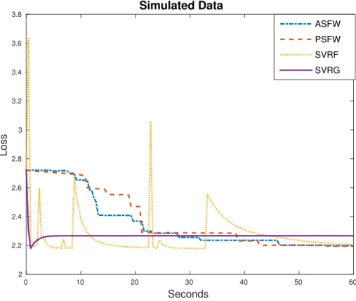
function values obtained by using ASFW, PSFW and Prox-SVRG and the running minimum values obtained by SVRF are plotted against CPU time. From the plot, we can see that ASFW and PSFW performed as well as or slightly better than their stochastic competitors. At the very beginning, both Prox-SVRG and SVRF descents rapidly, while ASFW and PSFW obtains lower function values later on. We also observe big swings in SVRF periodically. This is because at the beginning of each epoch, SVRF proceeds with noisy gradients and very large step sizes. According to Theorem 1 in [30], the step size of the first step in every epoch can be as large as1.

Seconds 0 10 20 30 40 50 60 Loss 2 2.2 2.4 2.6 2.8 3 3.2 3.4 3.6 3.8 Simulated Data ASFW PSFW SVRF SVRG

(45)

3.7.2 Million Song Dataset

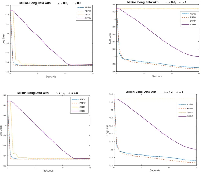
We implemented ASFW and PSFW for solving least squares problems with elastic-net regu-larization and tested them on the Million Song Dataset (YearPredictionMSD) [36][37], which is a dataset of songs with the goal of predicting the release year of a song from its audio features. There are n = 463,715 training samples and p = 90 features in this dataset. The dataset is the one with largest number of training samples available in the UCI machine learning data repository. Therefore it is interesting to examine the actual performance of stochastic algorithms on such a massive dataset. The least squares with elastic-net regularization model that we used was,

min x∈Rp 1 nkAx−bk 2 2+λkxk1+ µkxk 2 2

where A ∈ _Rn×p and b ∈ _Rn. µ ≥ 0and λ ≥ 0are regularization parameters. In the numerical experiments, we considered the constrained version of the problem, that is,

minimize 1 nkAx−bk 2 2+ µkxk 2 2 subject to kxk₁≤ α

whereα >0is inversely related toλ.

We also compared the ASFW and PSFW with SVRF and Prox-SVRG. We followed the same settings in this real data experiment as that in the simulated data experiment except that we used explicit solutions for solving linear optimizations over an l₁-balls in FW algorithms and we used the algorithm in [38] for the solving projections ontol1-balls in the Prox-SVRG algorithm instead of using GUROBI for solving linear optimizations and projections. To make fair comparisons, we used the same starting point for all four algorithms. The logarithm of the loss function values obtained by ASFW, PSFW and Prox-SVRG and the running minimum value obtained by SVRF are plotted against CPU time. The figures indicate that the performance of ASFW and PFW was as good as or better than Prox-SVRG and SVRF under different regularization parameter settings.

(46)

t Seconds 0 5 10 15 Log Loss 13.2 13.4 13.6 13.8 14 14.2 14.4

14.6 Million Song Data with µ = 0.5, α = 0.5

ASFW PSFW SVRF SVRG Seconds 0 5 10 15 Log Loss 12.6 12.8 13 13.2 13.4 13.6 13.8 14 14.2

14.4 Million Song Data with µ = 0.5, α = 5

ASFW PSFW SVRF SVRG Seconds 0 5 10 15 Log Loss 13.2 13.4 13.6 13.8 14 14.2 14.4

14.6 Million Song Data with µ = 10, α = 0.5 ASFW PSFW SVRF SVRG Seconds 0 5 10 15 Log Loss 12.6 12.8 13 13.2 13.4 13.6 13.8 14 14.2

14.4 Million Song Data with µ = 10, α = 5

ASFW PSFW SVRF SVRG

Figure 3.2: Comparisons between algorithms on million song dataset.

We also observed huge swings in SVRF periodically in these experiments. Therefore, we plot the running minimums instead of the most recent function values for SVRF.

3.8 Conclusion and Future Work

In this chapter, we proved linear convergence almost surely and in expectation of the Away-step Stochastic Frank-Wolfe algorithm and the Pairwise Stochastic Frank-Wolfe algorithm by us-ing a novel proof technique. We tested these algorithms by trainus-ing a least squares model with elastic-net regularization on the million song dataset and on a synthetic problem. The proposed al-gorithms performed as well as or better than their stochastic competitors for various choices of the

(47)

regularization parameters. Future work includes extending the proposed algorithms to problems with block-coordinate structures and non-strongly convex objective functions and using variance reduced stochastic gradients to reduce the number of stochastic gradient oracle calls.

(48)

Chapter 4: Local Curvature Based Adaptive Step-size Algorithms

4.1 Introduction

We are concerned with minimizing functions of the form

min

x∈Rn

F(x) =Eξf(x, ξ). (4.1)

Many common problems in statistics and machine learning can be put into this form. For instance, in the empirical risk minimization framework, a model is learned from a set{y1, . . . ,ym} of training data by minimizing an empirical loss function of the form

min x L(x) = 1 m m X i=1 f(x,yi). (4.2)

It is easy to see that this formulation is equivalent to taking ξto be the uniform distribution on the points{y1, . . . ,ym}.

An objective function of the form (4.1) is often impractical, as the distribution of ξ is gener-ally unavailable, making it infeasible to analyticgener-ally compute Ef(x, ξ). This can be resolved by

replacing the expectationEf(x, ξ) by the estimate (4.2). The strong law of large numbers implies

that the sample meanL(x) converges almost surely toF(x) as the number of samplesmincreases, provided that the samples yi are drawn independently from the distribution of ξ. However, even the concrete problem (4.2) is not a good target for classical optimization algorithms, as the amount of datamis frequently extremely large. Thus, a better strategy when optimizing (4.2) is to consider subsamplesof the data to reduce the computational cost. This leads tostochastic algorithmswhere the objective function changes at each iteration by randomly selecting subsamples.

(49)

no-tablystochastic gradient descent(SGD), and variance-reduced extensions of SGD, such as SVRG [6], SAG [7], and SAGA [8]. These methods arefirst-ordermethods, extending gradient descent to the stochastic setting, and the latter three (variance-reduced) methods can be shown to converge linearly for strongly convex objectives. Linearly convergent stochastic Limited Memory BFGS algorithms [39][40] have also been proposed. It is then natural to consider stochastic extensions of quasi-Newton and second-order methods. One such method, the Newton Incremental Method (NIM) [9], combines cyclic updating of a fixed collection of functions f(x,y1), . . . , f(x,ym) with Newton’s method, and attains local superlinear convergence.

One of the key obstacles to developing stochastic extensions of quasi-Newton methods is the necessity of selecting appropriatestep sizes. The analysis of the global convergence of the BFGS method [10] and other members ofBroyden’s convex class[11] assumes that Armijo-Wolfe inexact line search is used. This is rather undesirable for a stochastic algorithm, as line search is both computationally expensive and difficult to analyze in a probabilistic setting. However, there is a special class of functions, the self-concordant functions, whose properties allow us to compute an adaptive step size and thereby avoid performing line searches. In [12], it is shown that the BFGS [13][14][15][16] method with adaptive step sizes converges superlinearly when applied to self-concordant functions.

In this chapter, our goal is to develop a stochastic quasi-Newton algorithm for self-concordant functions. We propose an iterative method of the following form. At the k-th iteration, we draw mk i.i.d samplesξ1, . . . , ξmk. Define theempirical objective functionat the k-th iteration to be

Fk(x) = 1 mk m_k X i=1 f(x, ξi). (4.3)

LetHk be a positive definite matrix. The next step direction is given by

(50)

and the step size by tk = αk 1+αkδk , where αk = ∇Fk(xk)THk∇Fk(xk) δ2 k and (4.4) δk = q ∇Fk(xk)THk∇2Fk(xk)Hk∇Fk(xk).

The motivation for this step size is described in Section 4.4.

A key feature of these methods is that the step sizetk can be computed analytically, using only local information, and adapts itself to the local curvature. A fixed step size η is typically used in the SGD variants, and this step size must be determined experimentally. The theoretical analysis that has been provided for these methods is of little help in choosing η, as oftenη is constrained to be impractically small, and moreover, is related to unknown constants such as the Lipschitz parameter of the gradient. Furthermore, a fixedη which was effective in one phase may become ineffective as the algorithm progresses, and enters regions of varying curvature.

Our new methods are also capable of solving general problems of the form (4.1). This is in contrast to incremental-type methods such as SAG, SAGA, and NIM, which, because of their stored updating scheme, can only be applied to problems of the form (4.2) with a fixed data set

{y1, . . . ,ym}. This opens up new avenues for the solutions of problems where new data can be sampled as the algorithm progresses, as opposed to having a fixed training set throughout.

By choosing the matrices Hk appropriately, we obtain stochastic extensions of classical meth-ods. In particular, two choices ofHk will be of interest:

1. TakingHk = Iyields the stochastic adaptive gradient descent method (SA-GD).

2. FixingH₀, and then takingHk+1to be the BFGS update ofHk, yields the stochastic adaptive BFGS method (SA-BFGS).

(51)

con-verge R-linearly in expectation to an -optimal solution. The SA-BFGS algorithm can also be shown to converge R-superlinearly to the true optimal solution if the number of samples is in-creased so thatm−_k1converges R-superlinearly to 0.

This chapter is organized as follows. In Section 4.2, we introduce our notation, and the techni-cal assumptions needed for the analysis of our methods. In Section 4.3, we describe the relevant results from stochastic analysis which motivate our algorithms. In Section 4.4, we describe the required theory of self-concordant functions. In Section 4.5, we formally define stochastic adap-tive methods, and prove the convergence results. In Section 4.6, we present preliminary numerical experiments, and conclude with a discussion in Section 4.7.

4.2 Assumptions and Notation

The number of variables is n. We usegk(x) = ∇Fk(x) andGk(x) = ∇2Fk(x) for the gradient and Hessian of the empirical objective function. In the context of a sequence of iterates {xk}∞_k₌₀ generated by an algorithm, we also writegkwith no argument to denotegk(xk), andGkforGk(xk). In the context of BFGS,Hk denotes the approximation to the inverse Hessian, andBk = H_k−1.

The optimal solution of min

x F(x) is denoted x

∗

, and the optimal solution of the empirical problemmin x Fk(x) is denotedx ∗ k. Note that x ∗ k is random.

Unless otherwise specified, the normk · kis the 2-norm, or the operator 2-norm. The Frobenius norm is indicated ask · kF.

We make the following technical assumptions on F(x) and f(x, ξ). We will explain the moti-vation behind these assumptions at the relevant points in the discussion.

Assumptions:

1. There exist constants L ≥ ` > 0 such that for every x ∈ _Rn and every realization of ξ, the Hessian of f with respect tox satisfies