JULIA EHRENM ¨ULLER AND JUANJO RU´E
Abstract. By means of analytic techniques we show that the expected number of spanning
trees in a connected labelled series-parallel graph on nvertices chosen uniformly at random satisfies an estimate of the form
s%−n(1 +o(1)),
wheresand%are computable constants, the values of which are approximatelys≈0.09063 and
%−1 ≈2.08415. We obtain analogue results for subfamilies of series-parallel graphs including
2-connected series-parallel graphs, 2-trees, and series-parallel graphs with fixed excess.
1. Introduction
The study of spanning trees and their enumeration is a central question in graph theory and in combinatorial optimization. It is well known that the number of spanning trees of a given graphG
is an evaluation of its Tutte polynomial (see for instance [7]). A lot of research has been devoted to study estimates of this number when dealing with restricted graph families. For instance, various results have been obtained for regular graphs and for graphs with degree constraints (see e.g. [1, 29, 30, 31]).
The enumeration of graphs with a distinguished spanning tree has also been studied extensively in the context of planar maps (namely, embedded connected planar graphs in the sphere, see Schaeffer’s Chapter at [10] for an introduction to this area). The first result in this context was obtained in the sixties by Mullin who was studying the number of rooted planar maps onnedges with a distinguished spanning tree [33]. Mullin determined that this number is CnCn+1, where
Cn stands for the n-th Catalan number. Such formula was explained later by Cori, Dulucq and
Viennot by means of Baxter permutations [15], and by Bernardi using a direct bijection with pairs of plane trees withnandn+ 1 edges, respectively (see [3]). Recently, Bousquet-M´elou and Courtiel investigated the enumeration of regular planar maps carrying a distinguished spanning forest, as well as the connections of these counting formulas with statistical models as the Potts model [11] (see also [4] for the connection of spanning trees on maps and the Tutte polynomial).
In this paper we study spanning trees in series-parallel graphs. A graph is series-parallel (or SP for short) if it is K4-minor free. Over the past few decades, SP graphs have been extensively
studied from various points of view both in graph theory and computer science. In particular, being a subclass of planar graphs and a superclass of outerplanar graphs, SP graphs turned out to serve well as a pre-stage for the analysis and study of problems on planar graphs. Indeed, the family of SP graphs is the prototype of the so-calledsubcritical graph class family (see e.g. [21, 25]). In a typical connected graph in such a family, maximal 2-connected subgraphs (also calledblocks) are small compared with the total size of the graph. This behaviour arises as a consequence of a subcritical composition phenomenon which appears in the specification of the generating functions associated with connected graphs of the family.
In this paper we focus on enumerative problems defined on SP graphs. To this purpose, let us quickly state the following alternative definition of SP graphs that gives more insight into their structure and also justifies their name. LetGbe a graph and letsandtbe two of its vertices. We sayGis series-parallel with terminals sand tifG can be turned into the single edge{s, t} by a
2010 Mathematics Subject Classification: Primary 05A16, Secondary 05C10.
A preliminary version of the results of this paper was presented at theBordeaux Graph Workshopheld in Bordeaux in November 2014. J. R. was partially supported by the FP7-PEOPLE-2013-CIG project CountGraph (ref. 630749), the Spanish MICINN projects MTM2014-54745-P and MTM2014-56350-P, the DFG within the Research Training GroupMethods for Discrete Structures(ref. GRK1408), and theBerlin Mathematical School.
sequence of the following operations: replacement of a pair of parallel edges (i.e. edges that have two common endpoints) by a single edge, or replacement of a pair ofseries edges (i.e. non-parallel edges that have a common endpoint of degree 2) by a single edge. A graphGis2-terminal series-parallel if there are verticess and t in G such that G is series-parallel with terminalss and t. Finally, a graphGis series-parallel if and only if each of its 2-connected components is a 2-terminal series-parallel graph (see e.g. [12]).
Also, SP graphs are known to be the class of graphs of treewidth at most 2 (see e.g. [12]). Edge-maximal SP graphs (i.e. graphs which cease to be SP whenever any missing edge is added) are exactly the class of 2-trees, which can be defined in the following way. A single edge is a 2-tree. IfT is not a single edge, thenT is a 2-tree if and only if there exists a vertexvof degree 2 such that its neighbours are adjacent and T −v is also a 2-tree. Conversely, every subgraph of a 2-tree is a SP graph. In particular, SP graphs are at most 2-connected since 2-connected SP graphs always contain a vertex of degree 2.
From now on, unless stated otherwise, all graphs under study are labelled and simple. By a random object of a given family we mean an object chosen uniformly at random from all the elements of the same size, e.g. graphs on the same number of vertices. In the present paper we study enumerative properties of spanning trees and spanning forests on random SP graphs. Before stating our results, let us survey some relevant related investigations.
One can easily verify that the number of edges of ann-vertex 2-tree is precisely 2n−3. In the same context, Moon [32] showed that the number of 2-trees onnvertices is equal to n2
(2n−3)n−4.
The enumeration of SP graphs is, however, more involved. Bodirsky, Gim´enez, Kang, and Noy proved in [8] that the number of connected SP graphs onnvertices is asymptotically of the form
csn−5/2%−snn!,
where cs≈0.00679 and%s≈0.11021 are computable constants. In the same paper they showed
that the number of edges in a random connected SP graph is asymptotically normally distributed with mean asymptotically equal toκnand variance asymptotically equal toλn, whereκ≈1.61673 andλ≈0.2112 are again computable constants.
Building on these results, a lot of research has been done to understand the qualitative picture that emerges when studying a random SP graph with a fixed number of vertices. The maximum degree and the degree sequence of a random SP graph have been studied in [20] and [6, 19], respectively. Drmota and Noy [21] investigated several extremal parameters in subcritical graph classes, which include the class of SP graphs. They showed, for instance, that the expected diameterDn of a random connected SP graph onnvertices satisfies c1√n≤E[Dn]≤c2√nlogn
for some positive integers c1 and c2. The precise asymptotic estimate has been proved very
recently by Panagiotou, Stufler, and Weller [36] to be of order Θ(√n). In the same work, the authors exploited this fact to prove that in subcritical graph classes, and in particular in SP graphs, the normalized metric space (V(G), dG/√n) (where dG(u, v) is the number of edges in a
shortest path that containsuandv inG) converges with respect to the Gromov-Hausdorff metric to theBrownian Continuum Random Tree multiplied by a constant scaling factor that depends on the class under study (see [36]).
Our results. In the present paper we study the number of spanning trees in a random (connected or 2-connected) SP graph onnvertices. In particular, our main result is a precise estimate of the expected number of spanning trees.
Theorem 1.1. Let Xn and Zn denote the number of spanning trees in a connected, respectively
2-connected, labelled SP graph onnvertices chosen uniformly at random. Then, E[Xn] = s%−n(1 +o(1)), wheres≈0.09063, %−1≈2.08415,
E[Zn] = p$−n(1 +o(1)), wherep≈0.25975, $−1≈2.25829.
The previous analysis is done overall(connected, 2-connected) SP on a given number of vertices. However, we also address the study of extremal situations. First, we can also particularize the computation of the expectation in the case of a random 2-tree on n vertices, which maximizes
the number of edges in ann-vertex SP graph. In this case, the expected value of the number of spanning trees is slightly bigger than the one in Theorem 1.1.
Theorem 1.2. Let Un denote the number of spanning trees in a labelled 2-tree on n vertices
chosen uniformly at random. Then, the expected value of Un is asymptotically equal to s2%−2n,
wheres2≈0.14307 and%−21≈2.55561.
Finally, we study SP graphs with few edges. More precisely, we elaborate the expected number of spanning trees in a random connected SP graph onnvertices andfixed excessequal tok, where
k is a integer that does not depend onn. Recall that the excess of a graph G is defined as the number of its edges minus the number of its vertices (by fixed we mean that it does not grow as a function ofn). Our result is a polynomial estimate (inn) of the expected number of spanning trees:
Theorem 1.3. Let k >1 be a fixed integer. Let Xn,k denote the number of spanning trees in a
connected labelled SP graph, on n vertices and with fixed excess equal to k, chosen uniformly at random.
Then, when nis large enough, E[Xn,k] = ˜c(k) Γ(3k/2) Γ(2k+ 1/2) n 2 k+12 (1 +o(1)),
where the function ˜c(k) satisfies that, forklarge ˜
c(k) = ˜cγ˜−k(1 +o(1)), (1) withc˜≈0.90959 andγ˜−1
≈2.60560.
The previous formulas must be understood in the following way: we fix k and we let ntend to infinity. Additionally, ifk is sufficiently large, we can get the approximation of ˜c(k) stated in the second part of Theorem 1.3. Indeed, the termo(1) in Equation (1) is polynomially small ink
(O(k−1)).
In order to deduce these expressions in Theorem 1.3 we analyse weighted cubic SP multigraphs on 2k vertices. These objects are reminiscent of the work [28] and are building on previous enumerative results on simple cubic planar graphs [9], see Section 6 for definitions and details. The asymptotic estimate stated in Theorem 1.3 arises when getting asymptotic estimates (in terms ofk) for the number of such multigraphs.
Organisation. The rest of the paper is organised as follows. In Section 2 we introduce the essential combinatorial and in Section 3 the essential analytic definitions, techniques, and results that we use. The proof of Theorem 1.1 is then presented in Subsection 4.1 of Section 4. In the same section we also analyse the behaviour of the growth constant of the expected number of spanning trees in a random connected SP graph if we fix its edge density (Subsection 4.2) and comment on the variance of the number of spanning trees in a random 2-connected SP graph (Subsection 4.3). Next, Section 5 is devoted to the analysis of 2-trees and the proof of Theorem 1.2. Then, Section 6 deals with SP graphs with fixed excess and presents the proof of Theorem 1.3. Finally, Section 7 contains some concluding remarks and open problems.
2. Combinatorial Preliminaries
Notation. Our combinatorial and analytic notation is standard and follows [23]. In particular, given a formal power series of exponential typeA(x) =P
n≥0an
xn
n! (EGF for short), we use the
notation [xn]A(x) to indicate the n-th coefficient of A(x). Given a bivariate function A(x, y),
we denote the partial derivative of A(x, y) with respect to x and y by Ax(x, y) and Ay(x, y),
respectively. However, we will usually use the notation A0(x, y) to denote A
x(x, y). We write an ∼bn whenever limn→∞an/bn = 1. Throughout the paper log denotes the natural logarithm.
In our setting, we use the variable x to mark vertices and the variable y to mark edges. These variables are exponential and ordinary, respectively.
Graph decompositions. The main ingredients in our proofs, from an enumerative combinatorial point of view, are the Symbolic Method, generating functions, connectivity decompositions, and an extension of the Dissymmetry Theorem to tree-decomposable classes. In this section we review the essential definitions and results related to these topics. For further details, in particular for an introduction to the Symbolic Method, we refer to the book Analytic Combinatorics by Flajolet and Sedgewick [23].
Let C be a class of connected graphs with the property that a graph is in C if and only if all its 2-connected and 3-connected components are in C. Observe that for instance the class of connected SP graphs carrying a distinguished spanning tree shares this property. Letcn,mdenote
the number of graphs in C with n vertices and m edges. The associated (mixed) exponential generating function (or EGF for short) is the formal power series
C(x, y) = X m,n≥0 cn,m xn n!y m,
wherexandy mark vertices and edges, respectively.
Similarly, letbn,mdenote the number of 2-connected graphs inC withn vertices andm edges
and letB(x, y) be its associated EGF. A connected graph rooted at a vertex can be obtained from a set of rooted 2-connected graphs, where the root is not labelled and where every other vertex is substituted by a connected graph rooted at a vertex. Using the Symbolic Method, this translates into the following relation betweenC(x, y) andB(x, y) (see also [24]).
xC0(x, y) =xexp (B0(xC0(x, y), y)). (2) Following [40], a network is defined as a simple graph with two distinguished vertices, that are called 0-pole and∞-pole and do not bear a label, such that adding an edge between the two poles creates a 2-connected multigraph. If there is an edge joining the two poles, it is calledroot edge. The root edge defines the two poles, which are usually denoted by 0 and∞(initial and final vertex of the root edge, respectively). LetD(x, y) denote the EGF associated with networks. The following equation, shown by Walsh in [40], reflects the relation betweenB(x, y) andD(x, y).
2(1 +y)By(x, y) =x2(D(x, y) + 1). (3)
The left-hand side in Equation (3) corresponds to the family 2-connected graph rooted at a directed edge that might not be present in the graph and the right-hand side corresponds to the family of networks (possibly empty) where in addition a label is given to the two poles.
A trivial network consists of the two poles and of the root edge. Following the ideas of [38], we further distinguish between three types of networks, namely series, parallel, andh-networks as follows. A series networkS can be obtained from a directed cycle with a distinguished edge (which defines the two poles of the network) by replacing every other edge by a network, and finally removing the distinguished edge. A parallel network P arises from merging at least two non-trivial networks, the root edge of each of them being not present, at their common poles. In this family, the root edge joining the two poles of P might not be present inP. Finally, an
h-network is obtained from a 3-connected graphH rooted at an oriented edge, by replacing every edge ofHapart from the root edge by a network. As in the parallel case, here the root edge might not be in the network.
Trakhtenbrot [38] showed that a network is either trivial, series, parallel, or anh-network, and Walsh [40] translated this decomposition into counting formulas. In SP graphs, the set of h -networks is empty, so in the rest of the paper we deal only deal with series and parallel -networks. Let us finally mention that our definition of network slightly differs from Trakhtenbrot’s. Indeed, in [38] series networks could contain the root edge. In our work, series networks containing the root edge (in Trakhtenbrot’s sense) are always considered to be parallel. This convention would arise to be helpful when dealing with spanning trees.
In Section 4 we aim for a precise asymptotic estimate for the number of spanning trees in random SP graphs. For this purpose, we will enumerate the class of connected SP graphs with a distinguished spanning tree. The main idea is to give a complete analytic analysis of the gener-ating function associated with this class using the relations to the class of 2-connected SP graphs
and to the class of networks, both carrying a distinguished spanning tree. Using Equation (3) would imply integration steps that are known to get difficult when considering enriched classes of graphs. Chapuy, Fusy, Kang, and Shoilekova [14] found, however, a convenient combinatorial trick to forgo this integration step by using the dissymmetry theorem for tree-decomposable classes (Theorem 2.1) and by using the grammar for decomposing graphs into 3-connected components that they developed in [14]. Theorem 2.1 will also serve us well in Section 5.
A class A of graphs is tree-decomposable if for each graph G ∈ A we can define a tree τ(G) associated withG. LetA◦denote the class of graphsGinAwhereτ(G) has a distinguished vertex. Similarly, denote byA◦−◦the class of all graphs Gin Awhereτ(G) carries a distinguished edge. Finally, let A◦→◦ be the class of all graphs G in A where an edge of τ(G) is directed. The Dissymmetry Theorem for trees by Bergeron [2] allows to express the class of unrooted trees in terms of classes of trees with a distinguished vertex, edge or with a directed edge. This theorem can be extended to tree-decomposable classes in the following way (see e.g. [14]).
Theorem 2.1 (Dissymmetry Theorem for tree-decomposable classes). Let Abe a tree-decompo-sable class of graphs. Then,
A+A◦→◦' A◦+A◦−◦.
Finally, let us briefly summarize Tutte’s decomposition [39] for decomposing 2-connected graphs into 3-connected components. For a thorough exposition we refer to [14].
Tutte’s decomposition is based on split operations and the structure obtained from this process is shown to be independent of the order of the operations. Roughly speaking, in every split operation we split the edge set of a graphG into two edge setsE1 and E2 that only coincide in
exactly two vertices, sayuandv, and whereG[E1] is 2-connected andG[E2] is connected modulo
{u, v} (meaning that there exists no partition ofE2into two nonempty setsE20 andE200 such that
G[E20] andG[E200] only intersect inuandv). Next we add a so-called virtual edgeebetween these
two vertices. Then we split the graph along this virtual edge which yields two graphsG1 andG2
that correspond respectively toG[E1] andG[E2] withe now being a real edge. We say thatG1
andG2arematched by the virtual edgee.
The resulted structure is a collection of graphs that we call bricks. Tutte showed that there are only three types of bricks, namely ring graphs (R-bricks), multi-edge graphs (M-bricks), and 3-connected graphs with at least 4 vertices (T-bricks). The class of ring graphs is defined as the class of cyclic chains of at least 3 edges and the class of multi-edge graphs as the class of graphs with exactly two labelled vertices that are connected by at least 3 edges.
TheRMT-tree of a graphGis defined as the graph τ(G) the vertices of which are the bricks that result from Tutte’s decomposition applied to G. Two vertices inτ(G) are connected, when the corresponding bricks are matched by a virtual edge. It was shown by Tutte [39] thatτ(G) is indeed a tree and there are no two adjacentR-bricks nor two adjacentM-bricks.
LetBbe the class of all 2-connected graphs with at least 3 vertices. We denote byBR,BM, and BT the classes of graphsGinBsuch that the RMT-tree associated withGcarries a distinguished
R-vertex, M-vertex, and T-vertex, respectively. Moreover, letBR−M denote the class of graphsG
inBsuch that an edge between an R-vertex and an M-vertex in the RMT-tree associated withG
is distinguished. The classesBR−T,BM−T, andBT−T are defined analogously. Finally, letBT→T
be the class of graphsGin Bsuch that an edge between twoT-vertices is directed. Using Theorem 2.1,B satisfies the following equation as shown in [14]:
B ' BR+BM +BT − BR−M− BR−T − BM−T − BT→T +BT−T. (4)
In our work we consider only SP graphs. In particular, a SP graph does not have 3-connected components. This implies that SP graphs do not contain T-bricks, and in hence RMT-trees do not have T-vertices. So Equation (4) is simplified to
B ' BR+BM− BR−M. (5)
3. Analytic Background
The proofs in this paper are based on singularity analysis of generating functions. In this section we introduce the necessary analytic background. For the sake of completeness, we state the
results that we use, in particular a simplified version of the Transfer Theorems (Theorem 3.1) and a simplified version for the singularity analysis of systems of functional equations (Theorem 3.2). For more details, we refer to the books Analytic Combinatorics by Flajolet and Sedgewick [23] andRandom Trees by Drmota [17].
Given a univariate exponential generating function
A(x) =X
n≥0
an xn
n!
we would like to determine an asymptotic estimate of the sequence (an)n≥0. Pringsheim’s Theorem
(see e.g. [23]) assures that generating functions with radius of convergence % and non-negative Taylor coefficients have a singularity at%, in particular a positive real dominant singularity. As shown in [23] (Theorem IV.7), the exponential growth of the sequence (an)n≥0is therefore dictated
by the smallest positive singularity%ofA(x) in the sense that [xn]A(x)
∼Θ(n)%−n,
where Θ(n) grows subexponentially, i.e. lim supn→∞|Θ(n)|1/n = 1. The subexponential term Θ(n) results from the nature of this singularity. The so-calledTransfer Theorems, developed by Flajolet and Odlyzko [22], provide us a convenient way to determine the subexponential term of [xn]A(x). In particular, Theorem 3.1 is a special case of the Transfer Theorems in [23]. For this,
we need the definition of dented domains. Given R, ζ > 0 with R > ζ and 0 < φ < π/2, the domain dented atζ (which we write as ∆ζ(φ, R)) is defined as
∆ζ(φ, R) ={z∈C:|z|< R, z6=ζ,|Arg(z−ζ)|> φ}.
Theorem 3.1. Let α ∈ R\Z− and let A(x) be analytic in a domain ∆%(φ, R) dented at the
smallest positive singularity%of A(x). If, as x→%in∆%(φ, R), A(x)∼c 1−x % −α , then [xn]A(x) = c Γ(α)n α−1%−n(1 +o(1)),
whereΓ(x)is the classical Euler Gamma function defined asΓ(x) =R∞ 0 t
x−1e−tdt.
In this paper, the singular expansion of a generating function A(x) in a domain dented at a singularity%is always of the form
A(x) =A0+A1X+A2X2+. . .+A2k+1X2k+1+O(X2k+2),
whereX =p
1−x/%. The even powers ofX, being analytic functions, do not contribute to the asymptotic of [xn]f(x).
IfA1=A3=· · ·=A2k−1= 0 andA2k+16= 0, then the number (2k+ 1)/2 is called thesingular
exponent. Then, by Theorem 3.1 we get that
[xn]A(x)∼Γ(cα)nα−1%−n
withc=A2k+1andα=−(2k+1)/2. WhenA16= 0 we say thatA(x) has a square-root expansion.
Let us now turn to the asymptotic analysis of systems of functional equations. The main refer-ence for this topic is the paper [16]. We include here a shortened version (see Section 2.2.5. in [17] for the more general statement). Assume thaty1(x), . . . , yk(x) are generating functions satisfying
a functional system of equations. We definey= (y1(x), . . . , yk(x)), and the system satisfied byy
is denoted byy=F(x;y), whereF= (F1, . . . , Fk) is a vector of functions. Thedependency graph G= (V, E) associated with the systemy=F(x;y) is an oriented graph the vertex set of which is
V ={y1, . . . , yk} and−−→yiyj is inE if and only if ∂F∂yji 6= 0. The latter condition indicates that there
is a real dependence between Fi andyj. A dependency graph is said to bestrongly connected if
every pair of vertices can be linked by a directed path. Using this terminology, we can finally state the following result:
Theorem 3.2(Systems of functional equations [17], simplified version). Consider the functional system of equations y = F(x;y) satisfying that each yi is analytic at x = 0. Additionally, we
require that each component of F is an entire function with positive Taylor coefficients, that it is not linear in the components yi and depends on x. Finally, we assume that F(0;y) = 0 and
F(x;0)6= 0. Assume also that the associated dependency graph is strongly connected. Denote by Ik the k×kidentity matrix and by Jac(F)the Jacobian matrix associated withFand with respect
to variablesy1, . . . , yk. Assume that the system of equations
y=F(x;y), 0 = det (Ik−Jac(F))
has a unique solution(x0,y0)in the region of analyticity of each component ofF. Then there is a
unique solutionyof the initial system of equations such that the components ofyhave non-negative Taylor coefficients and a square-root expansion in a domain dented atx=x0.
In order to obtain asymptotic estimates we need to assure that the dominant singularity is unique in a dented domain. This condition is usually satisfied whenever the counting formula
A(x) under consideration cannot be written in the formA(x) =xkf(xr) for non-negative values k ≥ 0 and r ≥ 2. More precisely, we say that a generating function A(x) is aperiodic if there exists a non-negative integer n0 such that [xn]A(x)>0 for n ≥n0. Observe that checking the
aperiodicity condition is straightforward whenever we know that for each number of vertices there exist graphs in the family under study. The generating functions we consider in the forthcoming section (which are defined by an implicit equation, or by means of Theorem 3.2) will satisfy the aperiodicity condition by obvious combinatorial reasons. This will imply uniqueness of the dominant singularity. See [17] for details.
4. Spanning trees in series-parallel graphs
In this section we present the proofs of Theorem 1.1 determining a precise asymptotic estimate for the expected number of spanning trees in random connected SP graphs. Additionally, we elaborate the expected number of spanning trees in a random 2-connected SP graph of a given edge density. Recall that all graphs in this paper are considered to be labelled. In order to count spanning trees in SP graphs, we are concerned with the enumeration of SP graphs carrying a distinguished spanning tree. For this, let cn,m andbn,m now denote the number of connected,
respectively 2-connected, SP graphs with a distinguished spanning tree and letC(x, y) andB(x, y) be their associated counting formula, wherexandy mark again vertices and edges, respectively. Furthermore, letDdenote the class of series-parallel networks carrying a distinguished spanning tree and letD(x, y) be its associated generating function.
4.1. Expected number of spanning trees in random SP graphs. The first step in our proof of Theorem 1.1 is the enumeration of SP networks that carry a distinguished spanning tree. For the purpose of counting spanning trees in SP networks, we need to introduce the following auxiliary class. LetD denote the class of SP networks that carry a distinguished spanning forest with two components, each of which contains one of the poles. LetD(x, y) be its associated EGF. Recall that a network is either trivial, series or parallel. By convention, we assume that networks with a root edge are parallel. Therefore, we define the following classes of networks. Let S and S denote the class of series networks that carry a distinguished spanning tree, respectively a distinguished spanning forest with two components each of which contains one of the poles. We denote their associated EGFs by S(x, y) and S(x, y), respectively. Similarly, let P and P
denote the class of parallel networks and which carry a distinguished spanning tree, respectively a distinguished spanning forest with two components, each of which contains one of the poles. Observe that in both families the root edge might be present. Their associated EGFs are denoted by P(x, y) and P(x, y), respectively. For the sake of readability we may omit the parameters whenever they are clear from the context.
We start with elaborating relations betweenD,D,S,S,P, andP in order to obtain a suitable system of equations. One can easily verify that
and
D(x, y) =y+S(x, y) +P(x, y). (7) Note that in Equation (6) the variabley on the right-hand side corresponds to a trivial network with a distinguished spanning tree, whereas in Equation (7) it corresponds to a trivial network with a distinguished spanning forest that consists of two components of size 1.
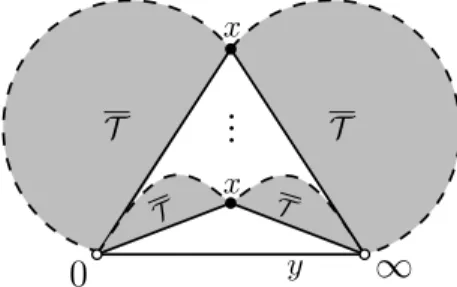
Let us now analyse series networks. Observe that a series networkN can be decomposed into at least two networks, where the 0-pole of the i-th network is identified with the ∞-pole of the (i+ 1)-th network. Equivalently, N can be decomposed into an ordered sequence formed by a networkN0 that is not series and an arbitrary networkN00that are joined by a series operation. IfN ∈ S, then each of these two networks contains a distinguished spanning tree. Therefore, we have S(x, y) = D(x, y)−S(x, y) xD(x, y) = y+P(x, y) xD(x, y). (8)
0
∞
D \ S D Figure 1. Decomposition ofN ∈ S.IfN ∈ S, then eitherN0 ∈ D\S andN00∈ D, orN0 ∈ D\S andN00∈ D. This translates into the following equation:
S(x, y) = D(x, y)−S(x, y) xD(x, y) + D(x, y)−S(x, y) xD(x, y) = y+P(x, y) xD(x, y) + y+P(x, y) xD(x, y). (9)
0
∞
¯ D \S¯ D0
∞
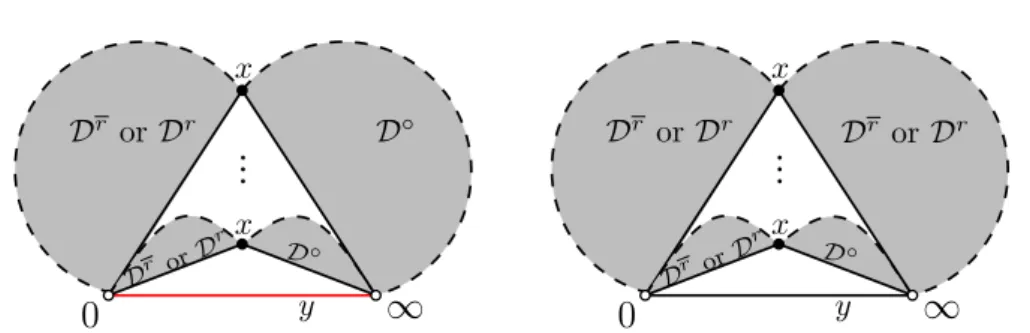
D \ S D¯ Figure 2. Decomposition ofN ∈ S.Finally, we analyse parallel networks. A parallel network can be described as a set of at least one series network if the root edge is present, or of at least two series networks, otherwise. If
N ∈ P, we need to distinguish between the case that the root edge is present and the case that it is not. In the second case, all series networks are in S except for one which is in S. If in the first case the root edge is in the distinguished spanning tree ofN, then all series networks are in
S. If, on the other hand, the root edge is not in the spanning tree, then exactly one of the series networks is inS and all other networks are inS. Thus, we get
P(x, y) =y exp(S(x, y))−1
+y S(x, y) exp(S(x, y))
+S exp(S(x, y))−1
. (10) IfN ∈ P, thenN can be decomposed into the root edge if present and into series networks inS that are joined by a parallel operation. If the root edge is present, then there is at least one other network. In the other case, there must be at least two. This gives rise to the following equation:
P(x, y) = exp(S(x, y))−S(x, y)−1
+y exp(S(x, y))−1
. (11)
Using formal manipulations, we get that the system of Equations (6)-(11) defines the following implicit expression forD(x, y):
D= y+ (1 +y) xD 2 1 +xD exp −xD (y(1 +xD)−(1 +y)D)(2 +xD) (y(1 +xD) + (1 +y)xD2)(1 +xD)2 . (12)
In order to study the singular behaviour of all the previous generating functions we could apply Dromta-Lalley-Woods methodology for systems of functional equations (see e.g. [23]). However,
0 ∞ S y 0 ∞ S S y 0 ∞ S S Figure 3. Decomposition ofN ∈ P. ∞ 0 S ∞ 0 S y Figure 4. Decomposition ofN ∈ P.
as in this particular case we have an expression forD(x, y) not depending on any other variables butxandy, we will analyse Equation (12) in order to get the singular behaviour ofD(x, y). The following theorem is reminiscent to Lemma 3.3. in [25]:
Lemma 4.1. Let D(x, y)be the formal power series defined by the equation Φ(x, y;D(x, y)) = 0, where Φ(x, y;z) =z− y+ (1 +y) xz 2 1 +xz exp −xz (y(1 +xz)−(1 +y)z)(2 +xz) (y(1 +xz) + (1 +y)xz2)(1 +xz)2 .
Then, for every choice of y > 0 it holds that D(x, y) has a unique square-root singularity R(y) such thatD(x, y)has a singular expansion of the following form in a domain dented atx=R(y):
D(x, y) =D0(y) +D1(y)X(y) +D2(y)X(y)2+D3(y)X(y)3+O(X(y)4), (13)
where X(y) =p
1−x/R(y). In particular, for y = 1 we have the numerical values x=R(1) =
R≈0.05668,D0(1)≈1.82404 D1(1)≈ −1.52769,D2(1)≈1.34779 andD3(1)≈ −1.25138.
Proof. Fixy > 0. A simple computation shows that Φz(0, y;D(0, y)) = 1>0 and D(0, y) =y.
Hence, by the Implicit Function Theorem,D(x, y) is analytic atx= 0.
We start with showing that D(x, y) has a finite radius of convergence. Denote the singularity of the function D(x, y) byR(y). Observe that [xn]D
∅(x, y)<[xn]D(x, y), where D∅(x, y) is the generating function associated with SP networks without a distinguished spanning tree. As it is shown in [8], the radius of convergence R∅(y) of D∅(x, y) is finite. In particular, 0 < R(y) ≤
R∅(y)<1<∞andD(x, y) ceases to be analytic atx=R(y).
Observe that the only source of singularity forD(x, y) is the condition Φz(R(y), y;D(R(y), y)) =
0, meaning that the singularity arises from a branch point. Let us now justify that we have Φzz(R(y), y;D(R(y), y))6= 0, which would give the claimed square-root expansion. This condition
is enough in order to assure, for each choice ofy, and square-root type singularity. For a contra-diction, let us assume the opposite. Hence, we have a solution (R0, y0, z0) of the following system
of equations:
Observe that Φ(x, y;z) =z−A(x, y;z) exp(B(x, y;z)) withA(x, y;z) andB(x, y;z) being rational functions. Hence, Φz(x, y;z) = 1−C(x, y;z) exp(B(x, y;z)) where again C(x, y;z) is a rational
function. Finally, Φzz(x, y;z) can be written in the form E(x, y;z) exp(B(x, y;z)) for a certain
rational functionE(x, y;z).
In particular, combining the first two equations by eliminating the exponential term, we get the following system of rational equations:
zC(x, y;z) =A(x, y;z), E(x, y;z) = 0.
After rearranging the denominators in both expressions, such a system can be transformed into a system of two polynomial equations P1(x, y;z) = 0, P2(x, y;z) = 0, from which we can get a
new polynomial equationQ(x, y) = 0 by eliminating the variablez. By carrying out the explained computations withMaple, we obtain
Q(x, y) = (−4y+yx−4)y(y+ 1)T(x, y),
where
T(x, y) = 100(1 +y)4+ 6917y(1 +y)3x+ 1266y2(1 +y)2x2
−1867y3(1 +y)x3+ 280y4x4.
We now argue thatQ(x, y) = 0 does not have a solution with bothy >0 andx <1. Observe that the first multiplicative term−4y+yx−4 gives the solution (x, y) = (4 + 4/y, y). This means in particular thatxis always greater than 1. It is also obvious that the multiplicative termsy and
y+ 1 cannot contribute with the required solution. Therefore, we need to analyse the existence of solutions (x, y) ofT(x, y) with the conditiony >0 andx <1. Using thaty(1+y)3> y3(1+y),x >
x3for ally >0 and 0< x <1, we know that 6917y(1 +y)3x >6917y3(1 +y)x3>1867y3(1 +y)x3.
Hence,T(x, y) = 0 does not have solutions with both 0< x <1 andy >0, which implies that the solution (x0, y0, z0) of the equation Φ(x, y;z) = Φz(x, y;z) = 0 satisfies that Φzz(x0, y0;z0)6= 0.
Hence, the singularity ofD(x, y) is of a square-root type in a domain dented atx=R(y). This proves the singular expansion in Equation (13).
In order to prove the special case of y = 1 in the statement of the lemma, we set y = 1,
R=R(1), andX =X(1) (and consequentlyx=R(1−X2)). By plugging the singular expansion
ofD(x,1) in Φ(x, y;z) = 0, taking the Taylor expansion in terms of X, and applying the method of indeterminate coefficients, we get the numerical values as claimed. Finally, observe that for each choice of y > 0, the generating function D(x, y) is aperiodic, as for every n there exists a network onnvertices. This gives that the singularityR(y) is unique, and the result holds.
Knowing that D(x, y) admits a singular expansion of square root-type in a domain dented at x = R(y), one can compute by means of indeterminate coefficients the exact expressions of
Di(y) for i ≥ 1 in terms of the function D(R(y), y) = D0(y), which satisfies the functional
equation Φ(R(y), y, D0(y)) = 0. Although the expressions are long, we need to compute for
enumerative purposes the evaluations at y = 1. For computational purposes, we include the following lemma where the coefficients of the singular expansions (rounded up to 5 digits) of the EGF D(x,1), S(x,1), S(x,1), P(x,1), and P(x,1) are obtained. Despite that in order to get asymptotic estimates for these counting formulas we only need the multiplicative constant of the term (1−x/R)1/2, in order to get the precise asymptotic in the 2-connected level we need
expansions up to term (1−x/R)3/2.
Lemma 4.2. For each value of y > 0 the generating functions D, S, S, P, and P have a square-root singular expansion in a domain dented atR(y), where R(y) is the unique singularity ofD(x, y). Furthermore, fory= 1the singular expansions (with rounded coefficients) ofD,S,S,
P, andP in a domain dented atR≈0.05668 are D(x,1) =D0(1) +D0(1)X+D2(1)X2+D3(1)X3+O(X4) S(x,1) =S0(1) +S1(1)X+S2(1)X2+S3(1)X3+O(X4) S(x,1) =S0(1) +S1(1)X+S2(1)X2+S3(1)X3+O(X4) P(x,1) =P0(1) +P1(1)X+P2(1)X2+P3(1)X3+O(X4) P(x,1) =P0(1) +P1(1)X+P2(1)X2+P3(1)X3+O(X4), whereX =p
1−x/R, and the constants have the following approximate values:
i= 0 i= 1 i= 2 i= 3 Di(1) 1.71871 −1.17120 1.17120 −0.59820 Si(1) 0.17092 −0.27289 0.18433 −0.15440 Si(1) 0.30701 −0.43079 0.19616 −0.12220 Pi(1) 0.65312 −1.25480 1.16347 −1.09697 Pi(1) 0.41170 −0.74041 0.58941 −0.47600
Proof. The first claim follows directly due to Equations (6)-(11), which are analytic and allow us to express D, S, S, P, and P in terms ofD. In particular, all these generating functions have a unique singularity atx=R(y). The second part follows by settingy = 1 and by plugging the singular expansion ofD(x,1) into Equations (6)-(11). Now we turn to the analysis ofB(x, y), the EGF associated with the class of 2-connected SP graphs carrying a distinguished spanning tree. In our context, Equation (3) translates to
2(1 +y)By(x, y) =x2
1 +D(x, y) +D(x, y)−y exp(S(x, y)−1)
(14) which roughly speaking means that when marking an edge in a 2-connected SP graph with a distinguished spanning tree, the resulting object is a network either of type D or D, but not a parallel network of typePwith an edge linking the poles (see Equation (11)). A direct integration of Equation (14) is technically involved due to the relations between the generating functions associated with the different types of networks. However, we can get a simple expression of
B(x, y) in terms of the EGF associated with the networks just by combinatorial arguments. In the following lemma we provide such an equation.
Lemma 4.3. The EGF B(x, y) associated with the class of 2-connected SP graphs carrying a distinguished spanning tree can be expressed as
B(x, y) =x 2 2 y+BR(x, y) +BM(x, y)−BR−M(x, y), (15) where BR(x, y) = x2 2 S(D−S), (16) BM(x, y) =x 2 2 S exp(S)−S−1 +yS exp(S)−1 +y exp(S)−S−1 , (17) BR−M(x, y) = x2 2 (SP+SP). (18)
Proof. Applying Tutte’s decomposition to 2-connected SP graphs bearing a distinguished spanning tree on at least 3 vertices only yields R-bricks (ring graphs) and M-bricks (multi-edge graphs), both carrying a distinguished spanning tree. In particular, there are no T-bricks since the set of
h-networks is empty in our case. We obtain Expression (15) for B(x, y) using Equation (5) to which we needed to addx2y/2 since we also consider a single edge to be a 2-connected SP graph.
Let us study each term. LetR be a distinguished R-brick with a distinguished spanning tree. By definition,Ris a cyclic chain of at least 3 networks that carries a spanning tree. In particular, exactly one of these networks is in D while the other ones are in D. This means that R can be decomposed into a non-series network in D and a series network in S that are joined by a
parallel operation and where the two poles are added to the graph, see also Figure 5. This gives Equation (16).
0
∞ S
D
Figure 5. Decomposition of a distinguished R-brick in the RMT-tree.
We continue with M-bricks. LetM be a distinguished M-brick with a distinguished spanning tree. Then,M can be decomposed into at least three networks, all but possibly one of which are series and the possibly other one a single edge. These networks are joined by a parallel operation and the two poles are again added to the graph. This situation is similar to the decomposition of parallel networks carrying a spanning tree that we considered for developing Equation (10). The main difference is that, by definition, M is decomposed into at least three and not into at least two networks. We need to distinguish again between the two cases where there is a single edge component in M and where there is no such a component. Observe that it is not possible that there are two such components in M since we are only considering simple graphs. In the former of the two cases, we note that if the edge of the single edge component is contained in the distinguished spanning tree, then exactly one of the series networks is inSwhile all the others are inS. If, on the other hand, the edge is not in the spanning tree, then all series networks must be inS. This gives rise to Equation (17).
Finally, we need to decompose 2-connected SP graphs with a distinguished spanning tree and with a distinguished {R, M}-edge in the RMT-tree. This means, that the distinguished edge corresponds to a virtual edge{x, y} matching a R-brick and a M-brick. Hence the graphs can be decomposed into a series network and a parallel network by a parallel operation, where we need to add again the two poles to the graph. One of the two networks must be inDwhile the other one must be inD. Hence, Equation (18) holds. See Figure 6 for an illustration of this situation.
0 ∞ S P 0 ∞ S P
Figure 6. Decomposition of a distinguished{R, M}-edge in the RMT-tree. We can now analyse the singular behaviour ofB(x, y).
Lemma 4.4. Let y >0. Then, B(x, y) has a unique square-root singularity, which is the unique singularityR(y)of the functionD(x, y)in Lemma 4.1. Moreover,B(x, y)has a singular expansion of the following form in a domain dented at x=R(y):
B(x, y) =B0(y) +B2(y)X(y)2+B3(y)X(y)3+O(X(y)4), (19)
whereX(y) =p
1−x/R(y). When y= 1we have the numerical valuesx=R(1) =R≈0.05668,
B0(1)≈0.00176,B2(1)≈ −0.00394 andB3(1)≈0.00062.
Proof. Observe that the generating functions BR(x, y), BM(x, y) and BR−M(x, y) are analytic
transformations of the generating functions for networks (namely, the EGFs in Lemma 4.3). Hence,
B(x, y) has a unique dominant singularity which is the same one as the coinciding singularity of EGFs of Lemma 4.2, namely R(y). Similarly, for each y, B(x, y) admits a singular expansion in a domain dented at R(y). In order to obtain it, we express the singular expansion of each of the network exponential generating functions appearing in Equation (15) in terms of the singular expansions obtained in Lemma 4.2. Observe that Equation (14) implies that the singular expansion ofB(x, y) must start atX(y)3, which gives in particular thatB
1(y) = 0 (see Theorem VI.9 from
[23]).
Finally, by setting y = 1 and by the same procedure as above using Maple, we obtain the approximation of Bi(1) for i≥0 as stated in the lemma. In particular, the termB3(1) depends
on all singular coefficients in Lemma 4.2. Finally, we analyse the generating function C(x, y) of connected SP graphs carrying a dis-tinguished spanning tree. Since the singular expansion of B(x, y) is of a square-root type with exponent 1/2 as it is shown in Equation (19), we get the singular expansion ofC(x, y) immediately from Proposition 3.10 in [25] (see also [21]).
Lemma 4.5. The singularity of C(x, y) is at ρ(y) = τ(y)/exp(Bx(τ(y), y)), where τ(y) is the
unique solution of the equation τ(y)Bxx(τ(y), y) = 1. The singular expansion of C(x, y) in a
domain dented atρ(y)is C(x, y) =C0(y) +C2(y)X(y)2+C3(y)X(y)3+O(X(y)4), whereX(y) =p1−x/ρ(y)and C0(y) =τ(1 + logρ(y)−logτ(y)) +B(τ(y), y), C2(y) =−τ(y), and C3(y) = 3 2 s 2ρ(y) exp(Bx(ρ(y), y)) τ Bxxx(τ(y), y)−τ Bxx(τ(y), y)2+ 2Bxx(τ(y), y) .
Additionally, when y = 1we have ρ(1)≈0.05288,C0(1)≈0.05450,C2(1) =−τ ≈ −0.05668,
andC3(1)≈0.00145.
Proof. See the proof of Proposition 3.10 in [25] for the analysis for a general value of y. When
y= 1, we useMapleto obtain the approximations of the constants. The unicity of the singularity is assured by the aperiodicity of C(x, y) with y being fixed. See for instance the proof of [18,
Lemma 7] and [18, Lemma 9].
Now we have all necessary ingredients to prove the main theorem of this section.
Proof of Theorem 1.1. We will prove the statement forXnin detail. The result forZn is obtained
mutatis mutandis. Let us denote byCn the set of all connected SP graphs onnvertices, andCns
the set of all connected SP graphs on n vertices carrying a distinguished spanning tree. For a graph G∈ Cn we write s(G) for the number of spanning trees inG. Then, the expected value of Xn can be written as:
E[Xn] = X G∈Cn s(G)P[G] = P G∈Cns(G) |Cn| = |C s n| |Cn| = [x n]C(x,1) |Cn| . (20)
It follows directly from Lemma 4.5 and Theorem 3.1 that the number of connected SP graphs onn
vertices that carry a distinguished spanning tree is asymptotically equal to C3(1)
Γ(−3/2)n−
5/2ρ(1)−nn!.
The number of connected SP graphs onnvertices is asymptotically equal tocsn−5/2%−snn!, where cs ≈0.0067912 and %s ≈0.11021 are computable constants, as shown in [8, Theorem 3.7].
Di-viding the former by the latter as in Equation (20), we obtain that the expected value ofXn is
asymptotically equal tos%−n, where s
≈0.09063 and %−1
≈2.08415.
The corresponding result for 2-connected SP graphs is obtained analogously by using Theo-rem 2.6 of [8], which states that the number of 2-connected SP graphs onnvertices is asymptoti-cally equal tobn−5/2r−nn!, whereb≈0.00101 andr≈0.12800.
4.2. Fixing the edge density and limiting distributions. The previous results can be used to study random SP graphs with a fixed edge density, as well as limiting distributions for the number of edges. For sake of brevity, we only discuss the family of 2-connected SP graphs, but similar observations hold in the connected case. The first main important observation is that the number of edges in a uniformly at random 2-connected SP graph carrying a distinguished spanning tree follows a normal limiting distribution: Lemma 4.4 shows that the singular behaviour of B(x, y) is the same when choosing y in a real-valued neighbourhood of 1. Then, by the Quasi-Powers Theorem by Hwang (see [26]) the distribution follows a normal limit law with linear expectation and variance. In particular, the number of edges is concentrated around its mean value. This behaviour is similar to the case of 2-connected SP graphs (without a spanning tree), where again the number of edges is normally distributed (see [8]).
Under these circumstances, our techniques also provide a method to study the expected number of spanning trees in a random SP graph on n vertices of a given edge densityµ. Following the arguments of [24, Theorem 3], for every µ > 0 we can choose a value y0 > 0 such that if we
assign the weight yk
0 to each graph withk edges, then only the graphs with nvertices and with
approximatelyµnedges (with a deviation of ordern1/2) have non-negligible weight. Such technique
is valid whenever Quasi-Powers Theorem holds, and hence we can apply it in our context. As a case example, we plot the expected value of the random variable Xn,µ that counts the
number of spanning trees in a graph chosen uniformly at random from the 2-connected SP graphs withnvertices and edge density µ. LetR(y) denote the radius of convergence ofB(x, y). Given an edge densityµ, the right choice fory0 is the unique positive solution of the following equation
(see e.g. [24, Theorem 3]):
−y0
Ry(y0)
R(y0)
=µ. (21)
Observe that when µ tends to 1, the family of SP graphs under study are graphs with a small but positive number of cycles, whereas whenµtends to 2, the subfamily under study tends to the class of 2-trees. These cases correspond to the ones wheny tends to 0 and infinity, respectively. Both cases will be analyzed fully in detail in Sections 5 and 6, respectively.
The precise computational method to obtain the exponential growth constant of the expected value ofXn,µas a function of the edge density is the following. For a given density µwe use (21)
to obtain the correspondingy0. Then we use the implicit expression of the singularity curve stated
in Theorem 2.2. of [8] in order to obtain the growth constant of the number of 2-connected SP graphs of edge density equal to µ. To get the growth constant in the setting of 2-connected SP graphs carrying a spanning tree and with edge density µ, we perform the calculations explained in the proof of Lemma 4.1 fory0. Finally, the exponential growth of the expected value ofXn,µis
obtained by dividing these two numerical values as we did in the proof of Theorem 1.1. In Figure 7 we plot this exponential growth constant in terms of the edge densityµ∈(1.07626,1.97173).
Let us mention that the non-plotted margins forµcorrespond to values ofy very close to 0 and when y tends to infinity. In both cases, the numerical method used to get the constant growth for the number of spanning trees fails because of indetermination of the operation to be carried. Detailed analysis of the two cases when the edge density reaches its maximum and when it tends to its minimum will be carried out in Section 5 and in Section 6, respectively.
Figure 7. Exponential growth constant of the expected number of spanning trees in a random 2-connected SP graph (ordinate) as a function of its edge density (abscissa).
4.3. Variance of the number of spanning trees in random SP graphs. Refining the com-binatorics exploited in the proof of Theorem 1.1, one has also access to the second moment of the random variablesXn andZn. In this subsection we develop this by determining the growth
constant of the variance ofZn. This will also show thatZnis not concentrated around its expected
value. Recall thatZn was defined as the random variable which counts the number of spanning
trees in a random 2-connected SP graph onnvertices.
In order to determine the growth constant of the second moment of Zn, we will first study
the asymptotic behaviour of the number of 2-connected SP graphs on n vertices carrying two distinguished spanning trees. As in Subsection 4.1, we start with the analysis of networks carry-ing spanncarry-ing trees and spanncarry-ing forests. We define D∗, S∗, and P∗ as the classes of SP, series, and parallel networks, respectively, each carrying two distinguished spanning trees. LetD∗(x, y),
S∗(x, y), andP∗(x, y) denote their EGFs. In order to be able to analyse these functions, we need again some auxiliary classes. LetDe denote the class of all SP networks carrying a distinguished
spanning tree and a distinguished spanning forest with (exactly) two components each of which contains one pole. Furthermore, let ˆD denote the class of all SP networks carrying two distin-guished spanning forests both with (exactly) two components each of which contains one pole. LetDe(x, y) and ˆD(x, y) denote their EGFs. In the same waySe, Pe, ˆS, and ˆP as well as Se(x, y),
e
P(x, y), ˆS(x, y), and ˆP(x, y) are defined. We might again omit the parameters whenever they are clear from the context. Following the proof of Theorem 1.1, we start with the following lemma that provides the growth constant of these generating functions.
Lemma 4.6. For y = 1, the generating functions D∗, De, Dˆ, S∗, Se, Sˆ, P∗, Pe, and Pˆ have a square-root expansion in a domain dented atR2≈0.02407.
Proof. We start again with elaborating relations between all given generating functions. One can verify easily that the following relations hold:
D∗(x, y) = y+S∗(x, y) +P∗(x, y),
e
D(x, y) = y+Se(x, y) +Pe(x, y), (22)
ˆ
Recall that a series network can be decomposed into a network that is not series and an arbitrary SP network. Similarly to Equations (8) and (9), we get the following equations for the generating functions associated with the networks from the classesS,Se, and ˆS.
S∗(x, y) = D∗(x, y)−S∗(x, y) xD∗(x, y), e S(x, y) = De(x, y)−Se(x, y) xD∗(x, y) + D∗(x, y)−S∗(x, y) xDe(x, y), (23) ˆ S(x, y) = D∗(x, y)−S∗(x, y) xDˆ(x, y) + ˆD(x, y)−Sˆ(x, y) xD∗(x, y) +2 De(x, y)−Se(x, y) xDe(x, y).
Finally, a parallel network can be decomposed into a set of at least one series network if the root edge is present, or into at least two series networks, otherwise. In the first case we need to distinguish whether the root edge is in a distinguished spanning tree or not. By a careful case distinction, we get the following three equations:
P(x, y) = S(x, y) exp( ˆS(x, y))−1 + (1 +y)Se(x, y)2exp( ˆS(x, y)) +yS(x, y) exp( ˆS(x, y)) +2ySe(x, y) exp( ˆS(x, y)) +y exp( ˆS(x, y)−1 , e P(x, y) = y+Se(x, y) exp( ˆS(x, y))−1 +ySe(x, y) exp( ˆS(x, y)), (24) ˆ P(x, y) = exp( ˆS(x, y))−Sˆ(x, y)−1 +y exp( ˆS(x, y))−1 .
Equations (22)-(24) define a system of functional equations that can be analysed by means of Theorem 3.2 by setting y = 1. More precisely, each equation in this system is defined by an analytic function, because the exponential function is an entire function. In addition, easy lower and upper bounds imply that the radius of convergence of D(x,1),De(x,1),Dˆ(x,1) is in (0, R],
whereR≈0.05668 is the constant obtained in Lemma 4.1. Solving the system of equations stated in Theorem 3.2 using Maple we get thatR2 ≈0.02407. Furthermore, Theorem 3.2 assures that
R2 is the singularity of all generating functions appearing in Equations (22)-(24) and that they
have a square-root expansion in a domain dented atR2. As all generating functions written so far
are aperiodic, the singularity is unique on the circle|x|=R2.
LetB∗(x, y) denote the EGF associated with the class of all 2-connected SP graphs carrying two spanning trees. As in Lemmas 4.3 and 4.4 one can writeB∗(x, y) as an analytic combination of the generating functions from Lemma 4.6 by using Tutte’s decomposition and Equation (5). Therefore, the dominant singularity of B∗(x,1) is the same as the coinciding singularity of the EGFs appearing in Lemma 4.6, which isR2, and moreover,B∗(x,1) has a square-root expansion
in a domain dented atR2. By Theorem 3.1 we get that the number of 2-connected SP graphs on
nvertices carrying two spanning trees is asymptotically equal to Θ n−5/2R−n
2 n!
.
Let Bn denote the number of 2-connected SP graphs on n vertices and SB∗n the number of
2-connected SP graphs onnvertices carrying two spanning trees. The second moment ofZn can
be calculated in the following way: E[Zn2] = X G∈Bn s(G)2 P[G] = |SB ∗ n| |Bn| =[x n]B∗(x,1) |Bn| ,
where again s(G) denotes the number of spanning trees in a graphG. Recall that the number of 2-connected SP graphs on n vertices is asymptotically equal to Θ n−5/2r−nn!
, where r ≈
0.12800. This means that the second moment ofZn is asymptotically equal to Θ $2−n
, where
$2−1 ≈ 5.31718. The same holds for Var(Zn) = E[Z 2
n]−E[Zn]2 since E[Zn] is approximately
equal to Θ (%−n), where%−1
≈2.08415 by Theorem 1.1. In particular, this implies thatZn is not
concentrated around its expected value.
5. Spanning trees in2-trees
In Subsection 4.2 we analysed the exponential growth constant of the expected number of spanning trees in a random 2-connected SP graph with respect to its edge density. Observe that if
the edge density of SP graphs tends to its maximum, we reach the class of 2-trees. In this section we present an alternative, direct way to compute this growth constant in the setting of 2-trees. More precisely, we give a proof of Theorem 1.2, which is again based on the Symbolic Method, the extension of the Dissymmetry Theorem to tree-decomposable classes (Theorem 2.1), and the singularity analysis of generating functions. As in the previous section, we use xand y to mark vertices and edges, respectively. In this particular scenario the number of edges is determined once fixing the number of vertices. However, for pedagogical reasons, we will write all the equations keeping track of both parameters. Recall that all graphs in this paper are considered to be labelled, unless otherwise specified.
In order to obtain the expected number of spanning trees in a random 2-tree, we aim to determine the asymptotic precise estimate of the number of trees as well as of the number of 2-trees carrying a distinguished spanning tree. As a first step, Lemma 5.1 provides the singularity%T
and the singular expansion in a domain dented at%T of the generating functionT(x, y) associated
with the class of 2-trees.
Lemma 5.1. Fory= 1it holds thatT(x, y)has a unique square-root type singularity%T = 1/(2e)
and admits the following singular expansion in a domain dented atx=%T: T(x,1) = 1 12e −3/2 −163 e−3/2X2+ √ 2 48e −3/2X3+ O(X4), whereX =p 1−x/%T.
Proof. LetT denote the class of labelled 2-trees rooted at an edge the endpoints of which do not bear a label and letT(x, y) denote its associated generating function. By the rules of the Symbolic Method for pointing operations we have the following relation betweenT(x, y) andT(x, y):
y ∂
∂yT(x, y) = x2
2 T(x, y).
Observe that we had to add the factor x2/2 on the right-hand side because we had to add labels
to the endpoints of the root edge. By integrating by substitution we get that
T(x, y) = x 2 2 Z y 0 T(x, z) z dz= x2 2 T(x, y)−2 3xT(x, y) 3 .
In order to compute the radius of convergence of T(x, y), it suffices to compute the radius of convergence of T(x, y) since their values coincide by the latter equation. A graph in T can be reconstructed by merging at the root edge a set of pairs of graphs in T that share a vertex, see Figure 8. Using the Symbolic Method this gives rise to the following equation forT(x, y):
T(x, y) =yexp xT(x, y)2.
By Lagrange’s Theorem (see e.g. [23]) we get for everyn, m≥0 that
T T T T
0
y∞
x xFigure 8. Decomposition of rooted 2-trees.
[xn][ym]T(x, y) = [xn]1 m[u m−1]emxu2 = [xn]1 m[u m−1]mm−21xm2−1 = ( 1 (m−1 2 )! mm−23 ifn=m−1 2 0 otherwise.
We study the case y = 1 since the number of edges of a 2-tree is determined by its number of vertices. The inverse function of T(x,1) is given by ψ(u) = log(u)/u2. Let τ > 0 such that
ψ0(τ) = 1−2 log(τ)
/τ3= 0, implyingτ = exp(1/2). Then we know from the Inverse Function
Theorem that we have for the singularity %T of T(x,1) that %T = ψ(τ) = 1/(2e). Therefore, T(x,1) and hence also T(x,1) have a square-root type singular expansion in a domain dented at
%T. By the method of indeterminate coefficients we get that the singular expansion ofT(x,1) is of
the form as stated in the lemma. Finally, by aperiodicity of the generating functions under study, the dominant singularity ofT(x,1) is unique. Now let us turn to 2-trees carrying a spanning tree. We denote this class by Ts and its
associated generating function by Ts(x, y). Similarly to Section 4, we need to first analyse
edge-maximal SP networks to get access to the singular behaviour of Ts(x, y). For this purpose, let Dr(x, y) denote the EGF associated with the set of all edge-maximal SP networks carrying a
spanning tree that contains the root edge. Furthermore, let Dr(x, y) denote the EGF associated
with the set of all edge-maximal SP networks carrying a spanning tree that does not contain the root edge. Finally, let D◦(x, y) denote the EGF associated with the set of all edge-maximal SP networks with a distinguished spanning forest that consists of exactly two components each of which contains one of the poles. Observe that we have Dr(x, y) =D◦(x, y). Lemma 5.2 gives us the singular behaviours ofDr=D◦ andDr fory= 1.
Lemma 5.2. We haveDr=D◦ and fory= 1the generating functionsDrandDrhave the same
unique square-root singularityRT ≈0.07197. Furthermore, the singular expansions (with rounded
coefficients) ofDr(x,1) andDr(x,1) in a domain dented at x=R T are:
Dr(x,1) = 1.46516−0.77028X+ 0.53282X2−0.40927X3+O(X4), Dr(x,1) = 0.34588−0.77028X+ 0.87870X2−0.92279X3+O(X4),
whereX =p
1−x/RT.
Proof. Using the Symbolic Method (see also Figure 9) one can easily verify that the following system of equations hold:
Dr(x, y) =yexp2 Dr(x, y) +Dr(x, y) xDr(x, y), Dr(x, y) =yx Dr(x, y) +Dr(x, y)2 exp2 Dr(x, y) +Dr(x, y) xDr(x, y). (25) Dr orDr Dr orD r D◦ D◦
0
y∞
x x Dr orDr Dr orD r D◦ Dr or Dr0
y∞
x xFigure 9. Possible decompositions of an edge-maximal SP network with a distin-guished spanning tree that contains the root edge (depicted on the left side)/does not contain the root edge (depicted on the right side).
We may set y = 1 since the number of edges of 2-trees is always given by the number of vertices. The two equations in (25) are defined by entire functions. As these structures carry spanning trees, the corresponding singularity is smaller than %T, and hence their singularityRT
is finite. We can apply Theorem 3.2 and know therefore that Dr(x,1) and Dr(x,1) have the
this singularity. Solving the system of equations stated in this theorem with Maple yields that
RT ≈ 0.07197. By aperiodicity of the counting formulas, this is the unique smallest dominant
singularity. By means of indeterminate coefficients we get the exact coefficients of the singular expansions ofDr(x,1) andDr(x,1) which are the ones as stated in the lemma.
Lemma 5.3. Lety= 1. Then,Ts(x,1) has a square-root singularity, which is the singularityR
T
of Dr(x,1) andDr(x,1). Moreover,Ts(x,1)has a singular expansion of the following form in a
domain dented atx=RT ≈0.07197: Ts(x,1) =Ts 0 +T2sX 2+Ts 3X 3+ O(X4), where X = p
1−x/RT and T0s ≈ 0.00290, T2s ≈ −0.00669, and T3s ≈ 0.00133 are computable
constants.
Proof. We define the ∆e-tree τ(G) of a graph Gas the bipartite graph describing the incidences between edges and triangles of G. More precisely, the node set of τ(G) is given by E(G)∪
{x1, x2, x3}:{xi, xj} ∈E(G) for eachi6=j ∈ {1,2,3} and two nodeseand ∆ are neighbours
if and only ife(∆ inG.
Since we are dealing with graphs carrying a spanning tree we need to encode the information on the distinguished spanning tree also in the associated ∆e-tree. For this reason, we define five different types of nodes of τ(G) if G ∈ Ts. Let V
e and Ve denote the set of vertices of τ(G)
associated with edges of Gthat are, respectively are not contained in the distinguished spanning tree of G. Moreover, fori∈ {1,2,3}, let V∆i denote the sets of vertices ofτ(G) associated with triangles ofGwhich contain exactly 3−iedges that are in the distinguished spanning tree.
Observe that for every G ∈ Ts the connected ∆e-tree τ(G) associated with it is uniquely
defined. We claim that τ(G) is a tree. Indeed, assume for a contradiction that there exists a cycle C = ∆1e1∆2. . .∆kek∆1 in τ(G). Let G0 be the induced subgraph of Gon the vertex set S
i∈[k]∆i. In particular, being edge-maximal andK4-minor free,G0 is also a 2-tree. However, G0
does not contain a vertex of degree 2, a contradiction. As a consequence, τ(G) is indeed a tree. This means that Tsis a tree-decomposable class and therefore we can apply Theorem 2.1. Since
∆e-trees are bipartite, the equation in Theorem 2.1 simplifies to Ts ' Ts
◦ − T◦−◦s . The class T◦s is naturally partitioned into the five classesTs
e,Tes,T∆s1,T s
∆2, andT s
∆3 depending on whether the
distinguished node is from the set Ve, Ve, V∆1, V∆2, orV∆3. The class T s ◦−◦ is partitioned into the classes Ts e−∆1, T s e−∆2, T s e−∆1, T s e−∆2, and T s
e−∆3 by the structure ofτ(G). In terms of their
associated generating functions these facts translate into
Ts=Ts e +Tes+T∆s1+T s ∆2+T s ∆3−T s e−∆1−T s e−∆2−T s e−∆1−Te−∆2−T s e−∆3. (26)
Using the Symbolic Method, it is not difficult to check that the following equations are true. Recall that we haveDr(x, y) =D◦(x, y). Ts e(x, y) = x2 2 D r(x, y), Ts e = x2 2 D r(x, y), Ts ∆1(x, y) = x3 2 D r(x, y)3 , T∆s2(x, y) =x 3 Dr(x, y)2 Dr(x, y), T∆s3(x, y) = x3 2 D r(x, y) (Dr(x, y))2 and Tes−∆1(x, y) =x 3 Dr(x, y)3 , Tes−∆2(x, y) =x 3 Dr(x, y)2 Dr(x, y), Ts e−∆1(x, y) = 1 2x 3 Dr(x, y)3 , Ts e−∆2(x, y) = 2x 3 Dr(x, y)2 Dr(x, y), Tes−∆3(x, y) = 3 2x 3Dr(x, y) (Dr(x, y))2 .
In particular, Ts(x, y) can be expressed in terms ofx, Dr(x, y), and Dr(x, y) by plugging the
previous equations in Equation (26). One can therefore easily verify that the dominant singularity of Ts(x,1) is the same as the coinciding one of Dr(x,1) and Dr(x, y), namely R
T. Finally, we
obtain the singular expansion ofTs(x,1) in a domain dented atR
T by using Equation (26) and
the singular expansions ofDr(x,1) andDr(x,1) from Lemma 5.2.
Now we have all ingredients that we need to finally prove Theorem 1.2.