DL-DI: A DEEP LEARNING FRAMEWORK FOR DISTRIBUTED, INCREMENTAL IMAGE
CLASSIFICATION
A THESIS IN Computer Science
Presented to the Faculty of the University Of Missouri-Kansas City in partial fulfillment
Of the requirements for the degree MASTER OF SCIENCE
By
MANIKANTA MADDULA
B.Tech, Amrita Vishwa Vidyapeetham – Coimbatore, India, 2013
Kansas City, Missouri 2017
©2017
MANIKANTA MADDULA ALL RIGHTS RESERVED
iii
DL-DI: A DEEP LEARNING FRAMEWORK FOR DISTRIBUTED, INCREMENTAL IMAGE CLASSIFICATION
Manikanta Maddula, Candidate for the Master of Science Degree University of Missouri-Kansas City, 2017
ABSTRACT
Deep Learning technologies show promise for dramatic advances in fields such as image classification and speech recognition. Deep Learning (DL) is a class of Machine Learning algorithms that involves learning of multiple levels of features from data to build a model. One of the open questions in DL is whether up-to-date models can be built and provide dealing with dynamic and large volumes of new data created. This requires addressing how models can be consistently constructed and updated (incremental learning) in a scalable manner. Current research and practices of DL do not fully support these important features, such as distributed learning or incremental learning to an extent that is required.
The objective of this thesis is to provide a solution to this problem by building a framework that is distributed and incremental in nature. In the DL-DI framework, a learning problem is composed of two stages: Local Learning and Global Learning. In the local learning stage, a learning problem is divided into several smaller problems. These smaller problems are solved using an optimized original solution for a better local performance. The learning outcomes from the local learning stage, such as predictions and activations, will feed into the global learning. A feed forward deep neural network is used in global learning. The presented framework focuses mainly on image classification problems, but this can be applied to several other learning problems.
The proposed framework is implemented in TensorFlow, an open source machine learning library developed by Google, with the capability of building deep neural networks using parallel GPU computations. To support the effectiveness of the DL-DI framework, we have
iv
evaluated the DL-DI framework on image classification using Softmax Regression and Convolutional Neural Networks on MNIST, CIFAR10 datasets. The evaluation results have verified that the DL-DIS framework supports distributed incremental Deep Learning while achieving a reasonably high rate of prediction accuracy.
v
APPROVAL PAGE
The faculty listed below, appointed by the Dean of the School of Computing and Engineering, have
examined a thesis titled “DL-DI: A Deep Learning Framework for Distributed, Incremental Image Classification” presented by Manikanta Maddula, candidate for the Master of Science degree, and hereby certify that in their opinion, it is worthy of acceptance.
Supervisory Committee
Dr. Yugyung Lee, Ph.D., Committee Chair Department of Computer Science Electrical Engineering
Dr. Zhu Li, Ph.D.
Department of Computer Science Electrical Engineering
Dr. Sejun Song, Ph.D.
Department of Computer Science Electrical Engineering
Dr. ZhiQang Chen, Ph.D.
vi TABLE OF CONTENTS ABSTRACT ... iii APPROVAL PAGE ……….……. v ILLUSTRATIONS………...viii ACKNOWLEDGEMENTS ………. xiv Chapter 1. INTRODUCTION ... 1 1.1 Motivation ... 1 1.2 Problem Statement ... 2 1.3 Proposed Solution ... 3
2. BACKGROUND AND RELATED WORK ... 5
2.1 Terminology & Technology... 5
2.1.1 Machine Learning ..……….…. 5
2.1.2 Neural Networks ………....……….…… 6
2.1.3 Convolutional Neural Networks ….………..11
2.1.4 Model Training ……..………..16
2.2 TensorFlow ... 18
2.3 Related Work ... 21
3. The DL-DI Framework ... 25
3.1 Overview ... 25
3.2 Local Learning ... 25
3.3 Global Learning ……..………...33
4. RESULTS AND EVALUATION………... 38
4.1 Introduction ... 38 4.2 Implementation ... 38 4.3 Datasets ... 39 4.3.1 MNIST ………..………..39 4.3.2 CIFAR10 ……….39 4.4 Evaluation ... 41 4.5 Summary ... 104
5. CONCLUSION AND FUTURE WORK ... 105
5.1 Conclusion ... 105
vii
5.3 Future Work ... 106 REFERENCES……….……….107 VITA………..……….…110
viii ILLUSTRATIONS
Figure Page
1: Cartoon Drawing of a Biological Neuron ... 7
2: Mathematical Model of Biological Neuron ..……….……….. 7
3: Mathematical Model of Artificial Neuron ... 8
4: Different Activation Functions ... 9
5: Example Feed Forward Multi-Layer Perceptron ... 10
6: Illustration of a Spatial Pooling Operation ... 12
7: Architecture of LeNet-5 ... 14
8: Illustration of the Architecture of AlexNet ... 15
9: Convolution Decomposition in VGG ... 15
10: Filter Size Reduced in GoogLeNet ... 16
11: TensorFlow Architecture ... 19
12: Example TensorFlow Dataflow Graph ... 20
13: Comparison of DL-DI and Other Related Works……….22 14: Proposed DL-DI Framework for Image Classification……….26 15: Multi-Class Discrimination Distribution Model (MCDD) for Group Selection………27 16: Examples from MNIST Dataset……….…………..28
17: MNIST Image in Vector Format……….……..…..28
18: Example Architecture of SoftMax Regression……….………….29
19: Architecture of MNIST SoftMax Regression……….…………..30
20: Architecture of MNIST Convolution Neural Network……….…………..31
21: Selection of Hyper Parameters in Global Network………..………..34
ix
23: Overall Architecture for MNIST Convolutional Network………..37
24: Samples from MNIST Dataset………..39
25: Samples from CIFAR-10 Dataset……….40
26: Local Model Confusion – MNIST SoftMax (0, 1, 2, 3, 4)……….42
27: Local Model Confusion – MNIST SoftMax (5, 6, 7, 8, 9)………43
28: Local Model Confusion Table – MNIST SoftMax………..….44
29: MNIST SoftMax Regression Learning Rate of Global Network………...45
30: Comparison of Parameters for MNIST Softmax (0, 1, 2, 3, 4) and (5, 6, 7, 8, 9)……….…….46
31: TensorFlow Dataflow Graph for MNIST Softmax – Global Network……….…….47
32: MNIST SoftMax Regression Accuracy Comparison……….…..48
33: MNIST SoftMax Regression Time Comparison………..48
34: MNIST SoftMax Regression Accuracy of Global Network………..49
35: MNIST SoftMax Regression Cross Entropy of Global Network………49
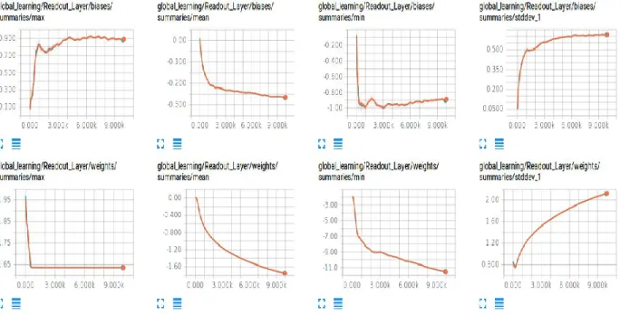
36: MNIST SoftMax Regression Readout Layer Summaries of Global Network………..50
37: MNIST SoftMax Regression Hidden Layer1 Summaries of Global Network………..50
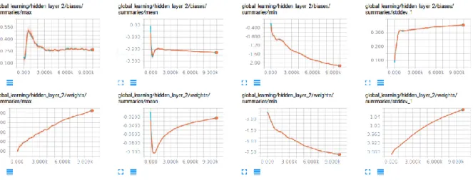
38: MNIST SoftMax Regression Hidden Layer2 Summaries of Global Network………..51
39: MNIST SoftMax Regression Readout Layer Distributions of Global Network………..51
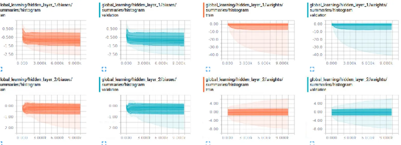
40: MNIST SoftMax Regression Hidden Layer1 and 2 Distributions of Global Network………...52
41: MNIST SoftMax Regression Readout Layer Histograms of Global Network………..52
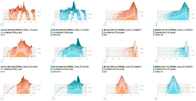
42: MNIST SoftMax Regression Hidden Layer1 and 2 Histograms of Global Network………...53
43: Local Model Confusion – MNIST SoftMax (0, 1, 3, 7, 8)………..54
44: Local Model Confusion – MNIST SoftMax (2, 4, 5, 6, 9)………...55
45: Case 2 Local Model Confusion Table – MNIST SoftMax………..56
x
47: Comparison of Parameters for MNIST Softmax (0, 1, 3, 7, 8) and (2, 4, 5, 6, 9)……….58
48: Case 2 MNIST SoftMax Regression Accuracy Comparison……….58
49: Case 2 MNIST SoftMax Regression Time Comparison………..59
50: Case 2 MNIST SoftMax Regression Accuracy of Global Network………..59
51: Case 2 MNIST SoftMax Regression Cross Entropy of Global Network………..59
52: Case 2 MNIST SoftMax Regression Readout Layer Summaries of Global Network………..60
53: Case 2 MNIST SoftMax Regression Hidden Layer1 Summaries of Global Network………..60
54: Case 2 MNIST SoftMax Regression Hidden Layer2 Summaries of Global Network………..60
55: Case 2 MNIST SoftMax Readout, Hidden1, Hidden2 Layers Distributions of Global Network…….…61
56: Case 2 MNIST SoftMax Readout, Hidden1, Hidden2 Layers histograms of Global Network………….61
57: Comparison of Parameters for MNIST CNN (0, 1, 3, 7, 8) and (2, 4, 5, 6, 9)………..62
58: Local Model Confusion Table – MNIST CNN………63
59: Local Model Confusion – MNIST CNN (0, 1, 3, 7, 8)………64
60: Local Model Confusion – MNIST CNN (2, 4, 5, 6, 9)………64
61: Parameters of Global Network in MNIST CNN DL-DI……….65
62: MNIST CNN Cross Entropy of Global Network………65
63: MNIST CNN Accuracy of Global Network………..66
64: TensorFlow Dataflow Graph for MNIST CNN – Global Network………66
65: MNIST CNN Hidden Layer1 Summaries of Global Network………..67
66: MNIST CNN Hidden Layer2 Summaries of Global Network………..67
67: MNIST CNN Learning Rate of Global Network………67
68: MNIST CNN Readout Layer, Hidden Layer1 and 2 Distributions of Global Network………68
69: MNIST CNN Readout Layer, Hidden Layer1 and 2 Histograms of Global Network………..68
xi
71: MNIST CNN Time Comparison………69
72: Different layers in CIFAR10 Original Solution……….71
73: Architecture of CIFAR10 Original Solution………72
74: Parameters in Different layers in CIFAR10 Original Solution………73
75: Parameters in Local Models of CIFAR10 Using DL-DI……….……74
76: CIFAR10 Local Models Accuracy………..74
77: CIFAR10 Local Model1 Cross Entropy………..75
78: CIFAR10 Local Model1 Raw Cross Entropy………75
79: CIFAR10 Local Model1 Total Loss………75
80: CIFAR10 Local Model1 Raw Total Loss………76
81: CIFAR10 Local Model1 Convolution Summary………..76
82: CIFAR10 Local Model1 Densely Connected Layers Summaries………77
83: CIFAR10 Local Model1 Convolution 1 Distributions………77
84: CIFAR10 Local Model1 Convolution 1 Distributions2………78
85: CIFAR10 Local Model1 Convolution 2 Distributions………78
86: CIFAR10 Local Model1 Convolution 2 Distributions 2………..79
87: CIFAR10 Local Model1 Densely Connected Layer 1 Distributions………79
88: CIFAR10 Local Model1 Densely Connected Layer 1 Distributions 2………80
89: CIFAR10 Local Model1 Densely Connected Layer 2 Distributions………80
90: CIFAR10 Local Model1 Densely Connected Layer 2 Distributions 2………81
91: CIFAR10 Local Model1 Softmax Linear Layer Distributions……….……….81
92: CIFAR10 Local Model1 Softmax Linear Layer Distributions 2……….……….82
93: CIFAR10 Local Model1 Convolution 1 Histograms………..82
xii
95: CIFAR10 Local Model1 Densely Connected 1 Histograms……….………….83
96: CIFAR10 Local Model1 Densely Connected 2 Histograms………..…83
97: CIFAR10 Local Model1 Densely Connected 2……….84
98: CIFAR10 Local Model2 Cross Entropy………..84
99: CIFAR10 Local Model2 Raw Cross Entropy………..85
100: CIFAR10 Local Model2 Total Loss………85
101: CIFAR10 Local Model2 Raw Total Loss……….85
102: CIFAR10 Local Model2 Convolution Summary..……….86
103: CIFAR10 Local Model2 Convolution 2 Summary..……….86
104: CIFAR10 Local Model2 Densely Connected Layers Summaries………86
105: CIFAR10 Local Model2 Convolution 1 Distributions………87
106: CIFAR10 Local Model2 Convolution 2 Distributions………87
107: CIFAR10 Local Model2 Densely Connected Layer 1 Distributions……….87
108: CIFAR10 Local Model2 Densely Connected Layer 2 Distributions……….88
109: CIFAR10 Local Model2 Softmax Linear Layer Distributions………..88
110: CIFAR10 Local Model2 Convolution 1 Histograms………88
111: CIFAR10 Local Model2 Convolution 2 Histograms………89
112: CIFAR10 Local Model2 Densely Connected 1 Histograms………..89
113: CIFAR10 Local Model2 Densely Connected 2 Histograms………..89
114: CIFAR10 Local Model2 Softmax Linear Layer Histograms………..90
115: Parameters of CIFAR10 Global Network……….91
116: TensorFlow Dataflow Graph for CIFAR10 – Global Network……….92
117: TensorFlow Dataflow Graph for CIFAR10 – Global Network Preprocessing………..93
xiii
119: CIFAR10 Global Model Cross Entropy………94
120: CIFAR10 Readout Layer Summaries of Global Network………94
121: CIFAR10 Hidden Layer 1 Summaries of Global Network………..95
122: CIFAR10 Hidden Layer 2 Summaries of Global Network………..95
123: CIFAR10 Hidden Layer 3 Summaries of Global Network………..95
124: CIFAR10 Hidden Layer 4 Summaries of Global Network………..96
125: CIFAR10 Learning Rate of Global Network……….96
126: CIFAR10 Global Model Readout Layer Distributions………..96
127: CIFAR10 Global Model Hidden Layer 1 and 2 Distributions………..97
128: CIFAR10 Global Model Hidden Layer 3 and 4 Distributions………..97
129: CIFAR10 Histograms of Global Network………..98
130: CIFAR10 Global Network Accuracy for Test Data………..99
131: CIFAR10 Global Network Accuracy Table for Test Data………99
132: CIFAR10 Accuracy Comparison………..99
133: CIFAR10 Time Comparison……….100
134: MNIST Softmax Incremental Case Parameter Comparison……….101
135: MNIST Softmax Incremental Case Accuracy Comparison……….101
136: MNIST Softmax Incremental Case Time Comparison………..102
137: MNIST Softmax 3 Local Models Parameter Comparison………..102
138: MNIST Softmax 3 Local Models Accuracy Comparison………..103
139: MNIST Softmax 3 Local Models Time Comparison………103
xiv
ACKNOWLEDGEMENTS
First and foremost, I would like to thank my advisor Dr. Yugyung Lee for all the innovative ideas, insights, advice and challenging deadlines that have helped me achieve this thesis. She has been a constant source of motivation and zeal, not only during my thesis but also during my entire Master program. She was always welcoming for all the help I needed throughout my work, it has always amazed me for the kind of support and inspiring suggestions she has given me for the development of this thesis.
Secondly, I would like to thank the University of Missouri-Kansas City, without which this research would not be possible. The school provided me with good opportunities to support myself and a Lab for my research on a GPU machine. I would also like to thank my lab mates for their generous support.
Finally, I would like to express my heartful gratitude to my family and friends for providing me with constant support and encouragement. This accomplishment would not be possible without them.
1 CHAPTER 1 INTRODUCTION
1.1 Motivation
Machine learning is the science of getting computers to act without being explicitly programmed. It evolved from the study of pattern recognition and computational learning theory in artificial intelligence. Machine learning explores the development of algorithms that can learn from and make predictions on data – such algorithms overcome the traditional software’s following strictly static program instructions especially by making data driven predictions or decisions. Machine Learning algorithm is developed using a training data set and then makes use of this model to answer a question. For example, we can give lot of images of “cat” and “Dog” to build a model and then ask if a new image is cat or dog. Now a days machine learning is used in many use cases, computer vision, speech recognition, natural language processing, language translation, data security, healthcare, marketing, recommendation systems, smart search, self-driving cars, autonomous robots, etc. [15] It is so pervasive today that everybody use it dozens of times a day without knowing it. Many researchers and scholars think it is the best way to make progress towards Artificial Intelligence.
The most powerful form of machine learning being used today, is called “deep learning”, builds
a complex mathematical structure, called neural network, based on large amounts of data. Neural networks are designed to work analogous to how a human brain works. Neural networks were first described in 1930’s but only in the last four to five years, enough computational power has been achieved. But it takes a massive amount of computing performance to train the sophisticated deep neural networks that power these new applications. It’s a huge challenge. Training can take days to weeks to months on even the fastest supercomputers. There are lot of advancements in GPU computations recently. With GPU acceleration [10], neural networks training is 10-20 times faster than with CPUs. Because of this training time is decreased from days or even weeks to some hours. This lets
2
developers and data scientists build larger, more complex neural networks, which leads to incredibly intelligent next-generation applications. NVIDIA GPUs [10] and the Deep Learning SDK are driving advances in machine learning. The number of organizations developing and using GPU-accelerated frameworks to train deep neural networks is growing. As the number of applications is growing, the number of models used are also growing in more heterogenous manner. That is models with different applications need to combined and sometimes only part of some models might be needed. Data is growing enormously each day, currently ImageNet [21] a hierarchical image database contains 14,197,122 images and growing each day. Because of this there is a need for more scalable, distributed learning, incremental, multi task able machine learning approach. This research presents one such approach, which is scalable with distributed learning and incremental properties.
1.2 Problem Statement
Most of the machine learning algorithms today, especially in deep learning try to solve a supervised classification problem whether it is computer vision or natural language processing. A supervised classification model tries to classify an input to one of the pre-labeled classes or categories.
For example, classifying an image whether it is a “cat” or “dog”. Some of the research questions for distributed deep learning are: can we distribute learning tasks to multiple CPU/GPU machines while minimizing loss? Distributing learning and recognition through data parallelism, model parallelism and task parallelism. Data parallelism is to use same model in entire cluster but use different data in each machine. Model parallelism is use to same data across all machines in cluster but split the model across cluster. Task parallelism is to distribute different tasks to different machines in cluster.
The model training can be distributed with current architectures, i.e. distributed computing is available with the existing libraries like TensorFlow, Caffe, Apache Spark, etc. But it is not possible to do distributed learning or inference by following traditional model approaches. Using a complex deep
3
network model for inference would need operations in range of millions. A model inference which can be distributed is required for better performance.
As the data grows, model needs to learn about this new data. For example, in recommendation and user behavior systems, a model needs to update based on user preferences which change time-to-time. In traditional approaches, the complete end-to-end model needs to be retrained for new data. The existing model needs to be replaced completely. If we would like to add a new class or category to the existing model, then the model needs to be completely redesigned and trained from scratch. Existing approaches does not fully support incremental deep learning for building models that can evolve efficiently with new designs, data and requirements from users.
Complex models are being developed to increase the model’s predictive performance. These
complex solutions often involve using multiple models, for example, audio and visual input for image classification. Such implementations need more distributed approaches. With advancements in machine learning algorithms, user expectation also grows and this leads to creating models which can perform multiple tasks for which we need to combine many of the existing machine learning algorithms.
1.3 Proposed Solution
This thesis presents a machine learning framework that is scalable, distributed and incremental in nature. The presented approach focuses mainly on an image classification problem, but can be applied to most other supervised machine learning problems.
At a higher level of abstraction, the machine learning problem is divided into two parts hierarchically. In the first part of the learning, all the classes or categories are divided into smaller sets of heterogeneous groups. This group size can be in different ranges, but should be a minimum two for a classification problem. These smaller sets of heterogenous classes is again a supervised classification problem, but with the smaller number of classes. These smaller classification problems are solved using traditional machine learning algorithms. For example, image classification sub-problem can be solved
4
using Convolutional Neural Networks [11, 23, 24, 27]. For the second part of the problem, predictions made by the smaller models is used as input to solve the overall prediction task. In the second part of problem, additional machine learning algorithms different from the original solution are used to solve the complete classification problem. Because of the less number of input dimensions for the second part, and based on the number of groups, size of the groups and heterogeneity of these groups, the problem in the second part can be complex enough but it would not increase with different requirements.
The approach makes use of SoftMax regression [38], Convolutional Neural Networks, Random Forest, etc. machine learning techniques. TensorFlow [36], open source software library for numerical computation and machine intelligence is used. The proposed approach can be extended to solve for most other supervised problems like natural language processing, language translation, speech recognition. The evaluation on several case studies is presented to verify that the DL-DI framework supports distributed incremental deep learning while achieving a reasonably high rate of prediction accuracy.
5 CHAPTER 2
BACKGROUND AND RELATED WORK
In this chapter, we will learn the terms that have been used throughout the paper and introduce the background technologies. We will also discuss the related works to the presented solution and problem statement.
2.1 Terminology and Technology
2.1.1 Machine Learning
Machine learning is the science of getting computers to act without being explicitly programmed. This subfield evolved from the study of pattern recognition and computational learning theory in artificial intelligence. Machine Learning explores the development of algorithms that can learn from and make predictions on data. Traditional algorithm follow static program instructions. Machine learning overcomes this by making data driven predictions and decisions. Machine Learning algorithm is developed using a training data set and then make of this model to answer a question.
“A computer program is said to learn from experience E with respect to some class of tasks T and performance measure P, if its performance at tasks in T, as measured by P, improves with experience E. Machine learning tasks are typically classified into three broad categories, depending on the nature of the learning "signal" or "feedback" available to a learning system.” [17]
Supervised learning is a type of machine learning algorithm that uses a known dataset (called the training dataset) to make predictions. The training dataset includes input data and response values. From it, the supervised learning algorithm trains itself to build a model that can make predictions or responses for new data with similar attributes. A test dataset which is not used during training of model is used to better validate the model. Using larger training datasets often results in models with higher accuracy or predictive capability that can generalize well for new data.
6
Classification: In this supervised problem algorithm needs to produce categorical response values, where the data can be separated into specific “classes” or groups.
Regression: In regression, algorithm tries to predict for continuous-response values
Unsupervised Learning: It is a type of machine learning algorithm used to get inferences from datasets consisting of input data without labeled responses i.e., without response values. The most common unsupervised learning method is cluster analysis, which is used for exploratory data analysis to find hidden patterns or grouping in data. The clusters are modeled using a measure of similarity which is defined upon metrics such as Euclidean or probabilistic distance.
2.1.2 Neural Networks
The study of artificial neural networks (ANNs) has been inspired in part by the observation that biological learning systems (e.g., human brain) are built of very complex networks of interconnected neurons (Figure1 and Figure2). In an analogy, artificial neural networks are built out of a densely interconnected set of simple artificial neuron units, where each unit takes several inputs (usually the outputs of other units) and produces a single or several real-valued outputs (which may become the input to many other neurons). The human brain, for example, is estimated to contain a densely interconnected network of approximately 1011 neurons, where each neuron is connected, on average, to 104 others. While ANNs are loosely motivated by biological neural systems, there are many complexities to biological neural systems that are not modeled by ANNs, and many features of the ANNs we discuss here are known to be inconsistent with biological systems. But still, the overall network architecture is sometimes modelled again similar to biological systems.
7
Figure 1: Cartoon Drawing of a Biological Neuron [3]
Figure 2: Mathematical Model of Biological Neuron [3]
ANN system is based on a simple unit called a perceptron (Figure 3). A perceptron is an artificial neuron. A perceptron takes a vector of real-valued inputs, calculates a linear combination of these inputs, then outputs a 1 if the result is greater than some threshold and -1 otherwise.
Output= {0 𝑖𝑓 ∑ 𝑤𝑗 𝑗𝑥𝑗≤ 𝑡ℎ𝑟𝑒𝑠ℎ𝑜𝑙𝑑 1 𝑖𝑓 ∑ 𝑤𝑗 𝑗𝑥𝑗> 𝑡ℎ𝑟𝑒𝑠ℎ𝑜𝑙𝑑
8
Figure 3: Mathematical Model of Artificial Neuron [3]
This function is called “activation function”. Different types of activation functions are: Sigmoid: The Sigmoid non-linearity has the following mathematical form
𝑦 =
σ(x) =
1
1 + 𝑒𝑥𝑝
−𝑥It takes a real value and outputs between 0 and 1. However, the neuron's activation saturates at either tail of 0 or 1, the gradient at these regions is almost zero.
Hyperbolic Tangent: The TanH non-linearity has the following mathematical form
𝑦 = 2𝜎(2𝑥) − 1
It squashes a real-valued number between -1 and 1.
Rectified Linear Unit: The ReLU has the following mathematical form
𝑦 = max (0, 𝑥)
The ReLU has become very popular in the last few years, because it was found to greatly accelerate the convergence compared to the sigmoid, tanh, etc. functions because of its linear and non-saturating form above zero. In fact, it does not suffer from the vanishing or exploding gradient. Another advantage is that it involves cheap operations compared to the expensive exponentials. However, the
9
ReLU removes all the negative information and thus appears not suited for all datasets and architectures.
Figure 4: Different Activation Functions [18]
Logistic Regression: It calculates the mathematical relationship between the categorical (class labels or response value) dependent variable and one or more independent variables (input values or attributes) by estimating probabilities using a logistic function, which is the cumulative logistic distribution. It classifies to only two classes i.e. binary classification. A sigmoid neuron can be used to make a logistic regression model since it exactly models a logistic regression problem.
SoftMax Regression: It (or multinomial logistic regression) is a generalization of logistic regression where we want to apply for multiple classes. In logistic regression, we assumed that the class labels were binary i.e. either “Yes” or “No”. Softmax regression allows us to handle K number of classes. Instead of one sigmoid neuron we would have to use K number of Sigmoid neurons.
10
Multilayer Perceptron: A neural network is put together by hooking together many of our
simple “neurons,” sending the output of a neuron as input to other neurons. A multilayer perceptron (MLP) is a feed-forward artificial neural network model that takes a set of input data and gives a set of outputs as either categorical or continuous values. An MLP consists of multiple layers of neurons in a directed graph, with each layer fully connected to the next one. Except for the input nodes, each node is a neuron (or processing element) with a nonlinear activation function explained above. It utilizes a supervised learning technique or algorithm called backpropagation for training the network. It is called feed forward because as we proceed in the network, output of one layer is given as input to the next layer and there are no cycles.
Figure 5: Example Feed Forward Multi-Layer Perceptron [18]
In Figure 5, leftmost layer of the network is called the input layer, and the rightmost layer the output layer (which, in this example, has only two nodes or neurons). All the middle layers of nodes are called the hidden layers, because its values are not observed in the training dataset. Example neural network (Figure 5) has 3 input units (not counting the bias unit), 3 hidden units in one layer and 2 hidden units in another layer, and 2 output units.
11
Using forward step progress, feed forward network can be built as follows:
𝑎1 (2)= 𝑓 (𝑊11(1)𝑥1+ 𝑊12(1)𝑥2+ 𝑊13(1)𝑥3+ 𝑏1(1)) 𝑎2 (2)= 𝑓(𝑊21(1)𝑥1+ 𝑊22(1)𝑥2+ 𝑊23(1)𝑥3+ 𝑏2(1)) 𝑎3 (2)= 𝑓(𝑊31(1)𝑥1+ 𝑊32(1)𝑥2+ 𝑊33(1)𝑥3+ 𝑏3(1)) ℎ𝑊,𝑏 (𝑥) = 𝑎1 (3) = 𝑓(𝑊11(2)𝑎1(2)+ 𝑊12(2)𝑎2(2)+ 𝑊13(2)𝑎3(2)+ 𝑏1(2)
Feed forward outputs:
𝑧(2)= 𝑊(1)𝑥 + 𝑏(1) 𝑎(2) = 𝑓(𝑧(2)) 𝑧(3)= 𝑊(2)𝑎(2)+ 𝑏(2) ℎ𝑊,𝑏 (𝑥) = 𝑎(3)𝑓(𝑧(3))
2.1.3 Convolutional Neural networks
Spatial Convolution: Regular Neural Networks (Multilayer Perceptron), only made of linear and activation layers, do not scale well to images which has spatial features and large number of input dimensions. For instance, images of size 3 × 224 × 224 (3 color channels, 224 wide, 224 high) would necessitate a first linear layer having 3 * 224 * 224 + 1 = 150; 129 parameters for a single neuron (e.g. output). Spatial convolution layers take advantage of the fact that their input (e.g. images or feature maps) exhibits many spatial relationships. In fact, neighboring pixels should not be affected by their location within image. Thus, a convolutional layer learns a set of Nk filters F = f1, …, fNk, which are convolved spatially with input image x, to produce a set of Nk 2D features maps z:
Zk = fk * x
where * is the convolution operator. When the filter correlates well with a region of the input image, the response in the corresponding feature map location is strong. Unlike conventional linear layer, weights are shared over the entire image reducing the number of parameters per response and
12
equivariance is learned (i.e. an object shifted in the input image will simply shift the corresponding responses in a similar way). Also, a fully connected layer be a convolutional layer with filter of sizes 1 x 1 x input size. It is important to highlight that a spatial convolution is not defined by the spatial size of the input feature maps (e.g. wide and high), neither by the size of the output feature maps, but by the number of filters (e.g. number of output channels), the properties of its Filters (e.g. number of input channels, wide, high) and the properties of the convolution (e.g. padding, stride).
Spatial Pooling: In Convolutional Neural Networks, a pooling layer is typically present to provide invariance to slightly different input images and to reduce the dimension of the feature maps (e.g. wide, high):
pR = Pi∈R (zi)
where P is a pooling function over the region of pixels R. Max pooling is preferred as it avoids cancellation of negative elements and prevents blurring of the activations and gradients throughout the network since the gradient is placed in a single location during backpropagation.
The spatial pooling layer is defined by its aggregation function, the high and width dimensions of the area where it is applied, and the properties of the convolution (e.g. padding, stride).
Figure 6: Illustration of a Spatial Pooling Operation in 2 x 2 Regions by a Stride of 2 in the High Direction, and 2 in the Width Direction, Without Padding. [42]
13
Batch Normalization: This layer quickly became very popular mostly because it helps to converge faster. It adds a normalization step (shifting inputs to 0 mean and standard unit variance) to make the inputs of each trainable layers comparable across features. By doing this it ensures a high learning rate while keeping the network learning. Also it allows activations functions such as TanH and Sigmoid to not get stuck in the saturation mode (e.g. gradient equal to 0).
Many convolution architectures have been developed from 1990’s, we will present few of
them.
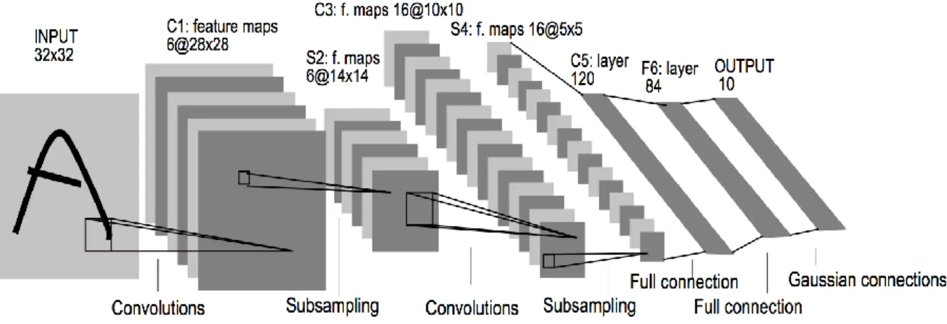
LeNet: This kind of architecture is one of the first to successfully implement CNNs. It was developed by Yann LeCun in the 1990's and was used to read zip codes and hand written digits. This architecture, about the modern ones, differs on many points. Thus, we will limit ourselves on the most known, LeNet-5 [11], and we will not delve into the details. In overall this network gave path to much of the recent convolutional architectures, and a true inspiration for many people in the field. LeNet-5 network features can be summarized as:
sequence of 3 layers: convolution, pooling, non-linearity,
inputs are normalized using mean and standard deviation to accelerate training,
sparse connection matrix between layers even after convolutions to avoid large computational cost
hyperbolic tangent or sigmoid as non-linearity function,
trainable average pooling as pooling function,
fully connected layers as final classifier,
14
Figure 7: Architecture of LeNet-5, an Old Convolutional Neural Network for Digits’ Recognition. [13]
AlexNet [11]: It is another one of the first work that popularized convolutional networks in computer vision and image analysis. AlexNet was submitted to the ImageNet ILSVRC challenge of 2012 and significantly outperformed the other hand crafted models (accuracy top5 of 84% compared to the second runner-up with 74%). This network, compared to LeNet, was deeper (60 million of parameters) and bigger (5 convolutional layers, 3 max pooling layers and 3 densely-connected layers). At this implementation, the authors provided a multi-GPUs implementation in CUDA to bypass the memory needs. It popularized:
the ReLU as non-linearity function of choice,
the method of stacking convolutional layers plus non-linearity on top of each other without being immediately followed by a pooling layer,
15
Figure 8: An Illustration of the Architecture of AlexNet. One GPU Runs Layer-Parts at the Top of Figure While the Others Run the Layer-Parts at the Bottom. [11]
VeryDeep or VggNet [23]: It was the runner-up architecture of ILSVRC2014 with almost 140 million of parameters. Its main contributions were to show that depth is a critical component for good performance, to use much smaller 3 x 3 filters (helps in identifying better features) in each
convolutional layer, and to combine them as a sequence of convolutions. The great advantage of VggNet was the insight that multiple 3 x 3 convolution in sequence can increase the effect of larger receptive fields, for example 7 x 7 and 5 x 5. These ideas of using a sequence of smaller filter layers is used in more recent CNN architectures such as Inception [7].
16
GoogLeNet or Inception [7]: It was the winner architecture of ILSVRC2014. Its main difference was the usage of an Inception Module that dramatically reduced the number of parameters (40 millions). Also, it eliminated many parameters by using average pooling instead of densely connected layers after the output of the convolutional layers. Further versions of the GoogLeNet has been released. The most recent architecture available is InceptionV3. Notably, it uses batch normalization.
Figure 10: 1 x 1 Convolutions are Used to Decrease the Input Size Before 3 x 3 Convolutions to Provide more Combinational Power Such as in GoogLeNet [7].
2.1.4 Model Training
Initialization: Initialize weights with a small amount of noise to break symmetry across trained parameters, and to prevent vanishing gradients. If ReLU neurons are used, it is always a good practice to initialize biases with a slightly positive initial bias to avoid "dead neurons".
Loss Function: To quantify the capacity of the network to approximate the ground truth labels for all training inputs, we define a loss function which takes as inputs the weights, biases, and
examples from the training set. For instance, the loss could be the number of images correctly classified. However, the most efficient way to find the weights and biases, regarding the number of parameters, is to use an algorithm like the Stochastic Gradient Descent (SGD). To do so, if our chosen loss function is not smooth, we must choose a surrogate loss (e.g. derivable function) such as Mean Square Error or Cross Entropy.
17
Backpropagation: For each example, we compute the prediction and its associated loss. We sum up all the loss to compute the final error. Then we use the backpropagation algorithm to propagate the error to compute the partial derivatives
𝛿𝐸 𝛿𝑤 𝑎𝑛𝑑
𝛿𝐸 𝛿𝑏
of the cost function E for all weights w and bias b. In this work, our goal is not to explain in details how works the backpropagation algorithm. More information is available in Chapter 2 of Michael Nielsen's book [27].
Optimization: Once all the derivatives are computed, we update our parameters using a chosen optimization technique such as SGD. We then iterate the predication (e.g. forward pass), the backpropagation of errors (e.g. backward pass) and the optimization until convergence hopping to find a local minimum low enough to ensure good predictions. Even if the chosen surrogate loss function of a neural network is non-convex, SGD works well in practice. There are many other optimization techniques available: Gradient Descent, Nesterov accelerated gradient, Momentum, Adagrad, Adadelta, RMSProp, Adam (Adaptive Moment Estimation). In this research, we used several of these based-on requirements to achieve faster and good convergence.
Grid Search: It is common to explore manually the space of hyperparameters such as learning rate, weight decay, learning rate decay, amount of dropout, not to mention the architecture hyperparameters, to obtain the best performance in terms of both accuracy and training time. Going deeper with convolutions [24] made an evaluation on the influence of architecture choices and optimization hyperparameters on ImageNet. Most of the current research implementations used grid search to find appropriate hyperparameters.
Regularization: Deep and large enough neural networks can memorize any data. During training, their accuracy on the trainset typically converges towards perfection while it degrades on the test set. This phenomenon is called overfitting. To reduce this a range of regularization techniques can
18
be used. L2 Regularization, data augmentation, dropout, drop connect, early stopping. For most of the current implementations we used Dropout.
Dropout: The idea is to randomly set a certain percentage of the activations in each layer to 0. During the training, neurons must learn better representations without co-adapting to each other being active. At each training step in a mini-batch, the dropout procedure creates a different network (by randomly removing some units), which is trained using backpropagation as usual. The effect of this is that neurons are prevented from co-adapting too much which makes overfitting less likely. At test case the whole network is used (all units) but with scaled down weights. Mathematically this approximates ensemble averaging (using the geometric mean as average). It can also be said as a form of ensemble learning.
2.2 TensorFlow
TensorFlow is an open source software library for numerical computation using data flow graphs. Nodes in the graph represent the mathematical operations to be computed. Graph edges represent the data communicated between nodes in graph in the form of multidimensional data arrays called tensors. The flexible architecture allows us to deploy computation to multiple machines one or more CPUs or GPUs in a desktop, server, or mobile device with a single API provided by Google. TensorFlow was developed by Google brain Team for conducting Google’s Machine Intelligence
research but it is general enough to be applicable for several other domains if applied right.
TensorFlow is designed for large-scale distributed training and inference, it can be used for experimenting with machine learning models. The TensorFlow runtime is a cross-platform library which can be used across desktop, mobile, etc. Figure 11, illustrates its architecture supporting different programming languages and devices. TensorFlow has a layered architecture. A C API separates user level code written in different languages from the core runtime kernels. Kernel implementations are on
19
top of Networking and Device layer. Master and Dataflow executor are above kernel implementations. TensorFlow gets its parameter server architecture from DistBeleif [7].
Figure 11: TensorFlow Architecture [36]
Data flow graph is the main abstraction that is used to describe the mathematical computation with a directed graph of nodes and edges.
Nodes in the graph represent mathematical operations
Edges in the graph describe the i/o relationships between several operations
Data edges in the graph carry dynamically-sized multidimensional data arrays called tensors The flow of tensors is where TensorFlow gets its name. Nodes are assigned to different computational devices and can be executed asynchronously, in parallel once all the tensors on their incoming edges become available. This design helps us to make model more distributed and parallelism is only distributed computing with a dependency to incoming edges. This dependency needs to be reduced.
20
Figure 12: Example TensorFlow dataflow graph [36]
Computation Graph: TensorFlow programs are usually written in two stages, a construction phase, that assembles a graph using multiple operations as nodes and dataflow as edges, and an execution phase that uses a session to execute the operations in the graph using core libraries. Usually, a graph is first constructed to train a graph and using this the network is trained by running these ops in a loop in the execution phase. TensorFlow can be used from C, C++, and Python programs. It is presently much easier to use the Python library than C library to assemble graphs in construction phase, as it provides a large set of helper functions which are not yet available in the C and C++ libraries. TensorFlow is also available in Java but it is still in experimental stage. For now, we will use python to construct the graphs. TensorFlow Python library has a default graph to which ops constructors add nodes. The default graph is sufficient for many applications. TensorFlow allows interactive run, that is it allows to move execution between python or client and back end. But to make use of GPU computations effectively it is better to not move the execution between python and back end at least for the training phase.
Tensors: TensorFlow programs use a tensor data structure to represent all data -- only tensors are passed between operations in the computation graph. You can think of a TensorFlow tensor as an n-dimensional array or list. A tensor has a static type, a rank, and a shape. Python lists, arrays, numpy lists and arrays can be feed to graph or converted to tensor objects using helper functions in python.
21
Variables: Variables maintain state across executions of the graph. Required to update model parameters.
TensorBoard: The computations you'll use TensorFlow for - like training a massive deep neural network - can be complex and confusing. TensorBoard is a visualization tool which is part of TensorFlow libraries. It can be used to understand, debug, and optimize programs. Using TensorBoard we can visualize the complete graph, various metrics like mean, min, max, standard deviation of variables,
activations of neurons intermediate data, images, distributions, embedding’s, etc. The data displayed with TensorBoard module are generated during the execution of TensorFlow and stored in log files whose data are obtained from the summary operations.
GPU Usage: Because of the more number of cores and higher parallelism, using GPU accelerates the Deep Learning Routines. Deep Learning Networks, Convolutional Networks most used operations are Matrix, vector multiplications, convolutions, and other small set. GPU can be used to accelerate these operations to reduce training time. NVIDIA Deep Learning SDK provides powerful tools and libraries for designing and deploying GPU accelerated deep learning applications. It contains many libraries and tools like cuDNN, GIE, CUDA toolkit, etc. cuDNN provides highly tuned implementations for standard routines such as forward and backward convolution, pooling, normalization, and activation layers. GPU Inference Engine (GIE) optimizes your trained neural networks for runtime performance. Deep Learning GPU Training System (DIGITS) helps in designing the best deep neural network (DNN) for image classification and object detection tasks using real-time network behavior visualization.
2.3 Related Work
This research focuses on building multiple heterogenous models and combining their predictions in another model. The easiest comparison one would make with this approach is ensemble learning. There are three most used ensembles learning methods are Bagging, Boosting and Voting [41]. Bagging is to Build multiple machine learning models (generally of the same type) from different
22
subsamples of the training dataset. Boosting is also to build multiple models (again generally of the same type) each of which learns to fix the prediction errors or loss of a prior model in the chain. Voting is to build multiple models (typically of differing types) and simple statistics (like calculating the mean) are used to combine predictions. All these approaches build many models most of the time for all the classes with different subset of data. But our approach is to build smaller models with heterogenous classes and then combine their prediction.
Figure 13: Comparison of DL-DI and Other Related Works
MLDD [22] discusses a Multi-Level discriminative dictionary learning with application to large scale image classification. They incorporated the discrimination of classification task into dictionary learning. Sparse local features (like SIFT features) are used as input to build dictionary. The input image is represented using the dictionary that is built. It takes advantage of category hierarchy for discriminative dictionary learning. The classes are arranged as a tree hierarchically. In the tree, root node contains all classes, and leaf nodes corresponds to single classes. Internal nodes correspond to a hyper-category, a set of associated classes. This hierarchy is built using correlation or visual similarity
23
for image classification. The overall tree loss is reduced using gradient descent optimizations. There are a lot of differences between this and our presented approach. The proposed approach uses only two levels how large the number of categories are. Our approach can be said as bottom-up hierarchy to make the final predictions this is where our approach is similar to this approach, we are using a hierarchy to improve model properties in terms of scalability, distributed learning and inference and incremental learning. Start with smaller heterogenous models and then go to next part of model which makes final predictions based on predictions from a smaller model. We are not using any dictionaries and sparse features like SIFT. We are using pixel data as input features. In our approach, local models are trained with individual losses and the second part of model is trained with another loss function.
David H. Wolpert introduced stacked generalization [26], a scheme for minimizing the generalization error rate of one or more generalizers. It also uses multiple models built on same data. Each model may make a partial guess or higher level predictions and there will be other models to give final predictions. Unlike bagging and boosting, stacking may be (and normally is) used to combine models of different types. Using disjoint sets of training data, base learners are built and a higher-level learner is built to make the final predictions. By far this approach may look very similar to what we are doing but in stacked generalization each base learner is modelled on all the classes and in our approach, we build several smaller models on heterogenous groups. This makes our approach significantly different in terms of the end-to-end system.
Figure 13 provides a comparison between Deep Learning Distributed, Incremental (DL-DI) framework and recent work in distributed deep learning from companies like Google, Microsoft, NVIDIA. DistBeleif, COTS HPC, Project Adam, MLDD approaches achieve distributed computing for deep learning by using asynchronous parameter update, shared system state, neural network decomposition. They have a lot of dependency and latency due to network usage. Some of these use advanced networking techniques to improve distributed computing but none of these supports
24
incremental deep learning inherently to the extent that is required. SINGA [19] does neural network partition along the edges of the graph increasing the dependency. All these achieve distributing computing by using data parallelism or model parallelism. Data parallelism is to use same model in entire cluster but use different data in each machine. Model parallelism is use to same data across all machines in cluster but split the model across cluster. Rudra [8] is a parameter server based deep learning frame work and they did a systemic study to on trade-off between model accuracy and run-time or parallelism. They also checked interdependencies between hyper parameters in a distributed setting. They concluded that there is a limit on parallelism that can be done in such frameworks for image classification. With the DL-DI framework there is very less dependency between different parts of the network and neural network is decomposed such that in a eco system, using different models there would be advantage. The distributed, incremental learning properties are inherent in the DL-DI framework.
25 CHAPTER 3
The DL-DI Framework
3.1 Overview
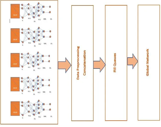
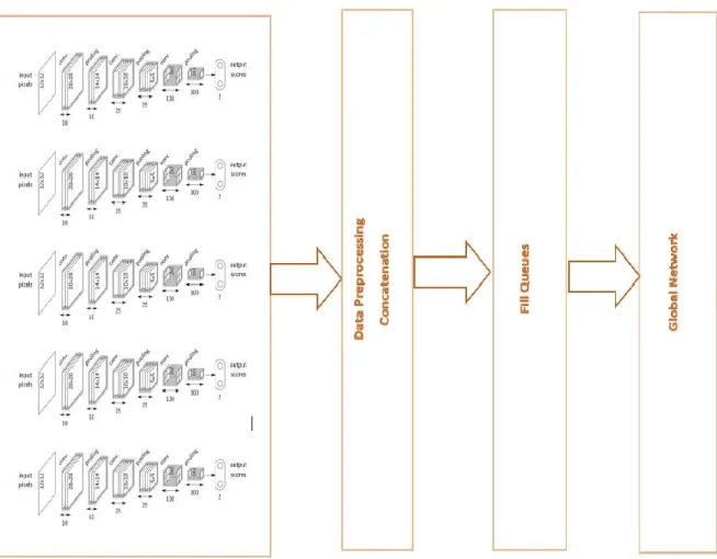
The proposed solution works for any type of supervised learning problem, we will the design of framework for Image Classification. The overall architecture is presented in Figure 14. The supervised learning problem is divided into two stages, Local Learning and Global Learning. As a classification problem, we will have a set of classes, these are divided into some smaller heterogenous groups. That is classification problem is divided into sub problems. Local Learning is to solve these sub problems using traditional approaches, i.e. a feed-forward network or a Convolutional Neural Network [11, 23, 24, 27]. As we would be solving small number of categories in each sub problem the number of parameters that are need will be less and name these as local models. Once the local learning is completed, we will make use of the predictions of local models as input for the global learning. Global learning problem is to give the overall prediction based on the predictions made by local models. For this problem, another neural network is built, the size and complexity of this network will be based on the overall problem complexity, in this case the number of classes in the overall classification problem. For the problem of Image Classification, a fully connected feed-forward network will be required. The number of hidden layers varies based on number of classes. Additional tuning on this global neural network model need to be done for better performance.
3.2 Local Learning
Overall classification problem is divided into smaller problems and these smaller problems are solved using a neural network similar to original solution with small problem size. The size of the smaller problem and the number of smaller groups are decided based on our future needs like how small the
26
sub-problem needs to be and how often new classes are added to the model, how often new data is added,
Figure 14: Proposed DL-DI Framework for Image Classification
how sparse the new data to be added is, etc. For example, if the overall classification problem has 10 classes, then we can divide it in to 5 sub-problems of two classes or 2 sub-problems of 5 classes in each or several other combinations. We will choose these based-on future requirements to support incremental, distributed nature with minimal computational expenses. Then select the sub-problem size and group size based on following:
How frequent new classes are added.
How frequent new data is added to existing classes.
How sparse the new data will be. Out of all the available classes, for how many classes does new data is updated.
27
If none of the above scenarios are not needed, then a more intriguing method of identifying patterns in features can be used to find the clusters. We can distribute these classes while optimizing overall learning outcome. Multi-class Discrimination Distribution Model [4] is used to find the appropriate clusters. Distribute the classes based on the evidence of classification confusion from confusion matrix. Then the degree of heterogeneity between classes is found by calculating measurements such as Euclidean distance, etc. for precision, recall, F-measure matrices. The complete process is:
Classes are distributed based on the evidence of classification confusion from the Confusion matrix. Algorithm of Hierarchical Distribution:
Step 1: Classification with the original dataset
Step 2: The degree of heterogeneity computed by several measurements such as Euclidean distance (ED) or normalized ED for Confusion matrices, Precision, Recall, F-measure matrices
Step 3: K-means clustering with the matrices (K= √𝑛, 𝑛 is the 𝑛𝑢𝑚𝑏𝑒𝑟𝑜𝑓𝑐𝑙𝑎𝑠𝑠𝑒𝑠) Step 4: Classification on the k matrices (distributed classification)
Repeat until the accuracy < threshold or √𝑛 <4
The visual representation of the MCDD model is shown in Figure 15.
28
For solving the sub-problems, we will use lesser number of parameters, making each local model less complex than the existing model for overall problem. A less complex model should be enough to solve the sub-problem and the accuracy and performance of local problem would be better because of the smaller problem size.
Consider the classification of MNIST computer vision dataset as an example. It consists of hand written images of numbers 0 to 9. The MNIST dataset consists of three parts: 55,000 images of training data, 10,000 images of test data, and 5,000 images of validation data. Every MNIST data point has two parts: an image of a handwritten digit and a corresponding label. All the data contain images and their corresponding labels. Each image is 28 pixels by 28 pixels. We can interpret this as a big array of numbers as shown in Figure 17.
Figure 16: Examples from MNIST Dataset [36]
29
This two-dimensional array can be flattened in to a single vector of 28x28 = 784 numbers. So MNIST images can be represented as points in a 784-dimensional vector space. The training dataset is a tensor with a shape of [55000, 784]. The first dimension is an index to the number of images in the dataset and the second dimension contains actual image pixels.
The labels can be represented as “one-hot” encoders. In the one-hot encoding the number of dimensions in label data will be equal to number of classes. Each dimension corresponds to that class and for a data point only one of all the dimensions will be one and others will be zero. The label data is a tensor of shape [55000, 10] for training dataset.
Consider solving this problem using simple Softmax Regression As shown in Figure 18 (shows a Softmax regression for 3 inputs and 3 outputs) and Figure 19 (784 input neurons and 10 output neurons). When we try to solve this, our weight variable will be of shape [784,10] (since 10 output neurons for 10 classes) and bias variable of shape [10]. Then we define a loss function, say cross entropy and update our weights and biases using an optimizer (like gradient descent) to reduce this loss.
30
Figure 19: Architecture of MNIST SoftMax Regression
If we want to solve the same MNIST classification problem using our approach, we would want to design sub-problem size and number of groups (i.e. group size). For example, say 2 classes in each sub-problem, then there will 5 such groups. These heterogenous groups can be as [(0,1), (2,3), (4,5), (6,7), (8,9)]. There are several other combinations, these heterogenous groups can be selected based on the confusion matrix from original model. Say we designed the heterogenous groups as [(0,1), (2,3), (4,5), (6,7), (8,9)], then for each sub-problem we would need a weight variable of shape [784,2] and bias variable of shape [2] with the Softmax regression. Since there are only 2 classes in each sub-problem higher accuracy can be achieved with less number of iterations than that is required in original model. The local learning is to solve sub-problem with same approach as original solution of the problem with optimal number of parameters and performance.
This MNIST classification problem can also be solved using Convolutional neural network to achieve higher accuracy because using convolutional neural network we can make use of the spatial features in images. Let us look at the sample design of original CNN model for MNIST classification problem.
31
• Each convolutional layer contains one convolution and max pooling.
• Convolutional layers, one densely connected layer, one dropout layer, read out layer
• First convolution layer contains 32 features for each 5x5 patch. The weight variable is of shape [5, 5, 1, 32] and bias variable of shape [32] with [1,1,1,1] strides and for pooling ksize = [1, 2, 2, 1], strides = [1, 2, 2, 1].
• Second convolution layer contains 64 features for each 5x5 patch. The weight variable is of shape [5, 5, 32, 64] and bias variable of shape [64] with [1,1,1,1] strides and for pooling ksize = [1, 2, 2, 1], strides = [1, 2, 2, 1].
• Densely connected layer will have weight variable of shape [7*7*64,1024] and bias variable of shape [1024].
• Readout layer will have weights of shape [1024, 10] and biases of shape [10]
Then we define a loss like cross entropy, use an optimization algorithm to update parameters reducing loss and increasing accuracy. This original solution is presented in Figure 20.
32
If we want to solve the same MNIST classification problem using our approach, we would want to design sub-problem size and number of groups (i.e. group size). Say we designed the heterogenous groups as [(0,1), (2,3), (4,5), (6,7), (8,9)], then each sub-problem can be solved as follows:
Each convolutional layer contains one convolution and max pooling.
2 Convolutional layers, one densely connected layer, one dropout layer, read out layer
First convolution layer contains 6 features for each 5x5 patch. The weight variable is of shape [5, 5, 1, 6] and bias variable of shape [6] with [1,1,1,1] strides and for pooling ksize = [1, 2, 2, 1], strides = [1, 2, 2, 1].
Second convolution layer contains 12 features for each 5x5 patch. The weight variable is of shape [5, 5, 6, 12] and bias variable of shape [12] with [1,1,1,1] strides and for pooling ksize = [1, 2, 2, 1], strides = [1, 2, 2, 1].
Densely connected layer will have weight variable of shape [7 * 7 * 12, 100] and bias variable of shape [100].
Readout layer will have weights of shape [1000, 10] and biases of shape [10]
The design of local models is made such that the total parameters are in the same range as original model i.e., there is no increase in the number of parameters for local models and the number of iterations required to solve sub-problems will be lesser than the original solution and the accuracy of local models would be high. This approach can be extended to any type of supervised learning problem. This approach can be extended to join different local model problems i.e., say image classification and text classification, or image and speech classifier to solve a multi-task model problem. This is scalable because the number parameters, time to computation is similar. Because of this we can include distributed and incremental learning properties in our approach.
33
3.3 Global Learning
Global learning tries to solve the overall classification or prediction problem based on inputs from local model. It consists data preprocessing, selecting different hyper parameters like number of neurons, layers, regularization.
Data Preprocessing: Input to global model comes from local models. We would have to combine the results from all the local models. We should do other pre-processing on input data like batch preparation, queue preparation, etc. such that it is ready to be provided to global model. In our approach, we send local model predictions as input to global model. For all the available training data, compute local predictions first. For this we would have to load all local models and compute local model predictions. Then prepare queue of this data for global model such that it won’t wait for input data. For
the global learning, we could send in the final layer activations as input instead of simple Softmax predictions for higher performance of global model. If we want to join different kinds of local models, then the data preprocessing would include proper vector transformations required based-on the type models being joined. Labels for global model would be same as for overall problem. Most of the
scenario’s the preprocessing would include following:
• Freeze local model graphs and load them to default graph.
• Compute local model predictions or required local model activations.
• Combine the local model responses into single input vectors
• Create functions to generate batch data and fill queues with data
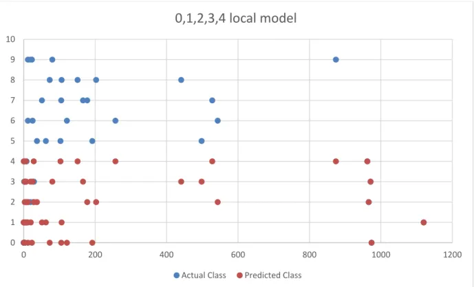
Local Model Confusion: Local models are trained to classify for sub-problems, but for global model we need compute predictions from local models for all classes data and local model may not able to always classify one class data into one of the trained classes. For example, a local model trained to classify between (0,1) may be able to classify all 3’s to one of the pre-trained labels 0 or 1. This is
34
called local models confusion, the local models can be tuned to make this confusion less. Local models groups can be selected to make this confusion less.
Building Global Model: Once the data (labeled data) is ready for the global model, we need to design global learning network. Number of dimensions in input data will be same as number classes in the classification problem. For example, MNIST [13] classification problem will have input feature vectors of size [10] and dimensionally speaking this is a good thing, but the problem of predicting the overall classification task is complex. But we have another advantage here, how big or complex the local models are global network complexity is not depended on that but just the number of classes in overall classification problem. The global network can be designed based-on the overall problem at hand. For image classification, with local model predictions as input, we can build a multi-layer feed forward neural network for global learning. For this feed forward neural network, we must choose a lot of hyper parameters:
Figure 21: Selection of Hyper Parameters in Global Network
For all the hyper parameters, we used a grid search to find the best parameters. The number of hidden layers were gradually increased until there is some minimum increase overall accuracy. The
35
number of neurons in each hidden layer were kept same for all the hidden layers for simplicity, and it chosen to be an optimal value to control global model complexity. The weights were initialized with some standard deviation and mean, biases were initialized with some positive values for ReLU neurons. Learning rate: Different learning rate functions has been tried, exponential decay, inverse time decay, polynomial function, natural exponential decay. The different starting learning rates were tried to achieve faster convergence of loss. This is observed by visualizing in TensorBoard.
Optimization algorithms: We tried with all the available optimization algorithms in TensorFlow, Gradient Descent Optimizer, Adadelta Optimizer, Adagrad Optimizer, AdagradDA Optimizer, Momentum Optimizer, Adam Optimizer, Ftrl Optimizer, Proximal Gradient Descent Optimizer, Proximal Adagrad Optimizer, RMSProp Optimizer and the best results were reported in evaluation section. For the MNIST classification, the network would be like as shown in Figure 22 and Figure 23.
36
37
38 CHAPTER 4
RESULTS AND EVALUATION
4.1
Introduction
This chapter describes several sets of evaluations that were conducted using the DL-DI framework. Implementation and system configurations will also be discussed. The experiments were designed to verify factors like training time taken by the DL-DI approach compared to existing state of art machine learning algorithms, the number of parameters, the accuracy of the DL-DI approach and the existing state of art algorithms [11, 23, 24, 27].
4.2 Implementation
DL-DI Framework is implemented in TensorFlow framework is used to conduct all the experiments. The system configuration is as follows.
Operating System: Ubuntu 14.04 LTS
Memory: 31.3 GiB
Processor: Intel® Xeon(R) CPU E5-2630 v4 @ 2.20GHz × 15
Graphics: TITAN X (Pascal)/PCIe/SSE2 (12 GiB)
OS Type: 64 bit
Disk: 1.9TB
39
4.3 Datasets
In this section, we will discuss different datasets that are used for Evaluation. They are MNIST handwritten 0-9 digits and CIFAR-10. Both of these are used for common machine learning benchmarks.
4.3.1 MNIST
The MNIST [13] (Figure 24) consists of handwritten digits, has a training set of 60,000 images, and a test set of 10,000 images. It is a subset of a larger set available from NIST. The digits have been size-normalized and centered in a fixed-size image of 28 by 28 pixels.
Figure 24: Samples from MNIST Dataset [13]
4.3.2 CIFAR-10
The CIFAR-10[12] dataset consists of 60000 32x32 color images in 10 classes, with 6000 images per class. There are 50000 training images and 10000 test images. The dataset is divided into five
![Figure 10: 1 x 1 Convolutions are Used to Decrease the Input Size Before 3 x 3 Convolutions to Provide more Combinational Power Such as in GoogLeNet [7]](https://thumb-us.123doks.com/thumbv2/123dok_us/9950977.2487801/30.918.142.814.311.495/figure-convolutions-decrease-input-convolutions-provide-combinational-googlenet.webp)