Projecting named entity recognizers from resource-rich to resource-poor languages without annotated or parallel corpora

(1)

poor languages without annotated or parallel corpora

Hou, Jue

Helsinki October 20, 2019

UNIVERSITY OF HELSINKI Department of Computer Science

(2)

Faculty of Science Computer Science Hou, Jue

Projecting named entity recognizers from resource-rich to resource-poor languages without annotated or parallel corpora

Roman Yangarber

Master’s thesis October 20, 2019 56 pages

Neural Network, Natural Language Processing, Named Entity Recognition

Thesis for the Algorithms, Data Analytics and Machine Learning subprogramme

Named entity recognition is a challenging task in the field of NLP. As other machine learning problems, it requires a large amount of data for training a workable model. It is still a problem for languages such as Finnish due to the lack of data in linguistic resources. In this thesis, I propose an approach to automatic annotation in Finnish with limited linguistic rules and data of resource-rich language, English, as reference. Training with BiLSTM-CRF model, the preliminary result shows that automatic annotation can produce annotated instances with high accuracy and the model can achieve good performance for Finnish.

In addition to automatic annotation and NER model training, to show the actual application of my Finnish NER model, two related experiments are conducted and discussed at the end of my thesis. ACM Computing Classification System (CCS):

Computing methodologies→Machine learning→Machine learning approaches→Neural networks Computing methodologies → Artificial intelligence → Natural language processing → Lexical semantics

Computing methodologies→Artificial intelligence→Natural language processing→Information extraction

Tekijä — Författare — Author

Työn nimi — Arbetets titel — Title

Ohjaajat — Handledare — Supervisors

Työn laji — Arbetets art — Level Aika — Datum — Month and year Sivumäärä — Sidoantal — Number of pages

Tiivistelmä — Referat — Abstract

Avainsanat — Nyckelord — Keywords

Säilytyspaikka — Förvaringsställe — Where deposited

(3)

Introduction

As one important part of natural language processing (NLP), information extraction (IE) is the task of extracting key information from unstructured human language data (text) and make it available for further machine processing or better data representation. Systems for different purposes can be built on these. My work is closely related to PULS project [16], an IE system focused on the business domain.1 One of my current tasks is to resolve the locality of Finnish news. So in my master’s thesis, I will focus on one of IE sub-tasks: Named Entity Recognition (NER).

The goal of NER is not only to identify every name from texts, but also to tell the type of that name, such as persons, organizations or locations. When we—as human readers—read texts, we utilize text context, previous knowledge, and common sense. Taking advantage of such information, we can identify names and then deduce their type. However, for machines, things are more complicated. We can not just define some naive rules to map a name to a certain type. Nor can we collect all names in this world and store them in a database as reference. And sometimes, even the same name may refer to different meanings according to its context. For example, Coco Chanel can both mean a famous fashion designer or a luxury brand and its products.

Researchers have already made several successful attempts to solve the task of NER in different languages [16, 18, 20, 29, 31, 24]. Currently, the state of the art for NER is a model based on attention mechanism [42, 4]. However, all of these researches are conducted for major languages such as English, German and Spanish. Finnish, as a minor language, is unfortunately not a part of their primary goal.

On the other hand, as many approaches as people have explored, there seems to lack resources for Finnish as well. FiNER-data [39] is one of few publicly available datasets for Finnish NER model training that I can find online at the moment.2 And it is in a relatively small size with only technology-related news covered.

Therefore, in this thesis, there are two major issues that I try to address. One is to propose a pipeline of automatic annotation on Finnish named entities so that a Finnish NER dataset can be generated. By utilizing an existing English NER tagger, English named entities and their corresponding types are used as the source of annotations. The idea is to project thetypesof the named entities from English to

1_{http://puls.cs.helsinki.fi}

(6)

Finnish. The projection is done by resolving and matching the base forms of named entities. Another task is to implement an NER model and evaluate its performance given the data generated by the previous pipeline. This can be viewed as a projection between an existing English NER tagger to a new Finnish NER tagger (Proj-NER). To show the application of my Proj-NER, two related experiments are also conducted and discussed at the end of my thesis. This thesis is organized as follows:

• Section 2 will give an overview of automatic named entity annotation. Several classic NER approaches and the state-of-the-art of NER will be discussed as well.

• Section 3 will introduce the background knowledge of my thesis, including four critical linguistic terms and the metrics that is used in this thesis. I will also clarify the goal of automatic named entity annotation, Finnish NER, and two additional experiments and give an overview of the methodology in this section.

• Section 4 will give a discussion on the whole pipeline for data generation, starting from a raw text to the output of annotated named entities. The quality of English NER taggers will also be discussed here.

• Section 5 will provide details for training a Finnish NER model. The hardware environment and setup parameter of the model will be introduced.

• Section 6 will discuss the performance of both the automatic name annotation pipeline and my Proj-NER models respectively.

• Section 7 will introduce two additional experiments of my Proj-NER tagger. One is about locality visualization. The name linking step and setup for lo-cality visualization will be discussed in this section. Examples of visualization will also be demonstrated here. The other experiment will show the influence of named entities and different name representation on the quality of document representation.

• Section 8 will summarize the contribution of my thesis and discuss future work briefly.

(7)

2

Related Work

There are two major parts in my work: automatic data annotation and a Finnish NER model. For automatic annotation, several approaches have been proposed. One common approach is to extract named entities and their corresponding annotations from Wikipedia [2, 19, 25, 26, 38, 34, 41]. By utilizing the meta-data of Wikipedia documents or the links between documents and linked elements, named entities can be identified. Most of the research relies on language-specific techniques and parallel corpora. As a consequence, they can produce NER datasets for only several languages. Finnish NER corpora are not one of them. Ehrmann et al. [17] proposed an idea of model projection similar to the one in this work. Rather than resolving the base form of named entities in the target language internally, as done in this thesis, they used machine translation as the basis for projection. This allows them to project models between different languages, including between languages with different writing systems, such as Russian and English. However, this also means that the availability and the quality of the machine translation component are critical for the quality of the resulting training dataset.

Compared to the limited resources and approaches in the field of automatic data annotation, the field of NER is more well-researched. Researchers have applied different approaches to this task. They can be categorized as pattern-based ap-proaches, statistical model-based apap-proaches, neural network-based approaches and hybrid approaches. Most of these implementations are closely related to my project, and I will give a detailed introduction in Section 3. In this section, I will give only an overview of each approach and the state-of-the-art implementation.

One classic statistical NER approach is the Stanford NER CRF model [18]. CRF is a statistical probabilistic model. This approach is effective in English, German, Spanish and Chinese.

With the rise of deep learning, researchers proposed NER models on the basis of neural networks. Collobert et al. [11] and Al-Rfou et al. [2] tackle the NER task as token-level classification. They utilize a simple feed-forward neural network model, which classifies tokens independently by using the information of the neighbour of each token in a fixed window.

Compared to simple feed-forward models, RNN-based neural network models, such as the model proposed by Chiu and Nichols [10], has proved to be more effective. There are approaches combining the CRF model and neural network based

(8)

mod-els [31, 29, 37]. These modmod-els are fed with contextualized embeddings, which is a concatenation of several features, including word embeddings, character embeddings, case information and so on. Researchers have additionally explored different word embedding setups as an enhancement to contextualized embeddings [32, 35, 36, 1]. All of them achieve increasingly better performance, but they also require more computational resources.

Recently, large-scale neural networks with attention mechanism [5] achieved state-of-the-art performance. The idea of attention is to let the model select key features by plugging in additional feature weights. Based on this mechanism, a special encoder-decoder network with self-attention unit—the “transformer”—has been proposed [42]. Devlin et al. [14] implement a model called BERT on the basis of bi-directional transformers. Baevski et al. [4] used multi-head transformers to achieve the state-of-the-art scores in the NER task. The computational resources for training, however, are even more expensive. Baevski et al. [4] allocated 128 Volta GPUs and spent on average a week for training models.

In addition to all the above approaches, pattern mining can also be used to solve NER, by assigning a role to each token according to a set of pre-defined patterns. Such a role can indicate the type of the name. One example implementation is from the PULS media monitoring system [16].

In this thesis, taking into account our limited computational resources, which are not capable of training large-scale neural networks, my Proj-NER tagger is implemented on the basis of BiLSTM-CRF. I use context-independent word embeddings, such as Word2Vec, since they can be obtained within shorter time and allocate less memory, compared to contextual embeddings, such as ELMo or Flair. The main results of this thesis have been published and presented at NoDaLiDa-2019—The 22nd Nordic Conference on Computational Linguistics [22].

3

Background

In this section, I discuss all necessary topics and concepts that are related to my thesis. The purpose of doing so is to give a background to NER and my work.

(9)

3.1

Terminology

Token A token is an abstraction which is defined by external tools or rules and is used as an atomic unit of processing in NLP tasks. Typically, a token is defined as a string of characters between two spaces or between a space and a punctuation mark. A token can be a word, a number, an acronym or punctuation. In this thesis, tokens mostly refer to the words which appear in a sentence.

Base form The base form of a word, also referred to as lemma, is the canonical, or “dictionary,” form of a word. As an example, the base form of the English verb “was” is “be”.

Surface form The surface form of a token is the form in which the word appears in the actual text. The surface form may be inflected, such as “was”, or be identical with its base form, such as “run”.

Compound A compound is a word which consists of multiple “free morphemes” or “roots” which can stand on their own.3 _{For example, “pancake” consists of two}

parts: “pan” and “cake”. Some languages, such as Finnish, make extensive use of compound words.

Part-of-Speech The Part-of-Speech (PoS) of a word is its morpho-syntactic cat-egory or class. This indicates the role that a word plays in a sentence as well as the pattern of inflection that the word follows. Examples of PoS are: noun, verb, and adjective.

3.2

Metrics

Salience Du et al. [16] proposed salience as a metric for names. It can evaluate and quantify how salient a name is with respect to an article. Salience is defined as follows:

3_{As opposed to “bound” morphemes, which cannot stand on their own, and must appear together}

with other morphemes to form a word. For example: in English “cleaner”, “clean” is a free and “er” is a bound morpheme; in Finnish “talossa”—“talo” is free, and “ssa” is bound.

(10)

saliencew = |S| −f pw |S| · nw |D| (1)

|S|= the number of sentences within current article. |S|>0

f pw = the index of sentence where word w first appears in the current article. 0≤f pw ≤ |S| −1

|D| = the number of extracted words that the current article has. |D|>0 nw = the count of words w within the current article. 0≤nw ≤ |D|

Therefore,0< |S|−f pw

|S| ≤1, 0≤

nw

|D| ≤1and 0≤saliencew ≤1.

Salienceis based on the assumption that frequent names or the names that appear at the beginning of an article are more salient than the others. This assumption is based on common practices of modern journalism. Journalists put the most important names or their point of view at the beginning of an article. Also, a name that is mentioned many times in the article is more important than the names that only appear one or two times.

TF-IDF Term Frequency-Inverse Document Frequency (TF-IDF) is one common metric to evaluate the importance of a word with respect to a document in a cor-pus. It is a product of two factors: Term Frequency (TF) and Inverse Document Frequency (IDF). In practice, there are several definitions for both TF and IDF that can be applied in different circumstances. In this thesis, the most classic definition is used, which can be formalized as follows:

tf(w, D) = nw

|D| (2)

idf(w, C) = log |C|

|D:w∈D| (3)

nw is the number of occurrences of word w in documentd.

|D| is the total number of words in documentd. |C|is the size of corpus C.

|D:w∈D| is the number of documents that contain the word w.

Though TF-IDF can measure the overall significance of a word, it fails to measure the importance of the word according to the assumption mentioned previously, which

(11)

is that important words appear first. Inspired by salience, I introduce the first prominence factor into the formula and refine TF-IDF as follows:

saltf idf(w, D, C) =

|S| −f pw

|S| ·tf(w, D)·idf(w, C) (4) F1-score measures the quality of prediction. It is a combination of precisionand

recall. They can be defined as follows:

precision= T P T P +F P (5) recall= T P T P +F N (6) F1 = 2·precision·recall precision+recall (7)

Assume there are many entities and the task is to classify whether they belong to class c.

T P = true positives: the number of correctly classified entities that are in class c.

F P = false positives: the number of class c entities which are misclassified to not belonging to class c.

F N = false negatives: the number of entities which are misclassified to class c.

The value of precision, recall and f1-score ranges from zero to one. This is based on a binary classification problem. In multi-class classification, the formulas can be applied in a similar way. In my thesis, weighted average f1-score is used as an overall evaluation of performance.

3.3

Problem Formulation

3.3.1 Automatic Named Entity Annotation

The goal of automatic named entity annotation is to create a large amount of NER instances in a corpus for training models and to filter out any uncertain instances.

To achieve this goal, the base forms of Finnish named entities are resolved, matched and projected with the type of English named entities, which are tagged by an

(12)

EN News Pre-processing pipeline EN NER FI News Pre-processing pipeline FI name candidates Tagged EN NE Projected FI NE FI NER Name projection

Figure 1: The pipeline of Proj-NER

existing English NER model. Based on modern journalism practice, a series of assumptions and rules are applied to resolve the base form of names, link names and filter out dirty data. Taking advantage of our enormous amount of articles in both English and Finnish, any uncertain data can be filtered out without worrying about the lack of data. Figure 1 is a diagram of my Proj-NER pipeline.

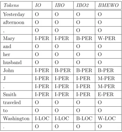
Tagging Scheme There are several types of tagging scheme that both datasets and models have to follow. Table 1 shows examples of different tagging schemes. IO scheme is the simplest and most straightforward scheme. It tags tokens either as “I” only if they appear inside of a name or “O” only if they are not. However, when it comes to further processing, the lack of border between two different names will make it difficult to separate. IBOand IBO2 tag the beginning name token as “B”. The only difference between these two schemes is that IBO2 tags any beginning name token as “B”, while IBO tags a token “B” only if this token is followed by a token from the same name. A name token which is surrounded by “O” tokens will still be tagged “I”. As illustrated in Table 1, “Mary” and “Washington” are tagged differently according to IBO and IBO2. BMEWOfurther distinguish entity borders besides beginning border “B” tag. It will tag the middle tokens of an entity as “M” and the ending token of an entity as “E”. For entities of a single token, they will be tagged as W. In my thesis, IBO2 tag is used for its simplicity.

(13)

Tokens IO IBO IBO2 BMEWO

Yesterday O O O O

afternoon O O O O

, O O O O

Mary I-PER I-PER B-PER W-PER

and O O O O

her O O O O

husband O O O O

John I-PER B-PER B-PER B-PER

J I-PER I-PER I-PER M-PER

. I-PER I-PER I-PER M-PER

Smith I-PER I-PER I-PER E-PER

traveled O O O O

to O O O O

Washington I-LOC I-LOC B-LOC W-LOC

. O O O O

Table 1: NER tagging scheme

3.3.2 NER Model

In this part, the goal is to implement and evaluate a Finnish NER model as a part of my Proj-NER. The NER model and its setup are inspired by the models introduced and evaluated by Ma and Hovy [31] and Reimers and Gurevych [37]. My model is modified from the original BiLSTM-CNN-CRF model, which is proposed by Ma and Hovy [31]. Compared to the feature mentioned in the original articles, PoS information is utilized as one additional input features. Hopefully, it can improve the performance of the model.

Manual checking is conducted to evaluate the true performance of the NER model after training. Besides regular model performance evaluation, the quality of differ-ent English NER taggers, such as rule-based NER tagger or neural network based NER tagger, and their influence on the performance of Proj-NER is a part of the evaluation as well.

(14)

3.3.3 Locality Resolution

In this part, the goal is to resolve all the location names and assign each article the most salient location.

After resolving all the named entities of an article, the metric salience is used to select the most important location name as the locality of an article. Articles are plotted on a map as visualization according to their locality. A location-coordinate dictionary is used for obtaining the coordinate of a geo-location.

3.3.4 Named Entities in Document Representation

The goal of this experiment is to answer one question: Does the representation of named entities contribute to the quality of document representation?

The same indirect evaluation method used by Chen [9] is adopted, which is to solve a document classification task. By comparing the performance of document representations with different named entity setups, researchers can get a better understanding of the role of named entities in document representation and how to handle them to achieve better performance.

3.4

Neural Network

I will give a brief introduction to three typical neural networks: MLP, CNN, and RNN.

The idea of neural networks is inspired by the way how the brain works. It is a framework instead of a single algorithm as other machine learning approaches. One example is multi-layer perceptron (MLP). It is one of the most fundamental types of neural network. Such networks have an input layer, an output layer, and several hidden layers. Each layer has several nodes (neurons). Each neuron takes a weighted sum of the outputs from its previous layer and passes it to its next layer after applying an activation function. Examples of activation functions are sigmoid (σ(x)) and tanh(x).

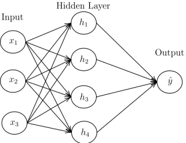
Figure 2 is a simple example of MLP with only one hidden layer. A single hidden layer network can be formalized as yˆ = g(V h(W x)). W and V are two weight matrices, h(·) and g(·)are two activation functions.

(15)

Input Hidden Layer Output x1 x2 x3 h1 h2 h3 h4 ˆ y

Figure 2: An example of MLP network

for each layer. The objective function in the training—the loss—is the difference between y and yˆ, where y is the ground truth and yˆ is the output of the MLP. Essentially, back-propagation computes gradients on each neuron with respect to later neurons using the chain rule. Because of the chain rule, the loss is distributed across the whole network. Back-propagation adjusts the weights of all neurons in a network so that the loss can be reduced.

Convolutional Neural Network(CNN) utilizes convolution as a part of a network and obtains the information of the local neighbourhood of each neuron. CNN is therefore capable of solving tasks like image recognition.

Convolution on 1-dimensional space can be discretely formalized as (f ∗g)(t) = P

mf(t−m)g(m). Function f(·) refers to an input, while function g(·) refers to a

kernel function. The output of a convolution is referred as a feature map. Convolu-tion can be extended to 2-dimensional space or more.

Besides convolution layer, CNN introduces two pooling layers: max pooling and average pooling. They scan over the feature map produced by the previous layer and extract max or average values of each neighbourhood.

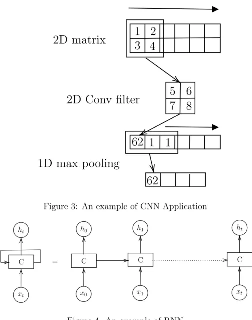
Figure 3 is one example of CNN. A 2D Conv filter of size 2×2 and stride 1 scans over a 2D matrix and outputs a 1D feature map. A 1D max pooling layer of stride 1 extracts the maximum value of each neighbourhood.

Although the output of the example shown in Figure 3 is of 1D and ready to be sent into 1D feed-forward layers, there will usually be an additional layer between

(16)

1

4

2

3

5

6

7

8

62 1 1

62

2D matrix

2D Conv filter

1D max pooling

Figure 3: An example of CNN Application

C xt ht C x0 h0 C x1 h1 C xt ht = Figure 4: An example of RNN

a Conv layer and a 1D feed-forward layer to flatten multi-dimensional feature map into a 1D array.

MLP and CNN are considered as feed-forward networks. Recurrent Neural Net-work (RNN) utilizes recurrent links, which allows the output of each neuron to be linked back from the previous time step. Because of this feature, RNN can be applied for tasks such as sequence tagging.

Figure 4 is a simple illustration of RNN. The left side of Figure 4 shows how recurrent link connects RNN cell back to itself after computing the “cell state” (hidden state). The right side illustrates how the recurrent connection passes information over time. Here,xtrefers to the input, htrefers to the output with respect to the corresponding

(17)

+ σ σ tanh σ tanh Ct−1 Ct ht−1 ht ht xt ft it ot × × ×

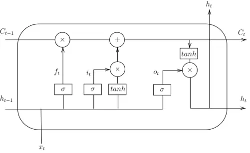
Figure 5: An example of LSTM unit

There is a problem which comes along with fitting through a sequence: vanish-ing gradient. The gradients may be close to zero or explode after fittvanish-ing with a long sequence. To solve this problem, researchers have proposed several RNN cell structures. One of them is Long Short-Term Memory (LSTM).

As shown in Figure 5, an LSTM unit is an RNN cell which is composed of a forget gate, an input gate, and an output gate. They can be formalized as follows:

• Forget gate: ft=σ(Ufxt+Wfht−1)

• Input gate: it=σ(Uixt+Wiht−1)

• Output gate: ot =σ(Uoxt+Woht−1)

• MatricesU and W are weights of xt and ht−1 for different gates

In Figure 5,Ct andCt−1 refer to the cell state, where Ct−1 can be updated to Ct by

applying the input and forget gates: Ct =ft×Ct−1+it×tanh(Ucxt+Wcht−1), where

Wc and Uc are another pair of weight matrices. The symbol × refers to

element-wise vector multiplication. The output of the cell will be filtered by output gate:

ht=ot×tanh(Ct). The idea of “forgetting” is to decide what information should be

thrown away. With the help of “forgetting”, vanishing gradient problem is solved.4

4_{Figure 4, Figure 5 and gate formulas are inspired by the online blog post}

https://colah. github.io/posts/2015-08-Understanding-LSTMs/

(18)

LSTM LSTM LSTM LSTM

xt−2 xt−1 xt xt+1

ht−2 ht−1 ht ht+1

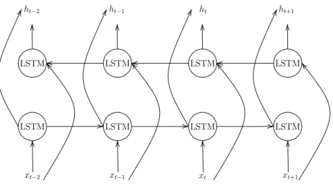
Figure 6: The structure of BiLSTM

Another problem in RNN is that a regular RNN network runs only in one direction, which is usually chronological direction. This works well for single-directional data, such as heart rate sequence. But what about the bi-directional data? For a text sequence, information of different parts of the sequence can be inter-connected from both forward and backward directions.

To solve this problem, Bi-direction LSTM (BiLSTM) is proposed on the basis of LSTM. The idea of BiLSTM is to utilize two LSTM layers for forward and backward directions of a sequence and concatenate the outputs of two LSTM layers. Figure 6 is a diagram of BiLSTM.

3.5

Word Embedding

Word embedding is one type of representation of document vocabulary. It has now been implemented in many NLP applications. Compared to other statistical lan-guage models (SLM), such as N-gram, word embedding will not learn the probability distribution of words in different contexts but the vector representation of each word. Several word embedding approaches will be briefly discussed in this subsection.

One way of obtaining an embedding is to use a neural network. Google’s Word2Vec [32] is one well-known example. There are two architectures for training a Word2Vec embedding. As shown in Figure 7, both of them contain one input layer, one hidden layer, and one output layer, and the training process is unsupervised. The CBOW model will take the surrounding context of word w(t) as input and try to predict

(19)

Figure 7: Neural Networks for Word2Vec [32]

w(t).

Word2Vec covers only word-level embeddings, which leads to its poor performance for morphologically-rich languages. Such languages make extensive use of prefixes, suffixes and compound words. One base form may be inflected to many surface forms. Therefore, it is impossible to have enough data to train a good embedding for the surface forms.

To solve this shortcoming, Facebook’s Fasttext [8] is proposed. It is built on an idea similar to Word2Vec, but it uses all substrings of a word. For example, the word “disagree” and its substrings “dis”, “isa”, “sag”, “agr”, “gre”, and “ree” are all included in Fasttext training process. This approach leads to better support for morphologically-rich languages and solves the out-of-vocabulary problem. However, this also suggests that Fasttext needs more memory allocation and computational power in training and actual usage, compared to Word2Vec.

GloVe [35] takes a different approach to word embedding, which is statistical. It first builds a word-word co-occurrence matrix and defined an approximate equation between the co-occurrence probability of words wi and wj and their word vectors.

(20)

other conditions. By optimizing a weighted loss function, the word representation is obtained. Similarly to Word2Vec, GloVe takes advantage of the local context window. However, GloVe also takes global corpus information into consideration through the word-word co-occurrence matrix, while Word2Vec and Fasttext do not [35].

Researchers have also proposed more advanced word embeddings. ELMo [36] and Flair [1] are two examples. Both are implemented on the basis of BiLSTM. ELMo is still a word-level embedding, while Flair is based on the concatenation of character-level embedding. Compared to Word2Vec, Fasttext and GloVe, ELMo and Flair produce context-specific word embeddings. A token may be assigned with different embedding according to its context. This is an advantage for disambiguation. But on the other hand, utilizing BiLSTM leads to a more time-consuming and memory-intensive training process.

One of the goals and benefits of word representation is to measure the similarity of words. For example, “hound” and “dog” should be close to each other. Another benefit of applying embeddings is that it can help to obtain analogy. In Word2Vec, the most similar word tovec(”king”)−vec(”man”)+vec(”woman”)isvec(”queen”). For the task of NER, the quality of embedding is essential. The better the word embedding, the better the result will be [37, 36, 1]. However, due to the fact that ELMo and Flair are very time-consuming and memory-intensive, only Word2Vec and GloVe will be used in my thesis.

3.6

Document Representation

Similarly to word representation, document representation, also referred as docu-ment embedding, maps a docudocu-ment to an n-dimensional vector. It is concerned about how text should be represented in different problems, such as topic classifica-tion and measuring the similarity of documents.

One approach to build document representation is to use a weighted average of the word embeddings. The weight of a word embedding can either be the frequency of its corresponding word in an article, or the inverse document frequency (IDF) with respect to a corpus. Each dimension of this document embedding can be regarded as a summary of the same dimension of the word embeddings. As a whole, a document embedding, therefore, summarizes its corresponding document.

(21)

Figure 8: The framework of learning Doc2VecC [9]

introduces two models: Distributed Memory Model of Paragraph Vectors (PV-DM) and Distributed Bag of Words version of Paragraph Vectors (PV-DBOW). PV-DM takes the surrounding context tokens and an additional paragraph vector as an input and predicts the center word, while PV-DBOW takes only paragraph vector and predicts context tokens. Both models are initialized randomly and train paragraph vectors directly. Others have also proposed indirect approaches, where a paragraph embedding is assembled with certain rules. Huang et al. [23] improve the PV-DM model by utilizing globally averaged word embeddings as the paragraph vector. Although the goal is to improve the quality of word embeddings by introducing both local context and global context into training, the paragraph embedding will benefit from this approach as well. Similarly, in Doc2VecC [9], the paragraph embedding is assembled via averaging word embeddings of randomly sampled words from a document. Despite the “corrupted” document representation due to dropping a significant portion of words, this model outperforms other approaches in several tests. Figure 8 is an illustration of training a Doc2VecC model.

3.7

Conditional Random Field

Conditional Random Field (CRF) is a discriminative probabilistic model. One sta-tistical approach for NER, Stanford NER, is built on CRF and has been proved to be effective in many different languages [18].

(22)

con-y0 y1 y2 y3 x1 x2 x3 ... ... _y 0 y1 y2 y3 x1 x2 x3 ... ...

Figure 9: HMM and Linear CRF [40]

cept and application will be introduced here, especially in the NER scenario.5

Structurally, linear CRF model is very similar to Hidden Markov Model (HMM), but HMM is a Directed Acyclic Graph (DAG), while CRF is undirected. Figure 9 illustrates the structure of HMM and linear CRF. For both models, the shaded nodes are the hidden state variables and the light nodes represent the observed variables. For HMM, an observed variable depends on its corresponding hidden variable, while a hidden variable depends on its previous hidden variable. Using the chain rule, the joint probability of HMM can be decomposed as follows:

P(X, Y) =P(y0) T−1 Y t=1 P(yt+1|yt) T Y t=1 P(xt|yt) (8)

In (8), y0 refers to the initial state probability, P(yt+1|yt) is state transition

proba-bilities and P(xt|yt) is emission probabilities.

Linear CRF is a discriminative case of HMM. In Linear CRF, an observed variable has a connection with its corresponding hidden variable, while a hidden variable also has connections with both its previous and later hidden variables. Lafferty et al. [27] formulate the conditional probability as:

P(Y|X) = 1 Z(X,Θ)exp X t X k θkfk(yt, yt−1, xt) , (9) where Z(X,Θ) =P yexp( P t P kθkfk(yt, yt−1, xt))

In this equation,fkrefers to feature function andθkis the parameter with respect to

featurek. In practice, one uses not only a single feature as input but also features like suffix, prefix, PoS and other character-based features to improve the performance of the model. Therefore, there may be more than one value of k in the summation in (9).

5_{The CRF sequence model that is discussed here and Stanford NER are linear CRF rather than}

(23)

B-ORG O B-MISC O

EU rejects German call

O

.

Figure 10: An example of CRF model for NER

An efficient inference algorithm for CRF is critical during the training and predicting process. For linear CRF, the algorithms are very similar to the inference algorithms for HMM: the forward-backward algorithm and the Viterbi algorithm.

The forward-backward algorithm computes the posterior marginal probabilities for all hidden variables given the observations from both forward and backward direc-tions.

The Viterbi algorithm assigns the most likely states to hidden variables for prediction based on the result of the forward-backward algorithm. It is a dynamic programming algorithm, and its recursive equation can be obtained by utilizing part of the outcome from the forward-backward algorithm.

Detailed mathematical explanations for these two algorithms can be found in the work of Sutton et al. [40] or other textbooks. With further specifications, these algorithms can be used for linear CRF.

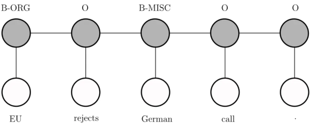
In practice, linear CRF can be utilized in many different fields including NLP, com-puter vision and bioinformatics. In NER, a sequence of tokens is the input data. The features of each token, such as PoS, and other semantic roles, can be fed into the model as well. Figure 10 shows an example of how CRF models a sequence of tokens and labels them for NER.

3.8

Bi-directional LSTM

Bi-directional LSTM (BiLSTM) is another tool for sequence modeling. Chiu and Nichols [10] proposed a BiLSTM model with multiple input features to solve the task of NER. In this subsection, I introduce this BiLSTM NER model.

(24)

J O H N Padding Padding Charater Embeddings Charater Feature Map Conv 1D Max Pooling Character Information

Figure 11: The extraction of character information with Conv

As introduced previously, BiLSTM can extract information from both the forward and the backward direction, which allows it to model a text sequence, since each token may have a connection with its surrounding tokens. As shown in Figure 6, in the case of NER, xn is the embedding vector of a certain word, and hn is a feature

vector that is fed into the output layer. Eventually, each token is annotated.

Chiu and Nichols [10] feed a concatenation of four features as the input to their BiLSTM NER model: word representation, character representation, case feature and lexicon feature.

Character representation is introduced to extract the suffix and prefix information of a word. To achieve this goal, character embeddings are randomly initialized. As shown in Figure 11, they pass through the Convolutional layer and 1D Max Pooling to extract the character information.

Case feature can be as follows:

• Fully capitalized token, such as: “USA”, “NASA”

• Tokens with only the initial letter capitalized, such as: “Donald” • Fully lower case token

(25)

J O H N Padding Padding Charater Embeddings BiLSTM Character Information LSTMs LSTMs LSTMs LSTMs k

Figure 12: The extraction of character information with BiLSTM

• Tokens with mixed uppercase and lowercase, such as: “al-Qaeda” • Punctuation token

• Other

Case feature is encoded in a similar way as embedding and transformed into a vector through a Look-up table. The table can be trained with back-propagation too [11]. After vectors are transformed, they can be fed into the Conv layer and the Max Pooling layer. The resulting feature map is used for further processing.

Lexicon feature is constructed by Chiu and Nichols [10] from a list of known named entities in DBpedia [3] on the basis of the categories defined in CoNLL-2003 NER shared task.

According to Chiu and Nichols [10], the contextualized input with additional infor-mation outperforms not only the regular feed-forward neural network but also the BiLSTM with only word embeddings.

(26)

3.9

BiLSTM-CRF

BiLSTM and CRF have been proved been effective on the task of NER. What about a hybrid model combining both models? Ma and Hovy [31] and Lample et al. [29] have proposed two models with BiLSTM layers and CRF output layer. Both of them contain character information as a feature. In the model of Ma and Hovy [31], character information is obtained in the same way as Chiu and Nichols [10], while in the model of Lample et al. [29], it is obtained by BiLSTM. Figure 12 shows the architecture of the neural network to obtain the character information.6

Additionally, the model of Ma and Hovy [31] applies case information as a feature, while the model of Lample et al. [29] does not. All the features are concatenated and fed into BiLSTM layers. Eventually, the output is obtained by decoding the result of the CRF layer.7

Reimers and Gurevych [37] evaluate the performance of the models proposed by Ma and Hovy [31] and Lample et al. [29] with a different parameter setup. They claim that the model proposed by Ma and Hovy [31] can be trained within much less time than the model proposed by Lample et al. [29], while their performance is comparable. Therefore, my master’s thesis is inspired by Ma and Hovy [31] and mostly follows its implementation. Figure 13 shows the general network structure.

All the word embeddings used by Lample et al. [29], Ma and Hovy [31] and Reimers and Gurevych [37] are context-independent, such as Word2Vec, which only map a token to a unique embedding vector. Peters et al. [36] include ELMo embedding, which is context-dependent, as an additional feature and feed enhanced embedding into BiLSTM-CRF. Akbik et al. [1] uses only the Flair embedding as the input for BiLSTM-CRF after concatenating the character-level embeddings for each token.

Figure 14 is a diagram modified on the basis of Akbik et al. [1] to show the structure of Flair-BiLSTM-CRF.8 BiLSTM-CRF with context-independent embedding, such as Word2Vec, can get access to the information only within the scope of context (a sentence). With Flair, global information about the entire article is implicitly included.

6_{The symbol}_k_{refers to the concatenation of input vectors in this thesis.}

7_{Reimers and Gurevych [37] also include}_{numeric case} _{as one type of case information.} 8_{Character language model refers to Flair here.}

(27)

Figure 13: BiLSTM-CRF network structure [37]

3.10

NER by Pattern Mining

In addition to the probabilistic approaches and the neural network based approaches for NER, pattern mining can also be used as an approach for NER. It assigns the type of a named entity based on patterns of phrases. For example, for a sentence: “Presidential candidate x visited y last month”, we can infer that named entityx is a person, and y is a location.

In PULS [16], a domain-specific pattern-based approach is used. Although the goal of the pattern mining here is to learn the event described by a sentence, it can also be utilized for NER.

Du et al. [16] first used an Apriori-like algorithm [6] to find raw patterns of high frequency. The frequency of a pattern is obtained in the following step:

1. Remove stop words and punctuation.

2. Replace names with their type. Du et al. [16] used a name dictionary and another existing NER module to obtain the data for further pattern mining.

3. Represent a sentence as a transaction T of hW1, W2, W3, ..., Wni.

4. For a transaction hW1, W2, W3i, only sequential patterns are allowed, namely hW1, W2i, hW2, W3i orhW1, W2, W3i. Pattern hW1, W3i is not allowed.

(28)

D o n a l d T r u m p e l e c t e d . vecT rump Character Language Model Sequence Tagging I-PER

Figure 14: Flair-BiLSTM-CRF network structure

5. The candidate count |P| will increase if pattern P can be found in different

transaction.

6. The support Sp =|P|/|T|, where|T|is the number of transactions.

The idea is to keep frequent patterns only (Sp ≥ Smin, where Smin is a threshold).

The frequent patterns are then manually filtered according to validity and scenario.

3.11

Pre-processing Components for NLP

Although NER approaches are essential to this thesis, pre-processing is also of great importance for my project. At the end of this section, I will introduce some key components that are used for pre-processing.

The raw input data for most NLP systems are unstructured text strings, such as articles that we can read in a book or newspaper. A pre-processing pipeline trans-forms the raw data to add some structure to it, so that the data can be further analyzed. There are three key components in the pipeline: tokenizer, syntactic parserand morphological analyzer. Their functions are listed as follows:

• A tokenizer breaks a sentence into tokens.

• A syntactic parser parses the relationship of each token based on lexicon in-formation and assigns each token its grammatical role. It also splits sentences.

• A morphological analyzer takes the surface form of a token as input and out-puts its base form, PoS, tense and other grammatical features.

(29)

For English, the tokenizer, syntactic parser and morphological analyzer are well-studied. Many are freely available, such as NLTK.9 For my project, the integrated pre-processing pipeline in PULS project [16] is used.

For Finnish, our tokenizer and syntactic parser are the Turku Dependency Tree-bank [21], which contains more than 200,000 tokens from 10 text sources. Inter-nally, the dependency treebank is based on the well-known Stanford dependency scheme [13] and a statistical dependency parser [7]. For the sentence “Sen odote-taan olevan 0,69 euroa osaketta kohti.”, here is one simplified output example of the parser:

Sen se PRON Case=Gen|Number=Sing|... 2 dobj

odotetaan odottaa VERB Mood=Ind|Tense=Pres|... 0 root

olevan olla VERB Case=Gen|Degree=Pos|... 2 xcomp:ds

0 0 NUM NumType=Card 7 nummod

, , PUNCT _ 4 punct

69 69 NUM NumType=Card 4 conj

euroa euro NOUN Case=Par|Number=Sing 8 nmod

osaketta osake NOUN Case=Par|Number=Sing 3 nmod

kohti kohti ADP AdpType=Post 8 case

. . PUNCT _ 2 punct

Though the direct output of this Finnish dependency parser is hard to read, it is noticeable that the parser tokenizes and extracts a syntactic tree from the sentence as indicated by the numbers of the second last column. The parser we use outputs PoS and lemma of each token as well. However, we do not use this information, because this parser may sometimes give wrong partitioning for compound words due to ambiguity. Since it gives only one resolution for each token rather than all possible candidates, it is difficult to disambiguate based on the output of the parser.

To get a full analysis for each token, a Finnish morphological analyzer is therefore applied in my thesis. This analyzer is a combination of morphological lexicon and a loss-less hyper-minimization algorithm [15, 33]. Here is one example output of our Finnish morphological analyzer:

[Finnish-analyser]> valtakirjassa

{’analyses’: {’Finnish’: [[{’base’: ’valtakirja’,

9

(30)

’pos’: ’Noun’,

’tags’: {’CASE’: ’Nom’, ’NUMBER’: ’Sg’}}], [{’base’: ’valta’,

’canon’: ’valta+kirja’, ’pos’: ’Noun’,

’tags’: {’CASE’: ’Nom’, ’NUMBER’: ’Sg’}}, {’base’: ’kirja’,

’tags’: {’CASE’: ’Nom’, ’NUMBER’: ’Sg’}}], [{’base’: ’valta’,

’canon’: ’valta+kirja’, ’pos’: ’Noun’,

’tags’: {’UNKNOWN’: [’Pref’]}}, {’base’: ’kirja’,

’tags’: {’CASE’: ’Nom’,

’NUMBER’: ’Sg’}}]]}, ’surface’: ’valtakirjassa’}

As demonstrated in this example, the Finnish morphological analyzer not only gives the PoS information and the lemma of the word ’valtakirjassa’, but also finds all possible partitionings for this compound word. In Finnish, the last part of a lemma has the main influence on the meaning and PoS of a word. Therefore, if this word is out-of-vocabulary, we can utilize the word embedding and PoS of its last part as compensation.

4

Automatic Annotation Pipeline

In this section, I discuss my automatic annotation pipeline. The idea of this pipeline is to use English named entities, annotated by an existing English NER tagger, as the source of annotation and project the types of the named entities from English to Finnish. This projection is done by resolving and matching the base forms of named entities.

(31)

4.1

Raw Data Source

English news gathering English news are collected by PULS system [16] from over 3,000 sources. Over 5,000 documents are gathered daily.10

Finnish news gathering Finnish news are collected from Helsingin Sanomat and Yle. Around 200 documents are collected every day.11

4.2

Name Pre-processing

English text processing Each document collected by the system is processed by a cascade of pre-processing classifiers, including a pattern-based named entity tagger. Here, the base forms of names and their types are obtained, which are later used for projection.

The performance, especially the precision, of the English NER tagger is therefore crucial for the entire pipeline. It is worth pointing out that the precision of the English NER tagger controls the quality of the projected Finnish data. The recall, on the other hand, determines the variety of the projected named entities. Lower recall rate can be compensated by feeding in more news articles. Therefore, in this thesis, the precision of the English NER taggers is considered to be more essential than the recall or the overall F1 score.

For comparison, I also trained two BiLSTM-CRF models [31, 29, 37] from scratch, using Word2Vec and GloVe word embeddings. These models were trained on the CoNLL2003 English dataset. Table 2 shows an evaluation of all three English NER taggers on the CoNLL2003 test dataset

As illustrated in Table 2, BiLSTM-CRF English NER taggers that trained with CoNLL2003 have a high f-score. However, the results are different from what was reported in the papers of Ma and Hovy [31], Reimers and Gurevych [37], since I used a default hyper-parameter setup, rather than using the fine-tuned setup in the papers.

The PULS NER tagger has a worse performance if compared to BiLSTM-CRF English NER taggers. I should mention that the PULS NLP system has different tokenization compared to the CoNLL dataset, and our pattern-based NER tagger

10

http://newsweb.cs.helsinki.fi/

(32)

Source prec rec F1

PULS 0.68 0.37 0.30

BiLSTM-CRF-GloVe 0.87 0.85 0.85 BiLSTM-CRF-W2V 0.89 0.90 0.89

Table 2: The quality of English NER taggers on ConLL2003 test dataset. “PULS” refers to the PULS pattern-based English NER tagger, while “BiLSTM-CRF-GloVe” and “BiLSTM-CRF-W2V” refer to the BiLSTM-CRF model trained with Glove and Word2Vec respectively.

is customized for the business news domain. Though the output of our pattern-based tagger is aligned to be comparable with the CoNLL dataset, the content of its test dataset, which is mostly sports news, is still skewed against our tagger. In practice, our tagger achieves higher precision on business news. To confirm this, I evaluate the PULS tagger on 10 randomly selected articles, containing both general and business news. Although this is a simple experiment, the overall precision of the PULS tagger increases to 77%.

Finnish text pre-processing The Turku dependency parser [21] has been ap-plied for sentence splitting and tokenization. Three different problems need to be solved so that all potential names can be extracted in these steps: name identifica-tion, base form selecidentifica-tion, and name merging.

Name identification For identifying whether a token is a name or part of a name, I use the rules based on the position of tokens as follows:

• Any capitalized token which appears in the middle of a sentence is definitely a name or part of the name.

• If token A is a name according to the previous rule, and token B, having the same base form as token A, appears at the beginning of a sentence, I assume token B is the same name.

• If a token of a potential name appears in the document only at the beginning of sentences, it is not certain and therefore not assumed to be a name.

Base form selection To determine the base form corresponding to a surface form found in a text, I consider all base forms returned by our morphological analyzer [33],

(33)

and a simple rule-based stemmer, and look through the entire article. If there is an intersection between the possible base forms of two name tokens, their true base form can then be resolved. When the intersection has only one base form, it can be confirmed to be the base form of a name directly. Otherwise, all of them will be recorded as potential base forms of the name. All potential base forms will be further filtered when matching with English named entities during projection.

Suppose the surface form “Trumpille” (in the allative case) and “Trump” (nomina-tive) both exist in an article. Without any external knowledge, the Finnish surface form “Trumpille” will be assigned two potential lemmas by our stemmer: “Trumpi” and “Trump” (both of these lemmas have the same allative form). For the sur-face form “Trump”, only “Trump” will be returned as a potential lemma. Then, in this case, their intersection, “Trump”, will be confirmed to be the lemma of both “Trumpille” and “Trump”. However, if instead the article only contains the sur-face forms “Trumpille” and “Trumpin” (genitive). Then both lemmas “Trumpi” and “Trump” will be recorded as potential lemmas.

We perform name identification and base form selection jointly, since they are con-nected, by searching for the common base forms of tokens.

Name merging I use a set of rules to merge names that consist of more than one token. Potential names can contain only the following kinds of tokens in positions other than the final position:

• Singular common noun or proper noun which must be in the nominative case, for example: “Spring Harbour”.12

• English function words: e.g., “the”, “and”, “new”, etc. For example: “The New York Times”

• Having no valid analyses returned by the Finnish morphological analyzer, and its surface form can be confirmed to be its own lemma during the base form selection process above.

One example is the token “Trump” in “Trump Towerin” (genitive: “of the Trump Tower”). Our Finnish morphological analyzer will reject (not recognize) the input token “Trump”. I assume that “Trump” can be confirmed as a name or as part of a multi-token name according to the rules. “Trump” can be

12_{Names such as “Helsingin Sanomat” (name of a major newspaper in Finland), where the first}

token is in thegenitivecase (of “Helsinki”) are currently not handled by these rules, and are handled separately by a list.

(34)

confirmed to be its own base form, which means its base form happens to be the same as its surface form. In this case, “Trump” will be merged with the following token “Towerin”.

We should note that when several potential name tokens are strung together, the true partitioning of names is ambiguous. During name merging, all different partitionings and potential forms of the base forms of names are cached as candidates for the following name resolution step.

Hyphenating between tokens is also a criterion for merging names, such as the Indian surname “Ankalikar-Tikekar”.

4.3

Name Projection

In the next stage, I annotate Finnish names by utilizing the potential names candi-dates produced by the previous three steps, namely name identification, base form selection, and name merging.

The fundamental assumption is that a name refers to only one entity in a given article (The “One Sense Per Discourse” Assumption [43]). This assumption is ex-pected to hold for well-edited news articles. This means that if only one instance (surface form) of a particular name has been annotated in an article, the remain-ing occurrences of the same name in the article—possibly involvremain-ing other surface forms—can be annotated as well.

Two sets of named entities are gathered from Finnish document and English docu-ments:

• For a Finnish document, published on day t, the previous three steps, name identification, base form selection and name merging, are used to obtain a set of potential Finnish named entity candidates, including both potential base forms and confirmed base form of names.

• From English news in the time interval (t±2 days), using an English NER tagger, a set of English named entities and their corresponding tags are ob-tained. Each of them has its base form resolved by the pre-processing pipeline in PULS.

Names can naturally be matched according to their base form. The type of the English named entities can, therefore, be projected to their Finnish counterparts.

(35)

The remaining Finnish names candidates, for which no type annotation can be inferred, are dropped after this step.

The idea of a time window (t±2days) is to take advantage of the fact that names overlap significantly in different articles due to continuous coverage of important events, and therefore optimize the memory usage and time efficiency.

Again, take “Trump” as an example. Suppose I have a named entity “Donald Trump” from the English news articles and it is recognized as “Person”. I may have “Donald Trumpille” in a Finnish article; if the surface form “Trump” is not present in the same Finnish article, as I mentioned already, I can only infer that the base form of “Trumpille” is “Trumpi” or “Trump”, using stemming rules. In addition, “Donald Trumpille” has two tokens but I do not yet know whether they belong together as one name. Therefore, “Donald”, “Donald Trump”, “Donald Trumpi”, “Trump” and “Trumpi” are all Finnish name candidates. After matching, only “Donald Trump” will be kept and annotated as Person, while other candidates, namely “Donald”, “Donald Trumpi”, “Trump” and “Trumpi”, are dropped.

In addition, for the Person type only, names are connected by their partial base form. Once “Donald Trump” gets annotated, all the other “Donald” and “Trump” tokens in the entire article will be annotated as Person as well.

4.4

Special cases: rule-based projection

I use extra steps to handle special cases in this process. In Finnish, geo-location names, such as the names of countries, are often different from their English names. For example, France is “Ranska” in Finnish, and the United States is “Yhdysval-lat” in Finnish. Some organizations also have the same problem, as UN is “YK” in Finnish, etc. Therefore, I manually build a small database of frequent names, including Finnish geo-locations, and a few of the major and most frequently occur-ring international companies and organizations, to assure that they are annotated correctly. In addition, this covers some cases which the English tagger fails to catch. I also filter out names that can have multiple types, such as MacLaren, since these are ambiguous.

Additionally, I introduce a list of 1000 common first names and assume that names beginning with these tokens are of type Person. However, this practice requires more rules to constrain its outcome:

(36)

• A Person name should have at most 2 tokens. • A Person name should not start with “The”.

• No token in a Person name should be fully uppercase.

• A Person name should be mentioned using the full name at least once in the article.

These rules are simple, naive and strict. The purpose of these rules is to remove any uncertain instances and make the data as clean as possible. Even if only one name in an article can meet all these rules, all other name instances related to that name instance will be correctly annotated. Also, taking advantage of our enormous amount of data, I can afford to filter out uncertain data without worrying about the amount of remaining data.

Currently, the annotations may be wrong when an article only mentions the last name of a person, which also happens to be the name of a location. For example, “Sipilä” is the last name of the former Prime Minister of Finland, and may, therefore, be mentioned many times in an article, without mentioning the full name, “Juha Sipilä”. Coincidentally, “Sipilä” is a town in Finland. The situation where both the person and the location are mentioned in the same article rarely occurs in practice and can be tackled by filtering out such names.

5

NER Model

In this section, the details of the adapted BiLSTM-CRF model for Proj-NER and the hyperparameter setup for training this model are introduced. The basic network structure of the model is inspired by [31, 37]. The model is implemented in Keras with TensorFlow as its backend. The CRF layer is provided by Keras-contrib13. The training process runs on an Nvidia GeForce 1080 Ti GPU. It took around 3 hours to train the model using the setup in this section. The model is shown in Figure 15.

As seen in Figure 15, Part-of-Speech (PoS) is included as an additional feature, com-pared to the model of [31]. This is because a lemma may be assigned multiple PoS tags by our morphological analyzer [33]. Word embeddings such as Word2Vec [32] may implicitly contain PoS information but will still be static regardless of context.

(37)

Tag 0 CRF Linear BiLSTM Tag 1 CRF Linear BiLSTM Tag 2 CRF Linear BiLSTM Word Emb. Char CNN Case Emb. PoS k PoS-dense Token 1 CRF output layer Linear layer BiLSTM layer ... ... ... ...

Figure 15: Adapted BiLSTM-CRF network structure for Proj-NER

Using PoS as an input feature also compensates for the out-of-vocabulary problem in embeddings. In these cases, not even the implicit PoS information can be detected by the network if PoS is not a part of input features.

5.1

Data Encoding

Tokens are encoded into to several features: word embedding, character embedding,

case embeddingandPart of Speech(PoS). Except for PoS, most of the features follow the setup in [37]. Word embeddings are extended with a special mark for ambigu-ous tokens—tokens, for which our morphological analyzer fails to return more than one base forms and PoS. These tokens are replaced with a special token “AMBIGU-OUS”. Additionally, I only use the embedding of the last part of a compound word if this word is out-of-vocabulary. This is because the last part is the essential part of compounds in Finnish. Character embeddings are extended with a special value for “unrecognized” character. The PoS feature is encoded as an array of ones and zeros. Each dimension corresponds to one PoS type, including PADDING and UN-KNOWN. Integer “1” is assigned to the dimension corresponding to the token’s PoS. If a token is a compound word, only the PoS of its last part is used for encoding. If a token has multiple PoS analyses, more than one position in the PoS array is assigned “1”. The values of PoS are as follows:

(38)

• PADDING • UNKNOWN • Noun • Verb • Adj • Adv • Pron • Conj • Interj • Num • Punct • other

5.2

Parameter Initialization

Word Embedding I am using a pre-trained Word2Vec embedding matrix trained by [28]. It has been trained on 4.5B words. As mentioned previously, vectors for “PADDING”, “UNKNOWN” and “AMBIGUOUS” tokens are included. Both “UNKNOWN” and “AMBIGUOUS” tokens are randomly initialized with the uniform sampling from -0.25 to 0.25, while “PADDING” embedding is a zero vector.

Character embedding Character embeddings, including “UNKNOWN” charac-ter embedding, are randomly initialized with uniform samples from−» 3

dim to »

3

dim,

where dim= 30.

Case embedding Case embeddings are randomly initialized using the Keras de-faults, which is applying a uniform initializer. And the dimensionality of the case embeddings is 10.

Weight Matrices and Bias Vectors Weights and bias of the network follow the default setup in Keras. Most of the weights are initialized as an uniform sample from[−» 6

Ni+No,

» ₆

Ni+No], whereNi andNo refer to the number of input and output units in weight tensor respectively. Bias is initialized with zeros.

5.3

Optimization

Optimizer I used the Adam optimizer, as recommended in [37]. The setup for the Adam optimizer also followed the Keras default setting: lr = 0.001, β1 = 0.9, β2 =

(39)

Early stopping and learning rate decay I applied early stopping following the categorical accuracy on the training dataset in case of over-fitting. On average, the training process stops after 5 epochs. I have also explored reducing the learning rate during the training process if the accuracy stops improving. However, this made the training slower, and did not improve the final result on the validation dataset.

5.4

Hyper-parameter Setup

Most of hyper-parameters values, shown in Table 3, follow the recommendations in [37]. The layer called “PoS-dense” in Figure 15 is a dense layer with a non-linear activation function, rather than an embedding layer, due to the encoding method of the PoS features, as explained in Section 5.1. For the mini-batch size, the authors recommend using the batch size between 8 and 32, depending on the size of the training dataset. However, that is the result on the CoNLL-2003 dataset, which is an English dataset. I use 50 similarly to the German NER model in [37].

I should mention that the CRF layer implemented by the Keras-contrib pack-age offers two different modes for the training and testing processes: “Join” and “Marginal” for training, “Viterbi” and “Marginal” for testing. The “Join” training mode and “Viterbi” testing mode follows the “vanilla” fitting algorithms for lin-ear CRF. “Marginal” training is optimized via composition likelihood (product of marginal likelihood), which is not optimal in this case. “Marginal” testing mode will decode the input sequence according to the training result and compute marginal probabilities. In this mode, it can, therefore, output a probability prediction of the classes for tokens. According to the documentation, the “Join” training mode can outperform the other training mode, and the “Viterbi” testing mode can achieve better performance than the “Marginal” testing mode, but reasonably close. In this work, I evaluate using both “Join-Marginal” and “Join-Viterbi” modes.

6

Performance Evaluation

In this section, I report the performance of the automatic projection pipeline and the NER model. F1-score is used as the evaluation metric. The overall F1-score is the weighted average F1-score of each category.

(40)

Layer Hyper-parameter Number

Char CNN Number of filters 30 Filter size 3

PoS-dense Unit size 30 Activation Relu

BiLSTM

Number of layers 2 State size 200 Dropout rate 0.25

Table 3: Table of hyper-parameter for experiments

6.1

Automatic Named Entity Annotation

Our English data spans 6 years from 2012 to 2018. Our Finnish data, on the other hand, covers nearly 30 years dating back from 2018. Although this is a large amount of data, the English news is biased, since the articles that PULS collected are mainly related to the business domain. Starting from the middle of 2017, PULS also began to collect general news. Therefore, to reduce the domain bias of our English articles, only data from the beginning of 2017 to July of 2018 is utilized for development, model training, and validation. The amount of usable English articles from that period is around 4,486,000. Finnish articles only from the same time period as the English data are used. The total usable Finnish data consists of around 83,000 articles.

As mentioned in Section 3.3.1, the IBO2 scheme is used to tag tokens. Besides the O tag, here are three types of names which have been used during projection:

• Person: B-PER, I-PER

• Location, including states: B-LOC, I-LOC

• Organization, including companies: B-ORG, I-ORG

Although “Product” tags (B-PRO and I-PRO) and “Miscellaneous” tags (B-MISC and I-MISC) are used in PULS NER and CoNLL2003, they are not considered in this thesis. One reason of this is that the PULS English NER tagger will classify a name as MISC if it fails to resolve its type. This failure will decrease the quality of my projection. Another reason is that products are tagged as MISC in CoNLL2003 dataset and mixed with other MISC names, while PRO tags refer to products only

(41)

Tag Prec Rec F1 Support B-PER 0.97 0.99 0.98 823 I-PER 0.97 0.97 0.97 668 B-LOC 0.99 0.99 0.99 341 I-LOC 1.00 0.67 0.80 3 B-ORG 0.99 0.98 0.98 536 I-ORG 1.00 0.82 0.90 78 Avg / total 0.98 0.98 0.98 2449

Table 4: Quality of the automatically annotated Finnish data that has been pro-jected from the PULS English NER tagger (1,000 sentences)

Tag Prec Rec F1 Support

B-PER 0.99 0.97 0.98 776 I-PER 0.99 0.97 0.98 639 B-LOC 0.97 0.97 0.97 376 I-LOC 0.55 0.60 0.57 10 B-ORG 0.95 0.98 0.96 587 I-ORG 0.91 0.87 0.89 92 Avg / total 0.97 0.97 0.97 2478

Table 5: Quality of the automatically annotated Finnish data that has been pro-jected from the BiLSTM-CRF-W2V model (1,000 sentences)

in the PULS NER tagger. This difference makes the projections of the English NER taggers incomparable. Additionally, Polyglot, one of my baseline Finnish NER taggers, supports only “person”, “location” and “organization” tags. Thus, only these three types of names are considered in this thesis.

To evaluate the performance of the automatic projection, I manually checked 1,000 randomly selected sentences from March 2018 to April 2018. Since my three En-glish NER taggers have different performances, the manual evaluation is conducted separately, as shown in Table 4, Table 5 and Table 6.

6.2

NER Model

For training the NER models, I used data from 2017-01 to 2017-12 (12 months). This period contains 50,009 Finnish documents, for which I found 920,658 matching

(42)

Tag Prec Rec F1 Support B-PER 0.96 0.99 0.97 767 I-PER 0.97 0.97 0.97 632 B-LOC 0.97 0.96 0.96 403 I-LOC 0.71 0.53 0.61 19 B-ORG 0.96 0.97 0.96 639 I-ORG 0.97 0.78 0.87 101 Avg / total 0.96 0.96 0.96 2561

Table 6: Quality of the automatically annotated Finnish data that has been pro-jected from the BiLSTM-CRF-GloVe model (1,000 sentences)

English NER Source Train-test mode Prec Rec F1 Support

PULS Join-Viterbi 0.94 0.92 0.93 28858 PULS Join-Marginal 0.94 0.93 0.93 28858 BiLSTM-CRF-GloVe Join-Viterbi 0.92 0.89 0.90 34526 BiLSTM-CRF-GloVe Join-Marginal 0.93 0.91 0.92 34526 BiLSTM-CRF-W2V Join-Viterbi 0.87 0.83 0.84 37219 BiLSTM-CRF-W2V Join-Marginal 0.87 0.85 0.85 37219

Table 7: Validation scores on 2018-04 to 2018-05. “PULS” and “BiLSTM-CRF” refer to the Proj-NER models that are projected from the PULS NER tagger, and English BiLSTM-CRF NER tagger respectively. “GloVe” and “W2V” indicates the embedding which the English NER tagger uses.

English documents. I filtered out annotated sentences for which the English tagger produced NER tags other than Person, Organization, or Location. This data pro-duced approximately 114,000 automatically annotated sentences after filtering. For validation, I used two months: 2018-04 to 2018-05. This period contained 11,452 Finnish documents, which had 389,072 English matching documents. This data produced 23,277 automatically annotated sentences, after filtering.

Instances are projected from 3 different English NER taggers: PULS pattern-based tagger, the BiLSTM-CRF-GloVe tagger and the BiLSTM-CRF-W2V tagger. Two train-test modes are also applied for comparison. As a result, 6 different Finnish NER model are evaluated. Table 7 shows the validation performance of my Proj-NER models.

(43)

NER Source Train-test mode Prec Rec F1 Support PULS Join-Viterbi 0.89 0.77 0.82 916 PULS Join-Marginal 0.80 0.83 0.81 916 BiLSTM-CRF-GloVe Join-Viterbi 0.80 0.75 0.76 916 BiLSTM-CRF-GloVe Join-Marginal 0.79 0.74 0.75 916 BiLSTM-CRF-W2V Join-Viterbi 0.76 0.72 0.73 916 BiLSTM-CRF-W2V Join-Marginal 0.78 0.79 0.78 916 FiNER-data Join-Viterbi 0.83 0.72 0.75 916 FiNER-data Join-Marginal 0.73 0.68 0.64 916 Polyglot 0.82 0.55 0.64 916

Table 8: Test evaluation. “FiNER-data” refers to the Finnish NER models trained with data from FiNER-data. "Polyglot" entry illustrates the performance of their model on the test dataset

truth”, since the projection is not entirely clean. Despite its good overall quality, the validation performance may still differ from actual performance.

I conducted further model testing and inspection to obtain better estimates of the true performance. I sampled another set of articles from 2018-08 to 2018-10 (3 months), which is outside my automatic projection time period. For further inspec-tion and error analysis, in Secinspec-tion 6.3, I randomly sampled a total of 36 articles, evenly from the following 6 sections of the newspaper:

• “Talous” (Economics) • “Politiikka” (Politics) • “Ulkomaat” (Foreign news) • “Kotimaa” (Domestic news) • “Koti” (Home)

• “Kaupunki” (The City)

The first three of these categories are more closely related to the Business domain. Again, articles areevaluated manually. The result is shown in Table 8. Polyglot is used as the performance baseline. Two additional Finnish NER models are trained with full FiNER-data